Computational methods for ductile fracture modeling at the microscale

(1)

HAL Id: hal-01870941

https://hal-mines-paristech.archives-ouvertes.fr/hal-01870941

Submitted on 10 Sep 2018

HAL is a multi-disciplinary open access

archive for the deposit and dissemination of

sci-entific research documents, whether they are

pub-lished or not. The documents may come from

teaching and research institutions in France or

abroad, or from public or private research centers.

L’archive ouverte pluridisciplinaire HAL, est

destinée au dépôt et à la diffusion de documents

scientifiques de niveau recherche, publiés ou non,

émanant des établissements d’enseignement et de

recherche français ou étrangers, des laboratoires

publics ou privés.

the microscale

Modesar Shakoor, Victor-Manuel Trejo-Navas, Daniel Pino Muñoz, Marc

Bernacki, Pierre-Olivier Bouchard

To cite this version:

Modesar Shakoor, Victor-Manuel Trejo-Navas, Daniel Pino Muñoz, Marc Bernacki, Pierre-Olivier

Bouchard. Computational methods for ductile fracture modeling at the microscale. Archives of

Computational Methods in Engineering, Springer Verlag, 2019, �10.1007/s11831-018-9276-1�.

�hal-01870941�

(2)

Computational methods for ductile fracture modeling at

the microscale

Modesar Shakoor · Victor Manuel Trejo Navas · Daniel Pino Mun˜oz · Marc Bernacki · Pierre-Olivier Bouchard

Acknowledgements The supports of the Carnot M.I.N.E.S Institute and the French Agence Nationale de la Recherche (ANR) through the COMINSIDE project are gratefully ac- knowledged.

On behalf of all authors, the corresponding author states that there is no conflict of interest.

Abstract This paper is a state-of-the-art review of

computational damage and fracture mechanics methods applied to model ductile fracture at the microscale. An emphasis is made on robust and stable methods that can handle heterogeneous structures, large deformations, and cracks initiation and coalescence. Duc- tile materials’ microstructures feature brittle and ductile components whose heterogeneous behavior can give raise to cracks initiation due to stress concentration. Due to large deformations, cracks initiated by brittle components failure transform into large voids. These major voids interact and coalesce by plastic localization within ductile components and lead to final failure. This process can involve minor voids nucleated directly within ductile components at sub-micron scales. State-of-the-art discontinuous approaches can be applied to discretize accurately brittle components and model their failure, given that large deformations can be handled. For ductile components, continuous approaches are discussed in this review as they can model the homogenized influence of minor voids, hence allevi- ating the burden and computational cost overhead that an explicit discretization of those voids would require. Close to final failure, when major voids are coalesc- ing, and the influence of minor voids becomes compa-

Modesar Shakoor

MINES ParisTech, PSL Research University, CEMEF-Centre de mise en forme des mat´eriaux, CNRS UMR 7635, CS 10207 rue Claude Daunesse, 06904 Sophia Antipolis Cedex, France E-mail: modesar.shakoor@mines-paristech.fr

rable to that of major voids, the transition from a continuous damage process within ductile components to the initiation and propagation of discontinuous cracks within these components has to be modeled. This review ends with a discussion on computational methods that have successfully been applied to model the continuous-discontinuous transition, and that could be coupled to discontinuous approaches in order to model ductile fracture at the microscale in its full three-dimensional complexity.

Keywords ductile fracture; heterogeneous structure;

microstructure; computational fracture mechanics; computational damage mechanics

Nomenclature

2D Two-Dimensional

3D Three-Dimensional

CDM Continuum Damage Model

CDT Continuous-Discontinuous Transition

CZM Cohesive Zone Model

DNS Direct Numerical Simulation

FE Finite Element

GFEM Generalized Finite Element Method

GTN Gurson-Tvergaard-Needleman

LS Level-Set

PF Phase-Field

RVE Representative Volume Element

X-FEM eXtended Finite Element Method

1 Introduction

Predicting ductile fracture is of high interest to the metal forming, transport and energy industries among

(3)

others. In order to improve the predictive capabilities of existing modeling approaches, it will be necessary to improve the understanding of this phenomenon, but also to propose numerical methods that can model it in its full complexity. For instance, the severe plastic deformation that occurs in ductile materials prior to final failure, as opposed to brittle materials, raises a number of challenges for computational methods.

Plasticity, which is incompressible, leads to well- known locking issues if one does not choose an appropriate discretization. Thus, a robust Finite Element (FE) modeling of ductile fracture first requires a robust FE implementation of plasticity. This can be done by using mixed formulations, which introduce additional pres- sure degrees of freedom and a higher order displacement discretization (Lorentz et al (2008)) or bubble stabi- lization terms (Areias et al (2011); El khaoulani and Bouchard (2013)). The latter is also known as MINI

or P1+_{/P1 element formulation. Other options are the}

F-bar element (Andrade Pires et al (2004)), and selec- tively reduced integration (Mediavilla et al (2006b)). All these formulations consist in isolating the volumet- ric parts of the strain and stress tensors and discretizing or integrating them separately. The reader is referred to nonlinear FE textbooks for more details on these methods (Belytschko et al (2013)).

Additionally, ductile fracture is the result of interacting plastic localization and failure mechanisms at different scales (Pineau et al (2016)). There has been a great interest in the recent literature for experimental and computational methods that can be applied at multiple scales. On the experimental side, in situ load- ing machines and X-ray imaging can now provide full three-dimensional (3D) visualization of ductile fracture at the microscale, and be coupled to force sensors and surface images to also acquire macroscopic information (Shakoor et al (2017c)). On the computational side, current and future efforts towards integrated computational materials engineering are motivating the development of multiscale computational methods (Matouˇs et al (2017)).

As a first step, an attempt can be made at accounting for ductile materials’ microstructures and their role during failure. These microstructures are often assumed to be composed of a metallic ductile component, the matrix, in which are embedded brittle components, the particles1_{. Ductile fracture initiates by void nucleation}

due to particle fragmentation or debonding. The sub- sequent voids grow and interact by plastic localization,

1 _{Other variants such as dual phase steels and polycrystals} with multiple ductile components are also considered in the present review.

until this void coalescence mechanism becomes domi- nant and leads to final macroscopic failure (Pineau et al (2016)).

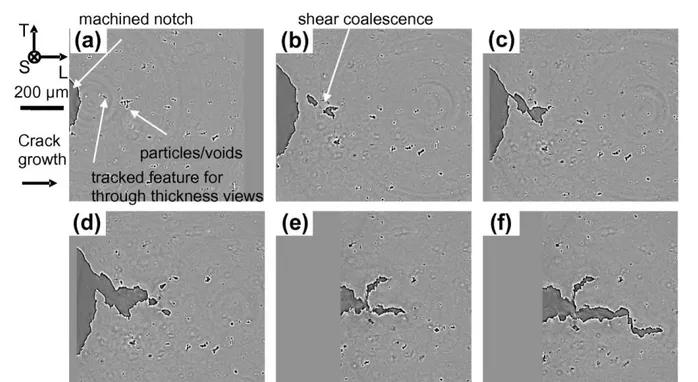
Experimental observations of these micromechanisms are shown in Figure 1. Due to the low particles and voids volume fraction of the material shown in this figure, the influence of the microstructure on the crack propagation path can be observed, but void nucleation micromechanisms cannot be clearly distinguished. A better view of ductile fracture at the microscale is shown in Figure 2. The material shown in this figure has a high nodules volume fraction, which allows to distinguish void nucleation mainly by debonding, with some fragmentation, followed by void growth and coalescence. The initiation and propagation of a macroscopic crack by void sheeting along the shear band can also be observed.

Modeling all these micromechanisms is a computationally challenging problem. Indeed, it raises a number of issues for computational fracture mechanics approaches. While crack modeling techniques that can handle multiple crack initiation sites can be found, it will be shown in this review that there are only a few methods that can also handle large deformations and cracks coalescence. For instance, Antretter and Fischer (1998) have focused on simple two-dimensional (2D) configurations with a single pre-existing crack, and ad- dressed only the influence of particles on crack propagation within the matrix. Simulations with multiple crack initiation sites at arbitrary locations with both particle fragmentation and debonding modeling in 3D can be found in Shakoor et al (2017a). The latter study assumes a brittle fracture of particles and their interfaces, while void growth and coalescence are assumed to be purely plasticity driven.

As pointed out by Teko˘glu et al (2015), recent experimental evidence suggests that for some materials and loading conditions a minor void population nucle- ates, grows, and coalesces within the matrix. This void population is coined as minor due to its small size compared to voids that nucleate due to particles debonding and fragmentation. As explicitly meshing these voids along with particles and voids of the major population would be computationally extremely demanding, Areias et al (2015) among others have relied on continuous approaches. Continuous approaches are computationally interesting as they can represent very large numbers of voids at low computational cost, and with low implementation burden as opposed for instance to remeshing techniques or the eXtended Finite Element Method (X-FEM). However, continuous approaches require to define a so-called Continuous-Discontinuous Transition (CDT), at which the minor void population

(4)

Fig. 1 Cross section from 3D X-ray images of the microstructure of a thick notched specimen under tensile loading at different crack mouth opening displacements: (a) 0 mm, (b) 1.625 mm, (c) 1.875 mm, (d) 2.0625 mm, (e) 2.3125 mm, (f) 2.375 mm. The material, an aluminum alloy with less than 1% initial particles/voids volume fraction, fails by the initiation and propagation of a macroscopic crack in a zig-zag pattern due to the influence of the microstructure. Reprinted from Morgeneyer et al (2011), with permission from Elsevier.

F

thickness

F

250 µm

y

x undeformed state (0) deformed state (7) deformed state (11)

Fig. 2 Cross section from 3D X-ray images of the microstructure of a flat specimen with two machined holes at 45◦ under

tensile loading. The material, nodular cast iron, fails by debonding and fragmentation of the nodules, and then void growth, coalescence and sheeting in the shear band between the two machined holes. Reprinted from Shakoor et al (2017c), with permission from Elsevier.

has grown and coalesced enough so that its size and influence becomes comparable to that of the major void population. At this critical point, one has to consider 3D crack initiation and propagation criteria within the matrix, for instance using the method proposed by Feld- Payet et al (2015).

To follow the emergence of these sophisticated numerical methods, the present review starts in Section 2 by a discussion of numerical methods with a discontinuous modeling of fracture. Here discontinuous implies

that the crack is explicitly modeled, with a discontinuous jump of the displacement field across crack faces. These methods have been developed mainly for brittle materials. They can be applied to model the fracture of brittle components of the microstructures of ductile materials, and also the fracture of ductile components if the softening effect due to the minor void population can be neglected.

Then, methods that can model the softening response of ductile materials are reviewed in Section 3. A focus is made on the application of these methods to the

(5)

matrix component of these materials’ microstructures to account for minor void populations. Additionally, multiscale methods can be seen as continuous methods where the effect of micro-cracks and microstructural damage is modeled using continuous analytic or computational homogenization. This is of particular interest as ductile fracture has to be modeled simultaneously at two or more scales.

Finally, the limitation of continuous methods during the final stage of ductile fracture, where the softening effect becomes predominant over the hardening effect, up to final failure, lead to the CDT problem. This problem can be modeled by coupling continuous models to discontinuous approaches. As detailed in Section 4, this coupling raises other issues that make 3D problems still challenging.

Discussions throughout the paper and in Section 5 should give the reader insights on current and future efforts on micromechanical modeling of ductile fracture. In particular, the authors wish to highlight methods that seem to be the most promising options to handle all difficulties raised by ductile fracture modeling in heterogeneous structures.

2 Discontinuous approaches

If the softening effect before crack initiation and propagation can be neglected, ductile fracture can be modeled using the same numerical methods as brittle fracture. Some differences arise regarding the crack initiation and propagation criteria, as plastic strain and loading path should be accounted for in the ductile case. As this review article does not focus on the criteria but the crack modeling methods, we discard discussions on the criteria. It must however be pointed out that crack propagation criteria are rare for the 3D case, in particular if there are multiple initiation sites as in void nucleation in ductile microstructures. Void nucleation itself is a challenging application for discontinuous approaches, as at the microscale void nucleation can be considered as the brittle failure of particles or particles/matrix interfaces. The main challenge in that case is that these micro-cracks open to a quite large extent before propagating, which restricts the applicability of brittle fracture modeling methods that cannot handle large deformations.

2.1 Element erosion

A simple way to dynamically introduce discontinuities in a FE simulation is to remove elements from the FE mesh and/or the associated contributions from the FE

formulation based on an appropriate fracture indicator. This method is often referred to as element deletion, element removal or kill element. The terms element erosion are used to depict the fact that elements are gener- ally removed after eroding their load carrying capacity over several load increments to avoid convergence issues (Wulf et al (1996)).

When it comes to ductile fracture, the element erosion method is most often associated to Continuum Damage Models (CDMs, see Subsection 3.1). However, some studies can be found where a failure criterion was used to trigger element deletion or erosion without accounting for the softening effect.

Wulf et al (1996) presented an application of element erosion to a 2D aluminum alloy microstructure. Matrix failure was modeled by progressively setting the stress and stiffness of matrix elements to zero depending on a plastic strain based failure criterion. As pointed out by Wulf et al (1996), a strain based criterion is convenient as it also removes distorted elements that should otherwise be treated with mesh adaption (Sub- sections 2.4 and 4.4). Another important remark of the authors is that nodes surrounded with eliminated elements must also be eliminated to avoid the discretization of balance equations to be ill-defined.

A plastic strain based criterion was also used by McHugh and Connolly (2003) to trigger a progressive release of stress and stiffness in given elements. It is important to point out that while the progressive re- laxation is justified as a numerical technique used to improve convergence by Wulf et al (1996), it is defined as a gradual process comparable to the mechanical process of ductile failure by McHugh and Connolly (2003). Thus, the number of load increments over which element erosion occurs is defined as a material parameter by McHugh and Connolly (2003). The proposed application is the microstructure of a metal alloy, wherein the matrix is modeled using a crystal plasticity FE method coupled to element erosion.

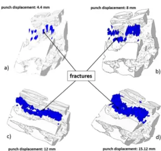
A more advanced empirical criterion accounting for plastic strain and also the stress state was applied to a dual phase steel by Perzyn´ski et al (2017). In particular, 2D and 3D micromechanical simulations accounting for ductile fracture of the ferrite phase were conducted. The ductile fracture indicator was fitted to experimental data giving the plastic strain at failure for ferrite at different stress triaxiality ratios. As shown in Figure 3, promising simulation results of the failure process of dual phase steel microstructures were obtained. These results showed the interaction between brittle fracture in the martensite phase, and ductile failure in the fer-

(6)

rite phase.

Fig. 3 Micromechanical simulation of a 3D dual phase steel microstructure showing in white the martensite phase, and in blue eroded elements from the ductile ferrite phase. The reader is referred to Perzyn´ski et al (2017) for indications on the relation between punch displacement and boundary conditions at the microscale. Reprinted from Perzyn´ski et al (2017), with permission from Elsevier.

In spite of these interesting applications, element erosion has well-known mass loss, mesh size dependence and element shape dependence issues (Mediavilla et al (2006a)). Computational approaches to ductile fracture at the microscale decades ago (Wulf et al (1996)), at a time where high performance computing capabilities were not as accessible as today, used this method. This is mainly due to its ease of implementation and low computational cost compared to the methods that are discussed in the following. The aim of these methods is to allow the modeling of cracks as new interfaces inserted dynamically during the FE simulation. To avoid the numerical issues raised by the element erosion method, the following methods are designed so that cracks can be initiated at arbitrary locations and propagated along arbitrary directions, independently of the FE mesh. 2.2 Enriched Finite Element methods

2.2.1 Introduction

In order to model discontinuities without element erosion or remeshing, a family of enriched FE methods have been developed and have been documented by different authors (Jir´asek (2000); Oliver et al (2006);

Fries and Belytschko (2010)). The most popular of these methods is the X-FEM (Mo¨es et al (1999)), which is based on the partition of unity concept (Babuska and Melenk (1995)). The Generalized Finite Element Method (GFEM) is another relevant enriched method (Strouboulis et al (2000)). Initially, in GFEM, all the nodes in the discretization were enriched; later, local enrichment was adopted. The distinction between X-FEM and GFEM has become less clear as the methods have evolved (Fries and Belytschko (2010)). A very attractive feature of these methods is the fact that discontinuities might be modeled independently of the mesh, i.e., conformity is not required. Most of the applications of enriched FE methods have been dedicated to brittle fracture. This subsection discusses some of the works that have dealt with ductile fracture.

2.2.2 Strong discontinuities

Strong discontinuities such as cracks and holes can be modeled with enriched FE methods. The material/void interface is captured thanks to a discontinuous enrichment, typically using the Heaviside function as enrichment function (Mo¨es et al (1999)). To capture the stress singularity in the near crack tip region, an additional enrichment is necessary (Belytschko and Black (1999)). The latter requires careful choice of the enrichment function, and knowledge of the analytic solution. These enrichment techniques are usually implemented locally and not in the whole FE mesh. This constitutes the basis of X-FEM.

Sukumar and Belytschko (2000) showed how the basic methodology can be extended to account for arbitrary branched and intersecting cracks in 2D cases such as a cross or star shaped crack. An extension to 3D of the basic X-FEM methodology was provided by Sukumar et al (2000) by enriching the elements near the crack front with the radial and angular behavior of the 2D asymptotic crack tip displacement field. Anal- ogous development have been made with the GFEM (Duarte et al (2001)). Further flexibility in the descrip- tion of the crack geometry was introduced by coupling the Level-Set (LS) method (Osher and Sethian (1988)) to the X-FEM: the zero isovalue of a signed distance function gives the position of the crack surface, and its intersection with a second and almost orthogonal signed distance function describes the crack front (Mo¨es et al (2002); Gravouil et al (2002)). The semicircular crack in a Maltese cross modelled by Mo¨es et al (2002), is an example of the more complex and non planar crack geometries that can be studied with this technique.

(7)

2.2.3 Weak discontinuities

When the X-FEM is used to model a strong discontinuity, the crack is embedded within some FE elements, that will distort significantly due to the displacement jump. The X-FEM can also be used to define a stress/strain jump with a continuous displacement. This is relevant for the modelling of inclusions in ductile fracture simulations.

Sukumar et al (2001) presented 2D examples of inclusions to show the potential of this approach to represent complex internal boundaries. In the elements con- taining the matrix/inclusion interface, i.e., the weak discontinuity, the absolute value of an LS function was used as enrichment function. This aspect was further explored by Huynh and Belytschko (2009) with 2D and 3D examples in composite materials. More sophisticated approaches for modeling inclusions with the X- FEM have been developed more recently. Wang et al (2016) proposed an adaptive X-FEM strategy coupling the X-FEM to mesh adaption techniques (Subsection 4.4), and compared its accuracy and computational performance with standard X-FEM.

Some works have applied the capabilities of X-FEM to modelling weak discontinuities along with cracks in ductile materials. Singh et al (2011) studied the effect of the presence of minor cracks, voids and inclusions in the vicinity of a major crack for multiple configurations. Ye et al (2012) analyzed the stress dissipating effect under small strain of reinforcing particles on fatigue close to the crack tip. Metal matrix composites of various particle sizes were investigated. A multiscale approach with the projection method (Loehnert and Belytschko (2007)) was used by Liu et al (2017a) to assess the effect of micro-cracks, inclusions and voids for different rela- tive positions with respect to the tip of a major crack under mode I and mode II loading. These three cited works investigated only 2D configurations.

2.2.4 Discussions

Enriched FE methods provide the capability of mod- elling weak and strong discontinuities, i.e., interfaces between two material phases (Sukumar et al (2001); Huynh and Belytschko (2009)) and void/material interfaces (Mo¨es et al (1999)), as well as stress singu- larities (Belytschko and Black (1999)). These methods can handle branching and intersecting cracks (Suku- mar and Belytschko (2000); Belytschko et al (2001)), non planar cracks (Mo¨es et al (2002); Gravouil et al (2002)) and complex 2D and 3D geometries (Sukumar et al (2000)). These features are relevant for the study of ductile damage.

Yet, most of the literature is dedicated to brittle fracture. Even in works in which ductile materials are the object of study (Loehnert and Belytschko (2007); Liu et al (2017a)), the focus is on the calculation of stress intensity factors and large deformations are not pursued. The small number of works with enriched FE methods dedicated to ductile fracture might be par- tially explained by the fact that these methods were conceived precisely to avoid remeshing, which might be necessary if the considerable deformation associated to ductile fracture is to be accounted for, even with an enriched FE formulation.

The practical application of enriched FE formulations is less straightforward than the implementation of its basic techniques; limitations and additional compli- cations arise. Their implementation can be burdensome depending on the structure of the FE code due to the variable number of degrees of freedom that comes with local enrichment (Rabczuk et al (2010)).

Traditional Gauss quadrature is not adequate for enriched elements. There are different strategies to tackle this problem, but the most common one is subpartion- ing of enriched elements, with higher order integration for crack tip elements (Mo¨es et al (1999)).

In the first X-FEM implementations, topological en- richment was used for the crack tip enrichment, i.e., only those nodes whose support contained the crack tip were enriched. This resulted in a deteriorated order of convergence. To solve this issue, a geometric enrichment was proposed where enrichment is added for all nodes within a distance to the crack tip (Laborde et al (2005)). Although this improves the convergence rate, the conditioning is deteriorated and the problem size increases (Sukumar et al (2015)). Another factor that might affect the order of convergence is the use of ap- proximate enrichment for the crack tip instead of full enrichment (Huynh and Belytschko (2009)).

Ill-conditioning can also arise if an element is cut by an interface such that one of the resulting subvolumes is comparatively very small with respect to the other. To alleviate the conditioning problems associated to X- FEM, ad hoc preconditioners have been proposed, an example of which can be found in B´echet et al (2005). X-FEM related convergence issues are, however, lesser than those that have been found for mixture laws and multiphase elements (Wulf et al (1996)).

An additional obstacle to the application of enriched FE methods to ductile fracture problems is related to their application beyond elastic problems. Even though bimaterial interfaces or void/material interfaces can be handled transparently independently of the behavior of the material, crack tip enrichment functions depend on

(8)

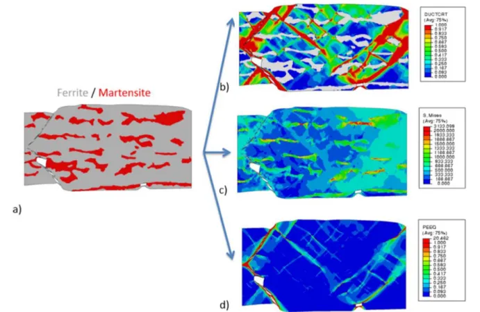
material behavior. Although some developments have been made for elasto-plastic materials (Elguedj et al (2006)), their application remains restricted to confined plasticity, and enriching crack tip elements for more advanced material laws remains a considerable challenge. These drawbacks of X-FEM might deter from its application to ductile fracture problems. Indeed, the number of works that employ it to study ductile fracture is very small with respect to brittle fracture. It should nevertheless not be discarded as it can be applied to model the fracture of brittle components in ductile materials’ microstructures. For instance, the failure of ductile dual phase steels has been studied at the microscale by applying the X-FEM to the brittle marten- sitic phase (Vajragupta et al (2012); Ramazani et al (2013); Perzyn´ski et al (2017)). As shown in Figure 4, remarkable results can be obtained using this approach. However, due to technical limitations, Perzyn´ski et al (2017) used two separate codes for brittle and ductile failure, and enriched elements were considered as deleted in the ductile fracture code.

Void nucleation by fracture of brittle components within ductile materials’ microstructures can hence be modeled using the X-FEM. Enriched FE methods are nevertheless not applicable yet to model the growth of these cracks into large voids.

2.3 Cohesive Zone Models

While enriched FE methods solve completely the mass loss, mesh size dependence, and element shape issues raised by the element erosion method, they fall short in modeling the energy dissipation rate. Indeed, once a displacement jump is introduced within an element, its load carrying capacity is instantly lost. In element erosion, the energy dissipation rate could be controlled based on numerical (Wulf et al (1996)) or physical ar- guments (McHugh and Connolly (2003)) by progressively setting the stress and stiffness to zero. When the crack is defined not by element removal but by an actual interface across which the displacement is defined as discontinuous, Cohesive Zone Models (CZMs) can be introduced to model the energy dissipation rate.

The origins of CZMs date back to the 60’s and the concepts were initially introduced by Barenblatt (1962) and latter described by Rice (1968a). The concept of CZM is simple and states that, at the crack tip, there is a finite size region where the material transitions from a fully broken material to a sound material. Figure 5 shows a schematic representation of a fracturing process taking place on a brittle material and its interpre- tation using a CZM model. This region, called the cohe-

sive region or process zone, corresponds to prospective fracture surfaces ahead of a crack which are permitted to separate under loading. This separation process and crack surface creation process are opposed by atomic or molecular cohesive forces (Rice (1968b)). The energy dissipated by the breakage of the atomic bounds corresponds to the fracture energy required to create the new free surfaces and break the material.

The force opposed to the opening of the new surfaces is called cohesive force and modeled by a phe- nomenological traction-separation law. There are many traction-separation laws that can be used to model the fracture process.

In comparison with other methods used to model fracture, cohesive elements are independent from mechanical behavior of the bulk material, the extend of the cracks and the size of the plastic zone (Ortiz and Pandolfi (1999)), which represents a very interesting advantage. Within the context of FE models, there are different ways of using CZMs. Enrichment based numerical techniques, such as XFEM or GFEM (Mo¨es et al (1999); Strouboulis et al (2000); Reed and Hill (1973); Arag´on and Simone (2017)), will not be discussed in this subsection. These techniques are used by a large part of the community, in particular XFEM approaches which are discussed in Subsection 2.2. An- other technique is based in the insertion of “cohesive elements” into the mesh. These cohesive elements, which can be seen as some kind of special surface element, obey a constitutive law that corresponds to the selected traction-separation law.

In practical terms, a cohesive element is inserted at a face separating two bulk elements as it can be seen in Figure 6A. The insertion is simply performed by duplicating the nodes forming the separating face and insert- ing a new cohesive element linking the original nodes to the new duplicated ones (Figure 6C). It is worth men- tioning that cohesive elements are initially flat (Figure 6B) and, in contrast to a regular bulk FE, this flatness does not represent any issue regarding the capability of cohesive elements to properly describe the mechanical response of the process zone.

The implementation of CZMs into a FE framework has strong implications on the way cohesive elements can be used to model fracture and, in some cases, can represent a limitation of the method. Some of these limitations are presented here and classified by different topics: insertion methods and crack propagation approaches.

(9)

Fig. 4 Micromechanical simulation of a 2D dual phase steel microstructure showing the ductile fracture of the ferrite phase modeled using element deletion and the brittle failure of the martensite phase modeled using X-FEM. (a) Microstructure with ferrite in gray and martensite in red. (b) Damage variable in ferrite phase. (c) Von Mises stress field. (d) Equivalent plastic strain field. Reprinted from Perzyn´ski et al (2017), with permission from Elsevier.

2.3.1 Insertion methods

Intrinsic methods The simplest way of handling cohe- sive element insertion is to insert these elements since the beginning of the simulation. This approach is very interesting since its implementation in any standard FE code is straightforward and many problems such as particle debonding can be simulated with this approach. However there is a strong drawback: an artificial re- duction of the stiffness of the material is induced. In fact, most traction-separation laws have an initial region where the traction increases monotonically from a zero up to a maximum value (in some cases this increase is linear). This increase of the traction level as a function of the opening displacement leads to the introduction of an artificial stiffness into the system that mod- ifies the macroscopic response of the material (Tomar et al (2004)). A way to overcome this problem is to use an infinite cohesive stiffness up to the critical cohesive traction. This can be achieved by introducing Lagrange multipliers in such a way that the opening of the element is only allowed once a critical traction is achieved (Lorentz (2008)). However this solution re-

quires the modification of the standard FE formulation and, in this way, the main advantage of the approach (the use of a standard FE code) is lost.

Extrinsic methods An alternative method to handle the insertion of cohesive elements is to dynamically dupli- cate the nodes of faces where a given criterion is satisfied and then insert the new cohesive element. This technique is very interesting because it allows to get rid of the artificial modification of the global stiffness of the material but its implementation is not straightforward. The implementation requires the modification of the core features of the FE library, in particular con- cerning the mesh module, and it is particularly complex within the context of distributed computing (Vocialta et al (2017)). Although this extrinsic approach allows to circumvent spurious stiffness problems, it still suffers from some mesh dependency problems, as discussed in the following.

2.3.2 Crack propagation approaches

Mesh dependency Whether an intrinsic or an extrinsic approach is used, CZMs within the context of FE meth-

(10)

Fig. 5 Schematic representation of the cohesive zone: transition from sound material to broken material. The green ar- rows represent the distribution of tractions over the cohesive region.

Fig. 6 Schematic representation of the insertion of a cohesive element: A. The green dashed line shows the faces that will be split. B. The cyan dots correspond to the nodes that have been doubled and therefore there are indeed two nodes at the same location. The green line corresponds to a initially flat cohesive element. C. After loading the new inserted cohesive elements open.

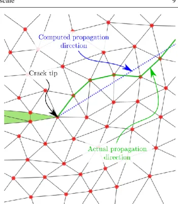
ods suffer from mesh dependency. In fact since cracks appear at the faces separating two bulk elements, therefore the crack path depends on the mesh and this is true for simulations involving structured and non structured meshes. The issue is illustrated in Figure 7 where the predicted crack path and the actual one are shown in blue and green, respectively. This means that if the mesh changes, the crack pattern slightly changes too.

Fig. 7 Prescribed crack path (dashed blue line) and the actual crack path (solid green line) after cohesive elements insertion.

Debonding It is therefore clear that the CZM is very well adapted for problems where the crack path is known in advance. This is the case of problems involving debonding of interface. The literature studying the application of CZM to this kind problems is rather broad (Chandra et al (2002); Turon et al (2007); Li and Ghosh (2004); Turon et al (2010)). In the case of microscopic modeling of materials, the CZM are very well suited to model the debonding that can take place between the inclusions and the matrix of a metallic or composite material. 2.3.3 General remarks

CZM within the context of FEs represent a very interesting tool regarding fracture modeling. The discontinuities of displacement fields that appear during the fracture process are naturally handled by the method. It also allows to introduce interesting physical mechanisms into the fracture model through the use of different kind of traction-separation laws and the energy dissipation rate can be controlled very accurately. These traction-separation laws can include rate effects (Salih et al (2016)), account for stress triaxiality ratio (Baner- jee and Manivasagam (2009)) and fatigue effects (Nguyen et al (2001)), among others.

Cohesive elements are widely used in the community for applications involving brittle materials and also within the context of fragmentation where most materials fail in a brittle fashion under violent dynamic load-

(11)

ings. Although some traction-separation laws for ductile materials exist (Scheider (2009)), problems arise when ductile materials are subjected to complex non propor- tional loadings and, in particular, to low stress triaxiality ratio loading. These problems come from the fact that it is still a big challenge to handle contact in problems involving non monotonic loading path that can eventually lead to crack closure and friction.

There are also some drawbacks that often restrict the use of CZM in classical FE codes. The need of handling mesh operations to dynamically insert cohesive elements (extrinsic approach) is extremely important and mesh dependency remains an issue regardless of the insertion approach. Recent approaches as the one introduced by Soghrati et al (2017) tackle mesh dependency issues. Alternatively, mesh dependency issues related to CZMs can be overcome by using advanced crack initiation and propagation techniques (Subsections 2.2 and 2.4).

In spite of the drawbacks discussed previously, CZMs present interesting features that can be used within the context of heterogeneous materials modeling. A brief overview of different works using CZMs to study heterogeneous materials is proposed in the following. 2.3.4 Applications to heterogeneous materials It is now clear that cohesive elements can be used to study the fracture of heterogeneous materials but it is necessary to use this technique carefully since its drawbacks could lead to non physical results. Taking into account the advantages and drawbacks of CZM presented previously, CZMs have mainly been used for problems involving debonding between inclusions and the matrix (Liang and Sofronis (2003); Meng and Wang (2015); Giang et al (2017)), inclusions failure (Steglich et al (1999); Giang et al (2017)), and problems where the crack paths are prescribed (Giang et al (2017)). The previous cited works will be briefly discussed.

Steglich et al (1999) proposed an interesting and pi- oneering application of cohesive elements to the modeling of fracture of metal matrix composite materials for which failure is dominated by particle cracking. At the macroscopic level, the damage process for this material was modeled using a Gurson-Tvergaard-Needleman (GTN) model (Section 3). The parameters of this mi- cromechanical CDM model were obtained from unit cell computations where the two phases of the material (inclusions and matrix) were meshed. Cohesive elements were initially placed over the equatorial plane of the inclusion and the failure process was modeled by using a classic exponential traction-separation law (Xu and

Needleman (1994)). Although inclusion/matrix debonding and matrix failure was neglected in the unit cell computations, the multiscale principle of fitting macro- scopic failure models from simulations of more advanced mesoscopic models was highlighted. A similar unit cell approach modeling the debonding of particles instead of their fragmentation was proposed by Meng and Wang (2015) among others.

Since debonding can be modeled very accurately by using cohesive element approaches, this technique has been widely used within the context of heterogeneous materials. Liang and Sofronis (2003) tackled a very challenging problem that remains a hot topic in the field of metallic materials modeling: hydrogen em- brittlement. It is well know that hydrogen induces em- brittlement of ductile materials as hydrogen induces debonding at the interface between carbides and the matrix. This debonding was modeled by using a traction- separation law that accounts for the hydrogen concentration in the material. Although the use of cohesive elements to study debonding is logic and simple, the coupling of fracture processes with complex multiphysics phenomena is not. It is indeed very interesting to see how complex multiphysics phenomena, such as hydrogen diffusion, can be coupled to the mechanical response of a material containing cracks.

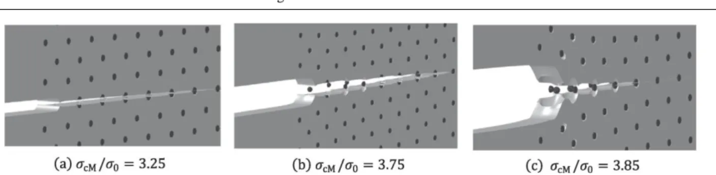
An interesting contribution to micromechanical modeling using CZMs was proposed recently by Giang et al (2017). Ductile fracture was modeled at the scale of large 3D periodic arrays of inclusions. Cohesive elements with a classic exponential traction-separation law (Xu and Needleman (1994)) were placed at interfaces between particles and matrix, and along a predefined crack propagation path. The latter was mainly used to model matrix micro-cracking, but it also included the equatorial planes of some particles, which enabled to model their fragmentation. This is hence a combina- tion of previous works by Steglich et al (1999); Meng and Wang (2015), with the addition of a matrix micro- cracking model. Examples of results using this approach are shown in Figure 8. These results reveal a compe- tition between particle debonding and fragmentation depending on material properties. Although these results are promising, Giang et al (2017) used an intrinsic method and had to define the crack path a priori both for particle fragmentation and matrix micro-cracking. 2.3.5 Conclusion

CZMs are relevant for modeling the initiation and propagation of brittle and ductile cracks. This is done ei- ther by inserting cohesive elements along any potential crack initiation and propagation surfaces, or by dynam-

(12)

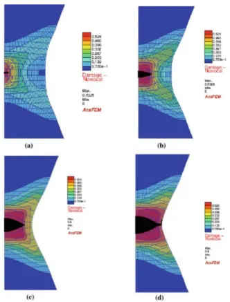
Fig. 8 FE simulation of a ferritic steel microstructure using CZMs at particles/matrix interfaces, and along a predefined crack propagation path through particles and matrix at the midsection of the specimen. The ratio σcM /σ0 is the ratio between matrix

cohesive strength and matrix yield stress. Reprinted from Giang et al (2017), with permission from Elsevier.

ically inserting cohesive elements during the simulation. These elements have a negligible volume initially, and will progressively open as the crack grows, with an ac- curate modeling of the energy dissipation rate through a traction-separation law.

The implementation of CZMs for particle debonding modeling is facilitated, as cohesive elements can be inserted initially or dynamically along particles/matrix interfaces. Particle fragmentation and matrix micro- cracking modeling is less straightforward, as the crack propagation path is generally not known a priori. For such arbitrary crack paths, CZMs should be coupled to the methods presented in Subsections 2.2 and 2.4. For instance, Wolf et al (2017) coupled a CZM to the X-FEM in order to model ductile fracture in 2D configurations.

2.4 Mesh modification 2.4.1 Introduction

CZMs can already be seen as a mesh modification, as new elements are inserted to model the discontinuity. If no CZM is considered, the nodes along the crack path can be simply duplicated. As in element erosion approaches, this instantaneous fracture modeling can be smoothed by releasing node tractions progressively over several increments. It must be pointed out that these smoothing techniques are usually expressed as functions of increments or time, while a CZM is expressed as a function of crack opening displacement (Antretter and Fischer (1998); McHugh and Connolly (2003); Ortiz and Pandolfi (1999)). Cohesive elements also use a surface discretization, while traction release is expressed directly at nodes (Antretter and Fischer (1998)).

Antretter and Fischer (1998) considered a 2D problem of a ductile material with two inclusions explicitly meshed. Crack initiation was not modeled as one of the two inclusions was considered as initially fragmented. The propagation of this fragmentation crack within the

matrix and towards the second inclusion was modeled by triggering node release along a predefined crack path based on a crack tip opening angle criterion.

For arbitrary crack paths where the crack propagation criterion not only determines the propagation on- set, but also the propagation direction, the numerical implementation becomes quite complex. Robust mesh modification operations have to be developed to dynamically discretize new interfaces during the FE simulation, as discussed hereafter.

Note that the terms mesh modification are rarely used. Most authors use the word remeshing, which is a quite ambiguous term as it may encompass full remeshing, local remeshing, or adaptive mesh refinement. The most widely used remeshing technique for large deformations simulations involves a human operator whose role is to correct the initial FE model if element inversion occurs during the simulation. There are automatic procedures to avoid human intervention, although they are often restricted to tetrahedral elements. Automatic remeshing can simply mean moving some nodes to avoid element inversion. This can be combined or replaced by automatic mesh topology changes (e.g., by edge or face swapping). Alternatively, remeshing can mean regenerating the whole mesh from some representation of the current geometry whenever there is a risk of element inversion.

Adaptive mesh refinement, or local mesh refinement, is often presented as a type of remeshing technique, although it only consists in splitting edges, faces, and elements to refine the mesh. Mesh adaption seems to be less ambiguous as it usually means that mesh size is being varied spatially and sometimes also in time to automatically adapt the FE mesh to the solution’s variations. This can be done dynamically and automatically throughout the FE simulation, which requires proper transfer operators to map variables between old mesh and new mesh after the FE mesh has been modified. It can also be done after the whole FE simulation has been conducted, to restart with a new mesh.

(13)

To summarize, we will use the word remeshing whenever a mesh modification is operated to avoid element inversion or modify the model geometry. This modification can be a change to the positions of some or all nodes, and/or a change to the topology of some or all FEs. Full remeshing will mean that the whole FE mesh is being regenerated from some representation of the domain geometry, and in particular of its boundaries (including the crack geometry).

Mesh adaption will refer to mesh modifications operated to adapt the FE mesh to the FE solution’s variations and reduce some estimated error. This may be done solely using local mesh refinement, or accompa- nied by node position and element topology changes.

In all cases, we only refer in the following to automatic mesh modifications that do not require human intervention and can be applied dynamically during the FE simulation, as the crack path is not known a priori. 2.4.2 Methods and their applications

Mediavilla et al (2006a) used an uncoupled non local integral damage indicator as crack initiation and propagation criterion 2_{. This criterion was used to intro-}

duce a new crack geometry, which was itself used as in- put to a full remeshing algorithm. A similar approach was proposed earlier by Bouchard et al (2000), using a stress based crack initiation and propagation criterion. At each load increment, the crack was advanced by a given length, which was considered a purely numerical parameter. The numerical approach proposed by Me- diavilla et al (2006a) consisted in first introducing the new crack segment in the FE mesh, without opening it. Then, an appropriate transfer operator was applied for history variables, before duplicating the nodes along the new crack segment and recomputing strain and stress fields for the new geometry.

While the full remeshing based crack modeling and history variables transfer process used by Mediavilla et al (2006a) may seem quite complex, each step is necessary to ensure consistent mechanical equilibrium throughout crack propagation. Transfer operators are very strongly related to remeshing algorithms, as all mesh modifications, except hierarchical mesh refinement, lead to artificial energy diffusion (Mediavilla et al (2006a); Shakoor et al (2015)). For ductile fracture problems a robust transfer operator to conserve plasticity history variables is of high interest, in particular if the crack

2

The word uncoupled means that in this work the softening effect was not modeled, as opposed to coupled damage models discussed in Subsection 3.1. A non local regularization was

propagation criterion depends on plastic strain (Medi- avilla et al (2006a); Shakoor et al (2015)). A simple solution is to solve mechanical balance equations after each crack initiation or modeling step (Mediavilla et al (2006a); Shakoor et al (2015, 2017a)). An important remark of Shakoor et al (2017a) is that, although a weak (or explicit) coupling between crack modeling and mechanical solution was used, crack initiation and propagation was modeled before mechanical solution. This is a relevant choice for micromechanical analy- sis using computational homogenization, as it ensures that all quantities of interest are consistent with the geometry. To further improve energy conservation during remeshing, higher order interpolation techniques are interesting as they reduce the diffusion induced by the interpolation step between old mesh and adapted mesh (Mediavilla et al (2006a)).

Both artificial energy diffusion and the accuracy of the crack propagation criterion can be improved using mesh adaption. A first a priori error minimization ap- proach is to refine the mesh close to crack faces and especially crack tips (Bouchard et al (2000); Mediav- illa et al (2006a)). More mathematically sound a priori and a posteriori error estimators based on the repre-

sentation of the geometry 3_{have been proposed in the}

literature. In particular, for a first order FE scheme, the geometric error can be expressed as a function of the principal curvatures of geometric boundaries, which can be estimated using distance functions and their second derivatives (Roux et al (2013); Shakoor et al (2015)). Since at least one of the principal curvatures is infinite at crack tips, a minimum mesh size parameter is usually defined to limit mesh refinement in crack tips regions, while mesh size varies smoothly depending on the local principal curvatures in the whole FE domain (Roux et al (2014)). Because principal curvatures are generally different in distinct directions (similarly to principal stresses), anisotropic elements can be used to refine the mesh only in given directions (Roux et al (2013)). These elements are however not recommended for large deformation simulations as they raise a higher risk of element inversion (Shakoor et al (2017b,a)).

Both remeshing and mesh adaption were used for micromechanical ductile fracture modeling by Roux et al (2014), although the proposed approach can be seen as an element deletion, or region deletion method. It consisted in using an LS function and error estimator based anisotropic mesh adaption method to define the crack geometry. Then, instead of introducing a new crack sur-

nevertheless judged necessary by Mediavilla et al (2006a) to ”reduce the influence of local damage variations which are a result of the discretization”.

3

Error estimators can also be based on mechanical variables as discussed in Paragraph 4.4.1.

(14)

face, a region of small thickness was introduced and modeled with a very low stiffness to simulate an actual void. The proposed method enabled void nucleation, growth and coalescence simulations of 2D microstructures of complex morphology, which required a robust remeshing technique to handle very large deformations (Roux et al (2013)). Stress based criteria were used to predict particle fragmentation and debonding.

A limitation of the method proposed by Roux et al (2014) was that the interface between the void region and the other material components (matrix and inclusions) was not meshed explicitly. Thus, material interfaces could cross arbitrarily through some mesh elements, whose behavior was defined using mixture laws. Although these laws can be relevant for multiphase fluid flow modeling (see e.g., Hirt and Nichols (1981)), they cannot define the mixture of an elastic inclusion with an elasto-plastic matrix. An extension to this region deletion method was proposed by Shakoor et al

(2015). To avoid mixture laws4_{, remeshing operations}

were extended to dynamically construct an explicit interface discretization. This method was first applied to model void coalescence by matrix micro-cracking in 2D using an uncoupled Lemaitre damage indicator by Shakoor et al (2015), and later extended to model particle fragmentation and debonding in 3D by Shakoor et al (2017b) for academic test cases.

This region deletion method avoided the mesh shape dependence issue of the element deletion method, as LS functions were used to define any arbitrary shape for the region to be deleted. LS functions are signed distance functions to the interface computed at FE mesh nodes, with an arbitrary sign convention that distin- guishes mesh nodes inside a given component of the material from outer nodes (Osher and Sethian (1988)). For LS functions to be well-defined, the mesh had to be fine enough (or the region thickness large enough) so that some nodes would be located within the region to be deleted (and thus have a different sign from other nodes of the FE mesh). Although in ductile fracture cracks grow up to become large interacting voids, this requirement on mesh size raised computational cost issues (Roux et al (2014)), even if interfaces were explicitly meshed (Shakoor et al (2015, 2017b)). This limitation was removed by Shakoor et al (2017a), where the authors proposed to use multiple LS functions to capture the crack geometry, as proposed by Sukumar et al (2001) in the context of the X-FEM. Two LS functions were used to define the two faces of the deleted region (the two crack faces), while a third LS function was used to delimit its extent (the crack tip). The thickness

4

Element enrichment approaches such as the X-FEM can also be used (Subsection 2.2).

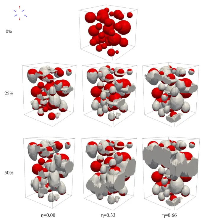
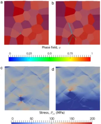
of the deleted region could then be reduced to at least one order below mesh size. This framework was applied to model crack initiation in 3D using stress based particle fragmentation and debonding criteria by Shakoor et al (2017a). As shown in Figure 9, this framework is promising as the large deformation of nucleated voids can be tracked up to the void coalescence phase. Re- sults at 50% of applied strain in Figure 9 illustrate well these capabilities provided by remeshing methods. 2.4.3 Discussions

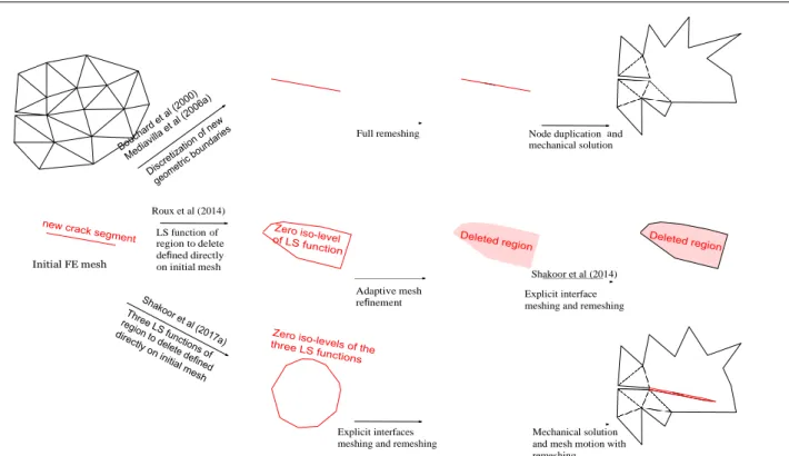
Remeshing and mesh adaption based crack modeling methods are summarized in Figure 10. An advantage of the methods proposed by Roux et al (2014); Shakoor et al (2015, 2017a) over those proposed by Bouchard et al (2000); Mediavilla et al (2006a), is that they used a local mesh modification algorithm (Gruau and Coupez (2005); Shakoor et al (2017b)), instead of regenerating the whole mesh at each initiation or propagation step (i.e., full remeshing). This is relevant for:

– conservation of history variables, because numerical

diffusion is only introduced close to the crack tip, where the mesh is finer,

– computational cost, as mesh modification operations

are restricted to a small region,

– distributed computing, as independent and spatially

local operations are easier to distribute among multiple processors.

It can be observed in Figure 10 that the methods developed by Shakoor et al (2015, 2017a) place FEs within the crack or deleted region. Since crack faces are explicitly meshed in these methods, one could consider removing these elements. However, the mesh motion and adaption method proposed by Shakoor et al (2017b) uses these elements within the crack or void to model its growth and linkage with neighboring voids.

The main limitation of remeshing and mesh adaption based crack modeling is the high technicality of mesh modification operations and the difficulty to im- plement them, especially in 3D, in comparison to element erosion for instance. Additionally, the difficulty is severely increased if the mesh comprises elements of different types and higher order. Mediavilla et al (2006a) developed an algorithm for quadrangle elements in the 2D case, but linear tetrahedra are systematically used in 3D to avoid the difficulty in adapting meshes with hexahedral or higher order elements. Shakoor et al (2017a) alleviated the difficulty of updating crack geometry by using LS functions, but no 3D crack propagation criterion was proposed. Crack propagation techniques introduced earlier by Carter et al (2000) could complete

(15)

Fig. 9 Micromechanical simulations of a metal matrix composite microstructure showing remeshing based modeling of void nucleation by particle debonding and fragmentation followed by void growth and coalescence. Voids are shown in light gray, particles in red, and η refers to the stress triaxiality ratio. Reprinted from Shakoor et al (2017a), with permission from Elsevier.

the method of Shakoor et al (2017a). The latter only focused on void nucleation for a high particle volume fraction metal matrix composite for which matrix micro- cracking was neglected and void coalescence was assumed to be purely plasticity driven.

As a conclusion, discontinuous approaches to ductile fracture where crack initiation and propagation are modeled using mesh modifications have been developed in the two last decades. In particular, these methods

have extensively been applied to model the brittle fracture micromechanisms of particle fragmentation and debonding which play a major role in ductile fracture. The use of remeshing in these developments is justified by a large deformation of crack faces and a significant void growth before final failure. Remarkable results have been obtained regarding crack initiation in 2D and 3D, but crack propagation modeling is for the moment restricted to 2D. This limitation does not seem to be linked to the crack modeling methods, as has already

η=0.66

η=0.33

η=0.00

50%

25%

0%

(16)

Node duplication a mechanical solution Adaptive mesh reﬁnement Shakoor et al (2014) Explicit interface meshing and remeshing

Explicit interfaces meshing and remeshing

Mechanical solution and mesh motion with remeshing

Fig. 10 Summary of remeshing and mesh adaption based discontinuous approaches. In the first line, crack meshing and node splitting as proposed by Bouchard et al (2000); Mediavilla et al (2006a). In the second line, region deletion with an LS function as proposed by Roux et al (2014), possibly with an additional explicit interface meshing step as proposed by Shakoor et al (2015, 2017b). In the third line, crack meshing and node splitting using three LS functions as proposed by Shakoor et al (2017a). Mesh modifications are systematically followed by the transfer of history variables.

been observed in Subsection 2.2, but to the absence of 3D crack propagation criteria that can handle multiple crack initiation sites.

2.5 Conclusion

While they cannot account for the influence of a minor void population within the matrix, the computational methodologies reviewed in this first section already reveal the complexity of ductile fracture modeling at the microscale. The features of interest for discontinuous approaches are mesh independence, energy dissipation rate modeling, compatibility with large deformations, and ease of implementation.

Removing any elements that are too distorted or have satisfied some fracture criterion is the most straightforward discontinuous approach. It is easy to imple- ment, and solves any element inversion issues in large deformations. It can be completed with a progressive release of stress and stiffness tensors to control the energy dissipation rate. However, it raises mesh size and mesh element shape dependence issues as the crack can only propagate from element to element. Removing elements also leads to a loss of mass.

As a consequence, there is a need for methods that can model cracks as new interfaces dynamically and arbitrarily inserted and modified during the FE simulation, depending on some crack initiation and propagation criteria. The first option to reach such end is enriched FE methods, and in particular the X-FEM. This method enables to define interfaces independently of the FE discretization, as cracks can cross mesh elements and crack tips can be embedded within elements. The implementation of the X-FEM requires some modifications to the FE code as additional degrees of freedom are added, and some numerical issues have to be handled. Apart from these difficulties, it seems a perfect candidate to model the failure of brittle components of ductile materials’ microstructures. However, it has been applied mostly to brittle materials. This is due mainly to the impossibility of modifying enriched FEs and thus ensuring these elements keep a good shape throughout the deformation process. There is hence a need for improved versions of these enriched FE methods so that large deformations can be handled.

The second option for initiating and propagating arbitrary cracks without any mesh dependence is through remeshing. The latter can naturally handle large deformations as distorted FEs can be eliminated by topological operations. However, remeshing has some conse-

Full remeshing nd Roux et al (2014) Initial FE mesh LS function of region to delete deﬁned directly on initial mesh

(17)

− quences that require a special care. First, it can induce

unbalance and significant diffusion if a proper transfer operator is not implemented. Second, its implementation is quite complex especially in a distributed computing context, although this difficulty is alleviated if local remeshing is used instead of full remeshing. Re- cent FE simulations of ductile fracture at the microscale show that remeshing based techniques are a promising discontinuous approach. These remarkable simulations show void nucleation by failure of brittle components or their debonding, and the growth of these voids up to large sizes where they start interacting by plastic localization. There is no example of a similar result obtained with enriched FE methods.

Neither the X-FEM nor remeshing based techniques have a built-in model for the energy dissipation rate. The latter can be modeled using CZMs. Indeed, while CZMs alone have limiting mesh dependence issues, developments coupling CZMs to the X-FEM have shown that this limitation can be overcome. There is however no study showing the compatibility of CZMs with remeshing, especially in the large deformations case.

Finally, both enriched FE methods and remeshing based techniques require appropriate crack initiation and propagation criteria. While 3D particle debonding and fragmentation criteria have been mentioned in this section, there is still much work to be done regarding 3D crack propagation. The capabilities of existing 3D crack propagation methods have not been demon- strated for problems with multiple crack initiation sites and large deformations yet. It is a main limitation of discontinuous approaches that can be overcome by using continuous approaches to model crack propagation within the matrix material.

3 Continuous approaches

As stated in Section 2, robust and stable discontinuous approaches have been proposed and applied in the literature to model the brittle failure of particles and their interfaces. The energy dissipation rate can be modeled using CZMs. Mesh independence can be achieved using the X-FEM or remeshing based techniques. The latter have also been proven interesting capabilities in handling large deformations and purely plasticity driven void coalescence within the matrix.

In this section, a more complete model accounting for the nucleation, growth and coalescence of sub- micron sized voids within the matrix material is thought through. While discontinuous approaches could theo- retically be used once again, this would lead to an extremely high computational cost. For instance, O’Keeffe

et al (2015) report that for the studied aluminum al-

loy, a small volume containing on the order of 102

par-

ticles would contain on the order of 107_{minor voids.}

To avoid this prohibitive computational cost, continuous approaches have been considered in the literature. These approaches have initially been proposed to model the influence of the major void population on material behavior at the macroscale. There are herein considered to model the influence of the minor void population on matrix behavior at the microscale.

Continuous approaches consist in modeling the influence of minor voids as a homogenized effect leading to a continuous material degradation process. An advantage of continuous approaches is that damaged regions can naturally grow, branch, coalesce without any numerical difficulty. Full material degradation and the initiation and propagation of cracks within damaged regions require a proper CDT model. CDT modeling, including Phase-Field (PF) models, is not discussed in the present section but in Section 4, as well as applications of continuous approaches beyond the void coalescence phase.

3.1 Continuum Damage Models

CDMs are certainly the most active and widely used modeling approaches to ductile fracture in the recent literature. This is in part due to their implementation in commercial codes, and the ease of implementing new ones as user subroutines. Some of these codes also include regularization techniques, which will be discussed hereafter.

3.1.1 Models

On the one hand, when it comes to fracture problems at room temperature, the Lemaitre model seems to be adopted by most researchers (Vaz and Owen (2001); Andrade Pires et al (2004); C´esar de S´a et al (2006); Bouchard et al (2011); Seabra et al (2013)), for instance to model cold metal forming processes. It can be coupled to the Johnson-Cook elasto-viscoplastic model to address rate dependent problems (Broumand and Khoei (2015)). The Lemaitre model is based on a dam- age variable D and an effective stress definition σeff =

σ _{, first proposed by Kachanov (1958), which cor-}

1 D

rects the conventional stress tensor σ to account for the presence of voids. This definition of σeff requires

D to be comprised between 0 (defect free material) and 1 (fully degraded material). Many authors use empiri- cal evolution laws for D (Borouchaki et al (2005); Me- diavilla et al (2006b); Areias et al (2011)). The work