Abstract— Frequency dynamics studies are important at Hydro-Québec (HQ). Wind integration raises questions about HQ ability to maintain frequency regulation in normal operation and during contingencies. Quasi Steady-State (QSS) approximation is the best alternative to simulate long-term voltage and frequency dynamics without compromising the exactness of simulation results. Collaboration between HQ and University of Liège allowed the development of numerous models. Frequency dynamics is represented by machines inertia, speed governors and a complete AGC controlling 13 hydro power plants including transmission delays. For voltage dynamics, static var compensators, synchronous condensers and tap changer transformers are also represented. Wind farms are modeled as generation patterns (Pwind = f(t))
including a Wind Farm Management System (WFMS). This paper addresses wind farm integration and AGC frequency regulation. Based on HQ field measurements and observations, the most pessimistic cases were simulated. Two scenarios are detailed: the 3500 MW of wind farms currently planned for 2015 and a hypothetical 10 000 MW of wind integration. The results show that actual AGC settings are accurate for the planned wind farms, but might need some changes for a 10 000 MW scenario.
Index Terms--AGC, frequency dynamics, governors, load variations, quasi steady-state time simulation, wind generation patterns.
I. INTRODUCTION
ydro-Québec (HQ) network is about 40 000 MVA during peak load and is asynchronously linked to the north-eastern interconnection. Frequency regulation in normal operation and during contingencies is a big concern due to the relatively small size of the islanded HQ network. Frequency deviation can go up to +/- 1.5 Hz under contingency before SPS action (Under Frequency Load Shedding & Generation dropping) [1].
Wind integration raises questions about HQ ability to maintain frequency regulation [2] [3]. Currently, about 650
S. Lebeau is with Hydro-Québec TransÉnergie, Bulk and Interconnections Network Strategies Department, Complexe Desjardins, CP 10000, Montreal, Canada, H5B 1H7.
N. Qako is with Hydro-Québec IREQ, Power Systems and Mathematics Department, 1800 boul. Lionel-Boulet, Varennes, Canada, J3X 1S1.
T. Van Cutsem is with the Belgian national Fund for Scientific research (FNRS) at the Dept. of Electrical Engineering and Computer Science (Montefiore Institute) of the University of Liège, Sart Tilman B37, B-4000 Liège, Belgium.
MW of wind power plants are in service, expecting 3500 MW for 2015. A call for tenders has been launched for 500 MW of additional small wind farms (under 25 MW). Different studies are in progress to evaluate the maximum wind power that HQ can handle regarding frequency and voltage regulation.
The purpose of this paper is to simulate load ramps and area interchange variations with wind generation changes in order to verify frequency and voltage regulation regarding the Automatic Generator Control (AGC) behavior and settings. Voltage regulation is also briefly discussed.
To have a good approximation of the frequency and voltage regulation, simulation were made on a 30 minute period using Quasi Steady-State approximation (QSS). HQ already uses QSS to study the voltage stability limits of its network. Some Reliability Operating Limit (ROL) of HQ bulk system are determined with those studies. The software is also used for long-term simulation of frequency dynamics, as shown in this paper.
Based on HQ field measurements and observations, the most pessimistic cases were simulated. Simulations take into account the combine effects of:
• Load level (between 15 000 and 40 000 MW)
• Area interchange variations (up to 1500 MW in 10 minutes) • Load following (up to 2500 MW over a 30 minutes period) • Variation of Wind farm generation (up to 25% in 30 minutes).
One of the worst scenarios for HQ is a wind generation decrease with rising load and exports on a low load network. HQ frequency regulation and spinning reserve are mainly done by the hydro plants. Normal operation of hydro generators is at optimal generation which is near maximum opening of the governors gates. This gives a small operating range. The reverse situation is less severe because hydro generators can handle a significant overfrequency. If the wind generation increases, the hydro generation will decrease, leaving more power available to the AGC.
Fig. 1 shows a typical wind power variation (SCADA values). On July 1st 2010, during a 30 minute period, the
total wind power decreased by 20% (from 237 to 107 MW
Wind integration and AGC frequency dynamics
simulations using Quasi Steady-State
approximation
Simon Lebeau Niko Qako Thierry Van Cutsem, Fellow, IEEE
for a 650 MW installed capacity). Combined with 200 MW of rising load and load level at 17 500 MW (less than 50% of peak load), this is the kind of scenario addressed by this paper.
Fig. 1. HQ total wind power generation between 16h15 and 16h45 on July 1st 2010 (SCADA data).
The paper is organized as follow: in section II, the software and models used are described. Simulation results for 3500 and 10 000 MW of wind power integrated to the HQ network are shown in section III. An overview of the future development is discussed in section IV.
II. MODELING
A. Quasi Steady-State Approximation
In order to simulate accurately frequency events, simulations were made over a 30 minute period. Full Time Scale simulation is way too long to be a good solution. QSS approximation is the best alternative to simulate long-term voltage and frequency dynamics without compromising its exactness. Collaboration between HQ and University of Liège allowed the development of numerous models. Frequency dynamics is represented by machines inertia, speed governors [5] and a complete AGC. For voltage dynamics, machines exciters, static var compensators, synchronous condensers and tap changer transformers are also represented [6].
An advantage of QSS simulation is its fast computing time. It takes about 60 seconds of computing time for a 30 minutes simulation at time step of 0.1 seconds.
B. AGC
Since HQ is an islanded network, AGC is use to regulate frequency by dispatching generation to 13 assigned power plants. The HQ AGC is fully represented with all delays and the same signal names used at the Electricity Management System (EMS).
The first part of the model is the calculation of the power to dispatch, as shown in Fig. 2. :
• Network frequency is filtered and compared to the nominal frequency;
• The resulting frequency error is multiplied by a dynamic gain. This gain is adjusted in function of the synchronized power to keep a fast response and avoid AGC oscillations;
• The ACE signal is passed through a saturation function, a dead band and a PI controller;
• The total power to dispatch is sent to the plants available for the AGC.
60 nominal frequency (60 Hz) Saturation (MW) P Proportional 1 I.s Integrator 1 T1.s+1 Filter Bf Dynamic gain (MW/Hz) Plant optimum dispatch to 13 plants Delay (s) Dead Band (MW) 1 frequency (Hz) ACE Power to dispatch
Fig. 2. QSS AGC model
The second part of the model is the power dispatch model. Fig. 3 illustrates the model. Each plant has its own model. Also, each plant has its dynamic factor (total must be 100%) to represent remaining power, optimal performance and plant dispatch characteristics. Saturation, dead bands and delays are set according to plant values. One plant is set to accumulate the remaining power to dispatch.
In simulation, each plant contributes to power dispatch until full opening of governor gates. In real time, the EMS supervises power available for AGC. When the remaining power goes below 500 MW, network operators are notified by an alarm.
accumulator 2 New Pgen Saturation (MW) Sampling Pf Plant factor 1 s Integrator Ground 1 T5.s+1 Filter Delay (s) Dead Band (MW) Dead Band (MW) 3 Initial Pgen machine
(MW) 2 Pgen machine (MW) 1 Total Power to Dispatch Po Delta P
Fig. 3. QSS dispatch model for each plant
C. Wind Farm Modeling
Since wind turbines are induction machines or decoupled for network by electronics convertors, a generic generation pattern model was developed to simulate variations of wind farm generation. The generation pattern model is simply added to a generator model.
The model is defined as a series of points (ti, αi) where
ti is the time in seconds (> 0) and αi is the corresponding
power. αi is defined as:
ref i i
P
P
=
α
(1) Where Pref is the wind farm initial powerAn example of generation pattern is shown in Fig. 4. The power is linearly interpolated between each point defined by the function.
Fig. 4. Example of generation pattern
The generation pattern can be used for any generator, including hydraulic generators. Furthermore, the model could be used to simulate generator startup (as a ramp). For voltage regulation, a Wind Farm Management System (WFMS) model is used. The WFMS is a voltage regulation system that controls the voltage at the Point of Interconnection (POI) using a reactive power order sent at each wind turbine. All the controls and time constants, including droop, are represented. The model is very useful for voltage stability studies and simulations done before field tests. For the purpose of this paper, the WFMS is simulated but the voltage of the main network is regulated near its nominal value by automatic switching reactors at the 735 kV buses.
III. SIMULATIONS
Simulations are made with the complete HQ network (2250 buses, 250 plants, 900 loads, 3000 branches, 1500 transformers & 5 DC lines). No machine startup is simulated and the simulation is initialized with enough spinning reserve to support needed power for AGC.
A. Wind Farms Planned for 2015: 3500 MW
At the moment, two calls for tenders (1000 and 2000 MW) have been launched with final commissioning in 2015. Another 500 MW of private generation will be installed throughout the two calls for tenders.
An example of the simulations made is shown in Fig. 5 thru Fig. 7. The following conditions were considered:
• Load level around 40 000 MW (3500 / 40 000 = 9% of wind integration);
• Lowering wind power ramp: 25% of 3500 MW = 875 MW in 30 minutes;
• Area interchange: ramp increase of 1500 MW in 30 minutes;
• Load following: ramp increase of 2500 MW in 30 minutes.
For a practical standpoint, both area interchange and load following are simulated by an equivalent load increase, which gives a total of 4000 MW over 30 minutes.
Initial Hydraulic spinning reserve is set to cover load increase and wind power decrease, which gives about 5000 MW.
Wind farms are split following call for tenders planning (map in appendix):
• 2150 MW in Gaspésie area • 700 MW in Charlevoix area • 500 MW in Beauce area • 150 MW in Montréal area
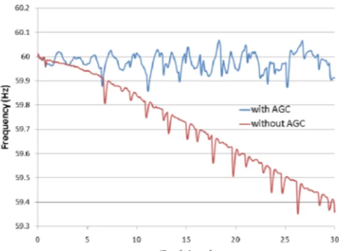
Simulation results show that current AGC settings are accurate and keep frequency near its nominal value. The largest deviation is slightly more than 0.2 Hz. Fig. 5 shows the benefits with AGC (blue curve) compared to the red curve showing the frequency decreasing without AGC.
Fig. 5. AGC impact for network frequency regulation: 3500 MW wind farms scenario.
Frequency oscillations are caused by the AGC. The first 5 seconds of the blue curve show oscillations caused by AGC delays and dead bands. Without AGC the frequency is more linear but the governors themselves cannot bring back the frequency to 60 Hz. In this case, the frequency drops to 59.4 Hz. The spikes are due to automatic switching shunt reactors who suddenly raise the voltage profile.
Fig. 6 shows the total wind generation for the 3500 MW wind integration. The initial generation is about 2900 MW (Pref). The generation pattern used is a ramp from 100 % of
Pref to 75% of Pref after 30 minutes, which gives a linear
variation.
Fig. 6. Total generation variation for the 3500 MW wind farms simulation (25% lowering ramp).
Voltage at Rimouski 315 kV bus is shown in Fig. 7. In this case, the WFMS raises voltage of Gaspésie area. At initialization, the voltage at Rimouski is higher with the WFMS. After a few seconds, the WFMS rapidly increases the voltage to its nominal value.
Fig. 7. Voltage at Rimouski substation, 315 kV bus for the 3500 MW planned for 2015.
In conclusion, 3500 MW of wind farms will not be a problem for frequency regulation with actual AGC settings. In fact, variation of 3500 MW is less than DC interconnection variation (up to 1500 MW in 10 minutes). Nonetheless, simultaneous variation of both can happen. Combining wind forecast and scheduled area interchange shall be considered.
B. Exploration for 10 000 MW of Wind Farms in Hydro-Québec Network
When it comes to integrating more wind farms, an important question arises: what is the maximum wind power that HQ can integrate? One says that the more disperse wind farms are, the more the generation is flattened [7].
The simulations of the previous section (load variation of 4000 MW) were repeated, but with 10 000 MW of wind farms. With the current network (40 000 MVA), 10 000 MW means 25% of wind power. Generation was scaled in Beauce, Charlevoix and Montréal areas. Generation in Gaspésie stays at 2150 MW and a new wind farm is added near the Chibougamau substation (see map in appendix). Enough spinning reserve was initially set to simulate generator start up. Also, voltage at 735 kV buses is regulated by switching numerous shunt reactors. Once again, simulations assume that network operators can keep the voltage within the normal range.
Fig. 8 shows that actual AGC settings are adequate to control the frequency; the maximum deviation is 0.25 Hz. However, as spinning reserve goes down, the AGC becomes more oscillating. The 500 MW minimum might be increased to let the AGC regulate frequency.
Fig. 8. Network frequency for the 10 000 MW scenario
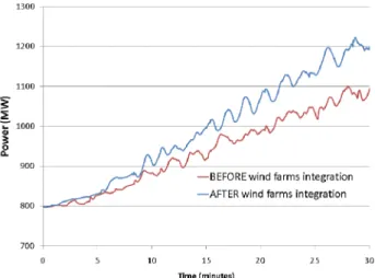
Fig. 9 shows mechanical power for one of the 13 power plants available to AGC before and after wind farms. Oscillations due to wind farm integration are caused by AGC. High gain in PI controller gives a fast frequency recovery but brings power oscillations. For the moment, those oscillations are still acceptable.
Fig. 9. Before and after wind farms integration - Power at Manic 3 plant.
Simulation results show that AGC settings must be reviewed with a large amount of wind turbines. Stability studies with the AGC will be required to monitor wind farm integration. Furthermore, dynamic behavior of the system frequency due to first contingency production loss will also be reassessed. Optimum settings of speed governors and AGC setting will be crucial for proper frequency regulation.
IV. FUTURE DEVELOPMENT
The next development for wind farm integration studies will include voltage stability studies, fault sensitivity and inertial response.
In 2015, most of HQ installed wind farms will be Type III & IV wind turbines. Those wind turbines can manage Low
Voltage Ride Through (LVRT) and will include Inertial Response controllers. QSS models need to be developed to perform those simulations.
Also, field tests and simulations of recorded events will contribute to specify modeling needs.
V. CONCLUSION
This paper deals with the wind integration and AGC frequency dynamics simulations using Quasi Steady-State approximation. Simulations include a complete AGC model, machines inertia and governors to represent frequency dynamics. For voltage dynamics, Wind Farm Management System in combination with machines exciters, static var compensator, synchronous condenser, tap changer transformers and automatic switching shunt reactors are also represented.
With QSS approximation, a 30 minute scenario takes only 60 seconds to simulate. This way, HQ can handle numerous simulations to optimize its AGC settings.
Simulations were made on two levels of wind integration: 3500 and 10 000 MW. Simulations take into account the worst combined effect of: load level, wind farms generation variation, area interchange variation and load following.
Results for the 3500 MW scenario show no particular misbehavior. Actual AGC settings are accurate and no excessive power oscillations are observed. There is no need to modify AGC settings or operating procedures. Local voltage is well regulated by WFMS. For the 10 000 MW of wind farms scenario, AGC regulates frequency properly if enough power is available. Minimum spinning reserve available to AGC might need to be raise in accordance with wind power generation. Otherwise, when it comes close to the 500 MW minimum criteria, frequency oscillations increase. Also, voltage regulation will be an issue for HQ, not for sub-networks which will be controlled by WFMS, but for the main network. Major wind power variation will have a significant impact on the voltage.
Finally, new QSS models will represent Type III & IV wind turbines controllers as Low Voltage Ride Through and Inertial response.
VI. APPENDIX Gaspésie Charlevoix Beauce Montreal Chibougamau VII. REFERENCES
[1] G. Trudel, S. Bernard, G. Scott. “Hydro-Quebec’s defense plan against extreme contingencies”, IEEE Trans. on Power Systems, Vol. 14, 1999, pp.958-965
[2] I. Kamwa, A. Heniche, M. de Montigny, “ Assessment of AGC and Load-Following Definitions for Wind Integration Studies in Québec,” 8th Integration Workshop on Large-Scale Integration of Wind Power into Power Systems as well as on Transmission Networks for Offshore Wind Power Plants, 2009.
[3] M. de Montigny, A. Heniche, I. Kamwa, R. Sauriol, R. Mailhot, D. Lefebvre, “A new simulation approach for the assessment of wind integration impacts on system operations” 9th Integration Workshop on Large-Scale Integration of Wind Power into Power Systems as well as on Transmission Networks for Offshore Wind Power Plants, 2010. [5] M.-E. Grenier, D. Lefebvre, T. Van Cutsem, “Quasi steady-state
models for long-term voltage and frequency dynamics simulation”, Proc. IEEE Power Tech conference, St Petersburg (Russia), June 2005 [6] Van Cutsem T., Grenier M.-E. & Lefebvre D. “Combined detailed and
quasi steady-state time simulations for large disturbance Analysis”,
International Journal of Electrical Power & Energy Systems, 28(9),
2006, pp. 634-642.
[7] F. Vallee, J. Lobry, O. Deblecker “Solutions to reduce the impact of wind prediction errors on the classical electrical park operation”, International Conference of Clean Electrical Power, 2009, pp. 248-252.
VIII. BIOGRAPHIES
Simon Lebeau received his B.Eng. degree in Electrical Engineering from École Polytechnique, Montréal, in 2001. He is with the Hydro-Québec TransEnergie Division where is involved in operations planning for the Main Network. He is a registered professional engineer.
Niko Qako received his B.Eng degrees in Electrical Engineering from University of Tirana (AL) in 1979 and PhD in Electrical Enginering from Ecole Polytechnique de Grenoble (FR). Since 2000 he works in IREQ-Hydro-Québec. Actually, his occupation is voltage stability domain
Thierry Van Cutsem (F’05) graduated in Electrical-Mechanical Engineering from the Univ. of Liège (Belgium), where he obtained the Ph.D. degree and he is now adjunct professor. Since 1980, he has been with the Fund for Scientific Research (FNRS), of which he is now a Research Director. His research interests are in power system dynamics, stability, security, simulation and optimization, in particular voltage stability and security.