Efficient FPGA Implementation of Gaussian Noise Generator for Communication Channel Emulation

HAL Id: hal-00347213

https://hal.archives-ouvertes.fr/hal-00347213

Submitted on 18 Dec 2008

HAL is a multi-disciplinary open access

archive for the deposit and dissemination of

sci-entific research documents, whether they are

pub-lished or not. The documents may come from

teaching and research institutions in France or

abroad, or from public or private research centers.

L’archive ouverte pluridisciplinaire HAL, est

destinée au dépôt et à la diffusion de documents

scientifiques de niveau recherche, publiés ou non,

émanant des établissements d’enseignement et de

recherche français ou étrangers, des laboratoires

publics ou privés.

Efficient FPGA Implementation of Gaussian Noise

Generator for Communication Channel Emulation

Jean-Luc Danger, Adel Ghazel, Emmanuel Boutillon, H. Laamari

To cite this version:

Jean-Luc Danger, Adel Ghazel, Emmanuel Boutillon, H. Laamari. Efficient FPGA Implementation of

Gaussian Noise Generator for Communication Channel Emulation. 7th IEEE International Conference

on Electronicsm Circuits & Systemes (ICECS’2K), Dec 2001, Kaslik, Lebanon. pp.1. �hal-00347213�

EFFICIENT FPGA IMPLEMENTATION OF GAUSSIAN NOISE

GENERATOR FOR COMMUNICATION CHANNEL EMULATION

Jean-Luc Danger

, Adel Ghazel

, Emmanuel Boutillon

, Hédi Laamari

(1)_{Ecole Nationale Supérieure des Télécommunications, ComElec, 46 rue Barrault, 75634 Paris Cedex 13, France}

(2)_{UTIC - Ecole Supérieure des Communications, Rte de Raoued km 3.5 – 2083 El Ghazala –Tunisia}

(3)_{LESTER, University of Bretagne Sud, 56321 Lorient Cedex, France}

danger@enst.fr, adel.ghazel@supcom.rnu.tn, emmanuel.boutillon@univ-ubs.fr

Abstract:

1 Introduction

Fast prototyping of digital communication systems needs efficient tools for the evaluation of the performance of the transmission algorithms. For example, to obtain an

estimation of the Bit Error Rate of 10-6 ± 3.3%, 109

iterations have to be done. Since the number of parameters in a modern system can be very high (sampling frequency, digital format, carrier resolution, rounding and quantification,…), the search for an optimal compromise between performance and complexity is not trivial and, simulation is generally the last tool used to perform this task [4]. To avoid software delays inherent in a long simulation, hardware emulation is investigated in the research project carried out between ENST-Paris (France), SUP’COM (Tunisia), LESTER (France) and University of Toronto (Canada). The idea is to use an FPGA board to emulate the system. A synthetized model of the channel and a synthetized version of the algorithms is used to perform measurement performance at very high speed. The main difficulty in emulating the channel, is to have an accurate Additive White Gaussian Noise (AWGN) generator, i.e.:

• B bits (2 to 10) of resolution after the decimal point

• a normal distribution up to more than 4 times the

standard deviation σ with a relative error less than

0.1% compared to the ideal distribution;

• a periodicity greater than 1018 (or 260);

• a flat spectrum;

• high sample rate (> 10 MHz.).

A theoretical method to fit this requirement was proposed by the author in [5]. This paper focuses on the FPGA implementation (namely the FLEX10K or APEX20K of Altera [2]) of the AWGN generator in order to reproduce the architecture. The paper is organized as follows : Section 2 recalls briefly the method proposed in [5], Section 3 described the overall architecture of the AWGN generator, Section 4 shows the LFSR (Linear Feedback Shift Register) optimization and Section 5 gives the design results.

2. Design of accurate AWGN reference

model

The Gaussian noise sample is generated in two steps. First, a quantized version of the Box-Muller method is performed to obtain a good approximation of the Gaussian distribution. Second, several samples thus obtained are accumulated to generate the final sample. The aims of this last step is to smooth the fluctuaction of the distribution obtained with the quantized Box_Muller method (central limit theorem).

2.1. Box-Muller method

The Box_Muller method is widely used in software simulation. It generates a random sample n of gaussian

variable N(0,1) (zero mean and standard deviation σ=1)

from two uniformly distributed over [0,1] random

variable x1 and x2 using (see [3] for a proof) :

f(x1) =

−

ln(

x

)

g(x2) =

2

n = f(x1)g(x2) (3)

A quantized version of (1) and (2) using pre-computed values is proposed in [5]. It is based on a non-uniform quantization of segment [0,1] that allows very small

quantization is obtained by a recursive partition of segment [0,1]. Segment [0,1] is first partitionned in 16 sub-segments of same length, than the first sub-segment [0,1/16[ is then subdivided again into 16 sub-segments

and so on1_{. This operation is performed K times. K}

16-words ROM are used to store the quantized values of f(x) over each level of the partition using:

Fr(s) = R[2m f( r

s

16

δ

+

where r varies between 1 and K (level of partition), s

varies between 1 and 15 (sub-segment number) and δ, a

real number between 0 and 1, gives the sample position in the segment. Fr(s) is coded on 2+m bits, 2 for the

integer part to get to σ=4, m for the fractional part. R[x]

denotes the largest integer lower than x. The variable x1

is obtained using K 4-bit random generator rgr, r =1..K. The g(x) quantization is simplified using the symetries of the cosine function, the segment [0,1/4] is sub-divided into 256 sub-segments. Let us define s', an 8 bit random variable. g(x) is quantized as : G(s') = R

[

₂

512

δ'

s'

π

(

+

)

]

where δ' and m' have the same meaning as that of δ and

m of equation (5). G(s) is coded on 1+m' bits, 1 bit for

the integer part in order to get to 2, m' bit for the

fractional part. From the product:

P(r,s,s') = R[Fr(s)×G(s')×2B-m-m'_{] (6)}

The sign of the output sample n is obtained by using a random variable sign which complements P(r,s,s') when equal to 1 :

n = (1-2×sign) × P(r,s,s') - sign (7)

2.2. Mixed method

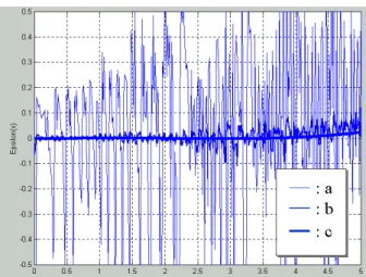
The curve a of figure 1 compares the distribution BM1 obtained with the parameters of Table 1 and the normal

distribution N(0,1) using the relative error ξX(x) :

ξX(x) =

)

(0,1)(

)

(0,1)(

−

ξ

ξ

N

N

x

X

(

)

Table 1: Characteristics of the Box-Muller AWGN To smooth the large variation of the distribution BM1, a number A of independant Box-Muller variables are

1_{Division in 16 sub-segments is done in order to optimized the design: the number}

of words in a Logical CELL (LCELL) is also 16 for a FLEX10K or APEX20K FPGA circuit.

accumulated (central limit theorem) to generate a single sample. The resulting distributions BM2 and BM4. obtained for A = 2 and 4 are shown in figure 1.

Figure 1: ξX(x) for X= BM1(a), BM2(b) and BM4(c)

Result of figure 1 shows that BM4 (curve c) fullfilled our initial requirement.

3. Overall architecture

As shown in figure 1, good results are obtained with K=5 and m=7, which means that (2+m)*K=45 logic cells are needed for the Fr ROMs. A 256-byte on-chip RAM can be used for the G ROM (m'=8-1=7). All these parameters correspond to Table 1 above. They are a good trade-off between performance and FPGA complexity.

Once the Box-Muller variable is generated a truncation can be done according to the needed accuracy to keep only B bits after the decimal point. In our example we truncated to get 6 bits after the decimal point. When the sign bit is one, the one's complement is used to get

negative values. Hence the mean value is now –2-B-1

instead of 0 before accumulation. After accumulation the mean and standard deviation are given by :

mean(BMA,B) = – A 2-B-1 (9)

standard deviation(BMA,B ) =

A

To be as close as possible to

N

to be done at the back end stage. The back end stage consists in multiplying the noise according to the needed SNR and in adding the result to the signal. For instance if A=4, a mere left shift of the decimal point is enough

to compensate σ and the addition with –2-B+1

compensates the mean.

Figure 2 represents the FPGA architecture with the 3 different blocks : the set of LFSRs to generate rgr, the Fr, G and sign functions for the Box_Muller variable and the accumulator for the central limit theorem.

The rgr generates the Fr ROM addresses. The address

from rgr is forced to 0 if one of the address from rg1 to

rgr-1 is different from 0. As the Fr (0)=0 (see equation 4),

this permits the use of an OR gate at the ROM output.

G Cos(x) Central limit Box-Muller X _ACCU sign 4 iter AWGN mult Truncation

L

F

S

R

+/-Figure 2: Architecture in FPGA

4. LFSRs optimisation

With this architecture, 29 uniformly distributed variables are necessary to generate the address bits of the 5 ROMs Fr (4 bits each), the ROM G (8 bits) and sign.

The use of LFSR is the classical technique to generate pseudo-random variables by using an irreducible polynomial [1]. Figure 3 illustrates the LFSR structure

called "one to many" with the polynomial x5 _{+ x}2 ₊₁

+

D Qx D Qx2 D Qx3 D Qx4 D Qx5 clk

Figure 3: LFSR for x5 _{+ x}2 ₊₁

The period and the number of combinations is 2n_{-1 if the}

LFSR has n registers. After Reset the LFSR has to be initialized with a value different from "00000" otherwise it stays in this state. Instead of using 29 LFSRs for the 29 variables, the number of LFSRs can be reduced if the address bits are grouped by packet of 4, necessiting only 7 LFSRs, 2 for the G ROM, one for each Fr ROM and one for the sign. At every clock cycle, 4 bits are use as outputs and "shifted". For instance for the LFSR of

figure 5, t being the clock period, the register x5 _{can be}

expressed as x5_{(t)= x}4_{(t-1) = x}2_(t-3)+x5_{(t-3) =}

x(t-4)+x4_{(t-4). By considering operations every 4t, 4 virtual}

shift operations are done in one clock cycle.

This technique can be easily coded in VHDL and generates almost no extra FPGA logic cells. The code of the LFSR function generator is given in the Annex for any number of outputs (parameter nb_iter in the code). Figure 4 illustrates the structure LFSR with polynomial

x5 _{+ x}2 _{+1 and 4 ouputs.} + D Q D Q x4 x5 clk D Qx D Qx2 D Qx3 + + + s₀ s₁ s2 s3

Figure 4: LFSR for x5 _{+ x}2 _{+1 and 4 outputs}

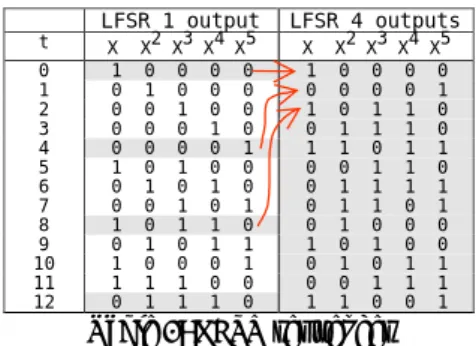
LFSR 1 output LFSR 4 outputs t _{X X}2 X3 X4X5 X X2X3X4 X5 0 1 0 0 0 0 1 0 0 0 0 1 0 1 0 0 0 0 0 0 0 1 2 0 0 1 0 0 1 0 1 1 0 3 0 0 0 1 0 0 1 1 1 0 4 0 0 0 0 1 1 1 0 1 1 5 1 0 1 0 0 0 0 1 1 0 6 0 1 0 1 0 0 1 1 1 1 7 0 0 1 0 1 0 1 1 0 1 8 1 0 1 1 0 0 1 0 0 0 9 0 1 0 1 1 1 0 1 0 0 10 1 0 0 0 1 0 1 0 1 1 11 1 1 1 0 0 0 0 1 1 1 12 0 1 1 1 0 1 1 0 0 1 Table 2: LFSR sequences

The sequence of the first 12 combinations of LFSRs of figure 3 and 4 is indicated in Table 2. The initial value is set to "00001". This table shows combinations of the 4-outputs LFSR correspond to every fourth combination of the 1-output LFSR.

In order to meet the periodicity constraint which is

greater than 1018 _{(or 2}60_{), at least a total of 60 registers}

of LFSRs are needed. In order to keep the highest period, the LFSRs need to have periods prime between them. To meet this condition, we propose to select the LFRS's length from the "Mersenne" numbers (number so

that 2d-1 _{is a prime number).}

5. Results

5.1 Accuracy

By considering the parameters of Table 1 and x between

0 and 4σ, the maximum relative error ξX(x) between the

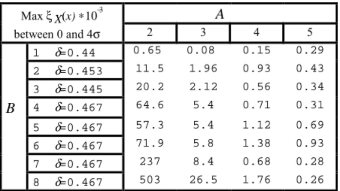
ideal gaussian distribution N[0,1] and the synthesized one is calculated by using the MATLAB model. The accuracy depends on B, which is the number of bits after the decimal point resulting from the truncation operation, and the number of accumulations A. Table 3

represents the maximum relative error expressed in 10-3

for different values of A and B. For every value of B the

A Max ξX(x) ∗10−3 between 0 and 4σ 2 3 4 5 1 δ=0.44 0.65 0.08 0.15 0.29 2 δ=0.453 11.5 1.96 0.93 0.43 3 δ=0.445 20.2 2.12 0.56 0.34 B 4 δ=0.467 64.6 5.4 0.71 0.31 5 δ=0.467 57.3 5.4 1.12 0.69 6 δ=0.467 71.9 5.8 1.38 0.93 7 δ=0.467 237 8.4 0.68 0.28 8 δ=0.467 503 26.5 1.76 0.26

Table 3 : maximum relative error for different A and B

5.2 Synthesis

Table 4 gives the results obtained with the parameters of Table 1, A=4, B=6 and LFSRs of length 22,21,20,17,13,7,5,15 registers for respectively G, Fr and sign :

FPGA device cells mem block clock rate Output rate 10K100ARC240-1 434 1 74MHz 18.5MHz 10K100EQC240-1 437 0.5 98MHz 24.5MHz

Table 4 : synthesis result

The synthesis has been done using FPGA ExpressTM and

MAX+PLUSIITM. The number of cells of the LFSR part

is 149. In order not to lose the performance level due to the 4 accumulations, 4 Box Muller generators can be placed in parallel and added in one shot. Consequently the hardware size is multiplied by 4. Figure 5 illustrates

the relative error obtained with 109 samples.

Figure 5: relative error with 109 samples

The difference between the theoretical distribution and the one obtained is due to the low number of samples

obtained for high value of σ. When the number of

samples increases the distribution converges towards the result of the MATLAB simulation

6. Conclusion

In this paper, a new technique for generating in real time gaussian noise and emulating a transmission channel was developped by applying the central limit theorem to a gaussian distribution generated by the Box-Muller method. Hardware in FPGA has been optimized by taking advantage of the logic cell structure and the on-chip RAM blocks. The proposed implementation delivers a quasi-perfect gaussian noise which has a

maximum relative error of 0.1% at 4 σ, compared to the

ideal distribution. The FPGA hardware uses only 8% of a 100K gates FPGA and can deliver a gaussian noise at 20MHz with a period which can last a few days at this frequency.

Reference

[1] J.G. Proakis, “Digital communications”, Mc

GRAW-HILL International Editions, Electrical Engineering Series, 1998.

[2] ALTERA Data Book 1998

[3] Donald E. Knuth, "The Art of computer

programming", ADDISON-WESLEY, 1998

[4] J.R. Ball, "A real time fading simulator for mobile radio", The radio and Electronic Engineer, Vol 52, N°10,October 1982

[5] A. Ghazel, E. Boutillon, J-L Danger, G. Gulak, H. Laamari, "Design and Performance Analysis of High speed AWGN Communication Channel Emulator", Paper submitted to ICC2001, Tampere Finland

Annex

VARIABLE pol_int : std_logic_vector(pol'length-1 DOWNTO 0); VARIABLE pol_gen : std_logic_vector(pol'length-1 DOWNTO 0); BEGIN CASE pol'length is when 22 => pol_gen := "0000000000000000000011"; when 21 => pol_gen := "000000000000000000101"; when 20 => pol_gen := "00000000000000001001"; when 17 => pol_gen := "00000000000001001"; when 13 => pol_gen := "0000000011011"; when 7 => pol_gen := "0000011"; when 5 => pol_gen := "00101"; -- x^5 + x^2 + 1 when 4 => pol_gen := "0011"; -- x^4 + x + 1 when 3 => pol_gen := "011"; -- x^3 + x + 1 when others => pol_gen := "11"; -- x^2 + x + 1 END CASE;

pol_int := pol;

iteration : FOR i in 1 to nb_iter LOOP IF en = '1' THEN

IF pol_int(pol'length-1)='1' THEN

pol_int := (pol_int(pol'length-2 DOWNTO 0)&'0') xor pol_gen;

ELSE

pol_int := (pol_int(pol'length-2 DOWNTO 0)&'0'); END IF;

ELSE pol_int := pol_int; END IF;

END LOOP; RETURN (pol_int); END gen_lfsr;