Fiscal Convergence and Municipal Reforms in the Montreal Metropolitan Region Between 1996 and 2011

(1)

Université de Montréal

Rapport de recherche

Fiscal Convergence and Municipal Reforms in the Montreal Metropolitan Region Between 1996 and 2011

Rédigé par

Maxime Leblanc Desgagné

Dirigé par Jean-Philippe Meloche

François Vaillancourt

Département de sciences économiques Faculté des arts et des sciences

(2)

1 Introduction

At the end of the 90’s, Québec’s government modified the institutional structure of the Montreal metropolitan region. Those changes led to the creation of the Communauté Métropolitaine de Montréal in 2001 and to the amalgamation of municipalities around Montreal, Longueuil and Terrebonne. After the election of a new government in 2003, a demerger process was initiated by the provincial government 1 leading in 2006 to the demerger of some municipalities on the Island of Montreal and the South Shore (in Longueuil), as well as the creation of agglomeration councils. The main goal of the first reform was to ensure a higher level of cohesion in the production of local public services in the metropolitan area all the while assuring the consolidation of the central city (Sancton, 2003); however, with the second reform, the institutional structure ended up almost as decentralized as it originally was. As mentioned by Sancton (2005), the amalgamation and the de-amalgamation made the arrangements for the governance of Montreal quite complex and unique, thus making it an interesting topic for further study.

This research evaluates how municipal institutional changes have affected the fiscal equity and efficiency in the production of local public services in the Montreal metropolitan region between 1996 and 2011. Firstly, we estimate the convergence of the fiscal effort between municipalities in the area considering three periods: the pre-merged, the merged and the post-merged periods. Secondly, the efficiency is subjected to a short analysis considering municipalities’ spending.

(4)

2 Literature Review

2.1 Regionalism and Localism

There are currently several academic papers on local public finance that are interested in institutional reforms and metropolitan governance. As noted by Hamilton et al. (2004) or Jiminez and Hendrick (2010), there is an ongoing debate between regionalists, in favour of metropolitan consolidation, and localists, who promote fragmentation. Both make use of models with similarities, but their underlying hypotheses differ. Moreover, empirical results are also inconclusive; depending on the context, they can be said to support both theories (Hendrick and al, 2011).

Most recent studies in the field of the economic impacts of consolidation or fragmentation of local governments examine cities in the United States. Only a few such studies concern themselves with cities in Canada (Sancton 2000; Kushner and Siegel 2005). Only one of those examines Montreal’s case. It is described in the next sub-section.

Two arguments are generally evoked to justify the implementation of a coordination structure at the regional level (Sharp, 1995). The first is that it enhances efficiency in the production of local public goods and services, and the second is that it improves fiscal equity.

Different methods of metropolitan coordination exist in Canada, from municipal mergers to the addition of a supra-municipal level (Sancton, 2005). In the wake of the merger’s failure, central-city decentralization and the addition of multiple administrative levels, like the MMC and the agglomeration councils, have increased the weight of bureaucracy in the production of local public services (Delorme, 2009). A direct consequence of this is a loss of efficiency.

It is not easy to ascertain the exact measure of the production of local public goods and services, because many of these services do not have market values. Hence, it is hard to evaluate the

(5)

production level or the productivity and its efficiency. When data is available, research can make use of the theory of microeconomics with the measure of the transformation of local input into local output (Agonso and Fernandes, 2007). However, this data is not available for the Montreal Metropolitan region. Then again, it is possible to study specific categories of spending per capita, like the total or administrative spending, or the ratio of the administrative spending to total spending, in order to measure the efficiency. Therefore, we make the assumption that the variation of efficiency can be reflected and measured indirectly by the variation of the administrative and total spending. We have to keep in mind that it is a very narrow measure of a real variation of productivity and therefore be careful with the interpretation and conclusions we might draw. Over the years following the mergers and demergers, the media and some political parties have often reported an excessive administration cost attributable to the modification and addition of entities in the municipal structure of Montreal; they are described in the next section. Their argument was that there are too many structures to efficiently manage the municipality, thus increases the administrative spending come into play, and this consequently increases the property tax to finance this specific spending, and not for public local goods and services. Thus, we will attempt to verify whether the merger or the demerger have had an impact on the size of the administrative spending in proportion to the total municipalities’ budget.

Equity is the second argument supporting the consolidation of metropolitan regions. A formal definition of equity in a local government is a fiscal arrangement that imposes equal liabilities on people who have the same ability to pay (Rosen and al, 1999). Moreover, the concept itself can be interpreted in many ways. The equity between territories doesn’t necessarily imply equity between individuals (Estèbe, 2004). In our study, we will focus on the equity between municipalities. Same as for efficiency, it’s almost impossible to measure equity directly. In our attempt to do so, we compare an innovative equity index taking into consideration the fiscal

(6)

burden and the total spending per capita between municipalities, which will be explained in the third section. In the literature, the fiscal burdens are generally for the total amount of tax paid by a person, but it can apply to a part of the public sector, the local government in our case, and can be defined as the burden of the entire local residential and business taxes. In the province of Quebec, it is the standardized global taxation rate (TGTU); that concept will be explained in section 3. More generally, the taxes are separated by payers for analysis; business or residential. Slack and Bird (2012) have found that amalgamation likely equalises the service level between municipalities, despite the fact that it implies an increase of the cost of providing public local services. Hence, it may be more expensive, yet it leads to a more equal supply of services. In this section, we try to verify whether the spending becomes more similar or not in the context of the merger and the demerger. The same authors found that in the region of Toronto, the amalgamation led to a reduction of the residential property taxes, but the question of the distribution of fiscal burden was not addressed.

As stated by the mayor of Montreal at the end of the 90’s, the goal of the mergers was to re-equilibrate the finances between his city and its neighbouring suburbs (Sancton, 2005). Nevertheless, the same argument was used for the demerger later on. However, it is interesting to consider how fiscal disparities evolved through the structural changes that occurred in Montreal metropolitan region between 1996 and 2011.

2.2 Structure of Municipalities in the Montreal Area

2.2.2 History

Sancton(2003) clearly explains the context of the structural changes in Montreal. The mayor Pierre Bourque, in power from 1994 to 2001, was in favour of mergers and thus played a significant role in the amalgamation of the city. He was more or less the only mayor of a city

(7)

subject to amalgamation that was in agreement with such an idea. He worked hard to make the merger happen, but suburbs were resisting, and for some municipalities (Westmount, for example), it was linked to the sensitive issues of linguistic minorities. Although there were protests, the mergers were implemented by a provincial law voted by the national assembly as put forward by the government of the Party Québécois in 2001(Bill 170). Because of that, it was impossible for all concerned municipalities to avoid amalgamation. Lucien Bouchard, the prime minister at the time, has pointed to the benefits of equalizing taxes and services across the new city (Sancton, 2003).

The municipal reform was implemented on January 1st, 2002. Later, in April of 2003, the Liberal Party of Quebec won the election with aid of the promise to hold citizen consultations on the territorial reorganization. Those consultations could allow, under certain conditions, to demerge some of the municipality. The first condition was that, within the former municipal borders, 10% of the registered voters had to sign a register supporting holding a demerger vote. The second was that a majority vote in favor of demerging representing at least 35% of the registered voter had to be reached in a referendum to lead to a demerger. Even though 282 municipalities organised a referendum in 2004 (because they met the first condition), and 22 had a result of a majority of voters for demergers, only193 municipalities in the metropolitan area recovered their independent status on January 1st 2006 (meeting the second condition), 15 on the Island of Montreal an 4 on the South Shore, around Longueuil.

Since then, no municipality has demerged. Hence, that gives us three distinct periods to study from 1996 to 2011. The first comprises the initial situation, where no municipality has merged or

2

http://www.mamrot.gouv.qc.ca/organisation-municipale/historique/consultation-sur-la-reorganisation-territoriale/registres/tableau-cumulatif/

(8)

demerged yet (1996-2001); the second is when all municipalities were merged (2002-2005), and the last is when some were still merged, while and others have demerged (2006-2011).

2.2.1 Research

One of the few analyses of the consolidation or fragmentation of municipalities in Montreal metropolitan area was carried out by Collin and Hamel (1993). This paper tries to identify fundamental differences, if any, between municipalities in their budgetary choices. At that time, the reforms of 1978-1980 had given municipalities in Quebec full decisional power over their tax rates and budget spending, so each one could provide a different supply of goods and services. This reform was in line with the Tiebout Model, where citizens are considered to vote with their feet (Tiebout, 1956). This model suggests that when a person is in the process of choosing a community where to live, the amount of public services provided by the local government and the matching tax rate will be chosen to match his/her preference pattern. The conclusion of the analysis of Collin and Hamel (1993) is that no voluntary budgetary differentiation is found in the Grand Montreal area between the 136 municipalities studied. Various reasons have been cited. First, unlike most American cities, Québec’s municipalities don’t have any power on social services and are highly constrained by Quebec school board on education, and hence cannot modify the supply of public goods and services in these fields as they wish. Second, the municipal fragmentation was a result of many factors, but also, most significantly, historical choices. Hence, we can conclude that despite the fact that the merging process can improve or deteriorate public local government’s finances, the choice can be based on different criteria. According to Collin and Hamel (1993), municipalities do not have the power to change their supply of services.

(9)

2.3 Convergence

The fiscal convergence breaks away from Tiebout (1956) to borrow its foundation from the economic convergence theory, usually linked to economic growth (Magrini, 2004). An incorporation of a measurement of fiscal effort replacing economic growth in these models makes it possible, from an equity perspective, to measure the effects of institutional changes that happened in Montreal in the 2000’s.

According to Annala (2003), state and local fiscal policies have converged over the past 20 years in the USA. Fiscal convergence refutes the Tiebout hypothesis stating that policies must differentiate over time to provide the right amount of goods and services to the local population. This article tests whether the fiscal policies among the USA states are becoming increasingly similar. This is achieved by testing both beta and sigma convergence, and it appears that there is evidence of convergence.

In the same line of thought, Skidmore and Deller (2008) build a model, which is consistent with macroeconomic growth, which predicts convergence in government spending. The idea is that government activity can be viewed as a certain type of investment, and similar to private investment, they have decreasing marginal returns. Hence, a big local government will get a lower return on spending than a small local government. Holding that assumption and variables of the model constant, higher levels of past government spending will lead to a slower rate of growth in current government spending and vice versa. In other words, government spending will converge over time. There exist a few reasons why it must converge. First, it has been shown that local government spending decisions are influenced by decisions made by nearby communities (Besley and Case, 1995). Second, intergovernmental transfers from state to local governments may accentuate the convergence; the state transfers a bigger amount to poor communities with

(10)

low spending and a smaller one to rich and spendthrift communities. In reality, this may be the case in the USA, but in the province of Quebec, municipalities finance themselves trough local taxes and have a small range of activities compared to their southern neighbours; consequently, this effect may not play a significant role in our study. In the United States, local governments rely on other governments for 40% of their revenue and most of government at the State level has the control over the source of revenue of the local government (Chernick and al., 2011). In the province of Québec, the municipalities obtain from transfers only 8% of their revenue.4

The first convergence measure used is the σ-convergence from Quah (1993). This convergence considers the dynamics of the distribution of the income level per capita and its distribution across countries. The idea behind this convergence is, in fact, quite simple; we observe the evolution of the coefficient of variation (CV). The CV gives a ratio of the standard-variation and the average. The value of the CV is directly proportional to the spread of the distribution around the average. . Therefore, the variation from year to year can indicate whether there is a convergence. The σ-convergence has been used to study the distribution of some fiscal variables in previous papers but not from a local point of view (see Table 1).

The second measure used is the β-convergence, taken from Baumol (1986) and Barro and Sala-i-Martin (1992). Baumol used a growth regression with the initial level of income as the explanatory variable of the growth rate of the GDP per capita. A negative correlation between the initial income and growth implies a tendency for poor countries to catch up. This concept has been applied to fiscal convergence analysis in previous studies, but not to local fiscal effort (Table 1). The rate of the β-convergence is obtained by regressing the initial value of the fiscal effort on the growth rate of the fiscal effort of a given period.

4_{http://www.mamrot.gouv.qc.ca/pub/finances_indicateurs_fiscalite/information_financiere/publications_electronique}

(11)

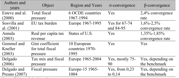
Table 1: Summary of research on fiscal convergence.

Authors and

years Object Region and Years σ-convergence β-convergence

Esteve and al. (2000) Total fiscal pressure 6 OCDE countries 1967-1994 Yes 2,4% convergence rate Sosvilla and

al. (2001) EU tax burden Europe 1967-1995 Yes for 67-74 and 84-95 1,6%-2,5% convergence rate Annala

(2003)

Real per capita tax revenue

States of U.S. Yes 1,35%-1,85%

convergence rate Gemmel and

Kneller (2003)

Gini coefficient for total fiscal pressure 10 European countries 1970-1995 Yes Yes Delgado

(2006) Tax mix and fiscal pressure Europe 1965-2004 Yes, mostly 75-90 Yes, depending on the benchmark Delgado and

Presno (2007) Fiscal pressure Europe-15 1965-1004 Yes, from 0,23 to 0,14 Yes, depending on the benchmark

Source: Table made by the author.

In our study we use these same concepts of convergence, but with a computed measure of fiscal effort called equity index. Based on the literature we analyzed, we are expecting that the amalgamations lead to a fiscal effort that is fairer, and the de-amalgamation has the opposite effect. This research will attempt to determine whether it is the case.

Even though both convergence concepts are strongly related, the β-convergence is considered a necessary, yet insufficient, condition for the narrowing of the distribution over time (Young and al. 2007). In other words, it is possible that the β-convergence happens when σ-convergence is not observed. This is why it is important to consider both measures in our analysis.

2.4 Efficiency

The efficiency in the production of local public services has been studied and reviewed in many articles. Martin and Hock Schiff (2011) have synthesized the methodology and the results on over fifty studies on the subject. In those studies, efficiency was a reduction of the cost for a same level of services or an improvement in the delivery of services. The general idea of the synthesis is that there are many studies that don’t finds any improvement of efficiency; some find a gain

(12)

and several find mixed results. Hence, there are no obvious conclusions to be drawn. Table 2 summarizes two empirical studies on amalgamation.

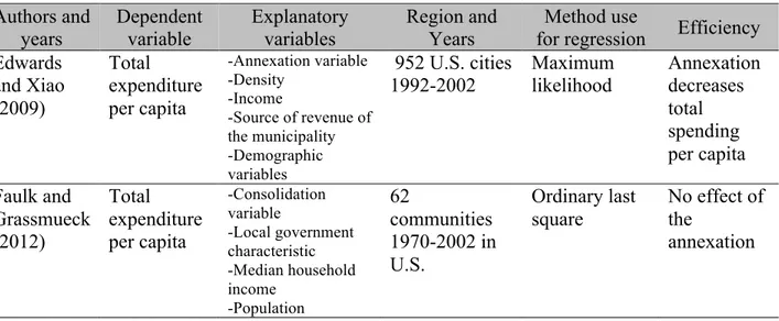
Table 2: Summary of research on efficiency with amalgamation of local government.

Authors and

years Dependent variable Explanatory variables Region and Years for regression Method use Efficiency Edwards and Xiao (2009) Total expenditure per capita -Annexation variable -Density -Income -Source of revenue of the municipality -Demographic variables 952 U.S. cities

1992-2002 Maximum likelihood Annexation decreases total spending per capita Faulk and Grassmueck (2012) Total expenditure per capita -Consolidation variable -Local government characteristic -Median household income -Population 62 communities 1970-2002 in U.S. Ordinary last square No effect of the annexation

Source: Table made by the author.

For our study, we will use an ordinary least square regression explaining the variation of the total spending per capita with explanatory variables, which can be found in Table 2. We do not expect to find a significant effect of the structural changes on efficiency.

3 Data and Methodology

3.1 Municipal Data for the Montreal Metropolitan Region

The database used in this study is constructed with financial data available from the Quebec Ministry of Municipal affairs (Ministère des Affaires municipales, des Régions et de l’Occupation du territoire du Québec – MAMROT), and also from financial reports produced by the municipalities and the boroughs. The territory analysed in this research refers to the actual Montreal Metropolitan Community (MMC). It comprises 3.7 million in 2013 residents over an

(13)

area of 4,360 km2. 5 We can see a representation of this territory on Map 1. It encompasses 82 municipalities and the central city, Montréal, is represented with an M. The data was collected on an annual basis from 1996 to 2011. For a few of the observations, an adjustment to make data comparable for every year is necessary due to the frequent structural changes and modifications of the accounting perimeter. The database is completed with socio-economic indicators from the Canadian censii of 1996, 2001, 2006 and 2011, with the Cansim dataset of Statistic Canada and the Québec’s Statistic Institute.

Map 1: Montreal Metropolitan Community in 2013

Source: Communauté métropolitaine de Montréal (www.cmm.qc.ca).

As mentioned in the previous section, the period studied goes from 1996 to 2011, and is divided in three phases. The first is the one before the reforms, and its span is from 1996 to 2001. The second period is characterized by the municipal mergers and the structure’s consolidation, and goes from 2002 to 2005. We adjust the data of the Canadian’s census of 2001 and 2006 to match

(14)

with the years of interest. Finally, the third period is the one where demergers occurred, from 2006 to 2011. The three periods will be referred to by their three final years, which are 2001, 2005 and 2011.

It was necessary to do a few adjustments to the data. First, all monetary amounts were converted in 1996 dollars using consumer price index of Statistic Canada6, so inflation does not affect ours results. Second, with the data from the MAMROT, some observations were missing in the data. For every missing observation we have done one out of two manipulations. If the data was between two observable years, we use the average of both of them. For the one in 1996 or 2011, it was preferable to have the exact same amount to the year before or after than calculates the variation between the observable data between 1997-2011 or 1996-2010, because of the structural changes that occur in many municipalities. Third, we only have 4 observations for the period between 1996 and 2011 from the Canadian census. We had to generate data for every year because there is no observation in the 2005 period. Hence, we have distributed the variation equally between two observations. This also applies to the data concerning employment and average personal income between 1996 and 2006, as well as in the 2006-2011 period. For example, if the employment is 100 in 1996 and 120 in 2001, we calculate 104 in 1997, 108 in 1998 and so on. Afterward, averages for the 3 periods were calculated. The data on the population is from the MAMROT, where annual data was available for every municipality. In Table 3, we can see the number of municipalities in the three periods. The actual number of municipalities in the first period is 106 but we have to drop 6 of them due to various reasons7, and this is also why we have 79 in the last period and not 82, the actual number in the MMC. The complete list is in Appendix 1, as are the reason why some of the municipalities were dropped.

6_{http://www.statcan.gc.ca/tables-tableaux/sum-som/l02/cst01/econ46a-fra.htm}

(15)

The number diminishes and after increases because between the two first periods, municipalities merge, and some of them demerge afterward.

Table 3: Distribution of the municipalities. Period Number of Municipalities

1996-2001 100

2002-2005 61

2006-2011 798

Source: MAMROT, 1996-2011.

3.2 The Measure of Fiscal Effort

The measure of fiscal effort is constructed with two variables, which will be used for the convergence of the fiscal effort afterward. The first one is the total spending index (SI). The total spending (S) is a sum of all the categories of spending by a municipality, which include spending on administration, security, hygiene, urban planning, leisure, health, and electricity. The average of the total spending weighted by population (P) has been calculated for every year (t) for all the municipalities (i). After the observed total spending of every municipality has been divided by the weighted average for a given year, we obtain the SI. The SI is one if the spending is equal to the average, and more/less than one if spending is superior/inferior to the average.

𝑆𝐼_!" = !!" !!"∗!!" ! !!! !!" ! !!! 𝑇𝐼_!" = !!" !!"∗!!" ! !!! !!" ! !!! (1)

Hence, this formula gives an indication of the magnitude of the spending compared to the weighted average. The second variable is the TGTU9 index (TI). The TGTU (T) stands for the standardized global taxation rate and is an indicator of the tax effort required by the municipalities standardized by the valuation of the taxable properties with their real values. In other words, the TGTU is the ratio of the income from taxes related to property over the assessment of taxable properties standardized to make it comparable between municipalities. The

8_{There are actually 19 demergers, and not 79-61=18, because we dropped l’Ile Dorval.}

(16)

TI index is built the same way as SI, in which the TGTU divided by the average of the TGTU weighted by the population for a corresponding year. The TI indicates the tax effort for a municipality compare to the average for a given year. The measure of fiscal effort is the equity index (EI). The EI is the ratio of TI on SI. An EI superior to one means that the tax effort is more important relative to its corresponding spending; the inverse situation yields an EI inferior to one.

𝐸𝐼_!" = !"!"

!"!" (2) Here’s an example for Montreal in 2001:

𝐸𝐼_{!"#$%&'(,!""#} = !,!" !,!"# !"##,!" !"!#,!" = 1,22 1,38= 0,88

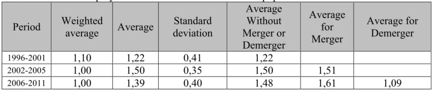
The interpretation of the 0,88 is that Montreal, in 2001, has a greater total spending compare to the average than it fiscal effort. We can see in Table 4 the average of the EI for the three periods. In the second column, the average EI is always superior to 1, which means that the fiscal effort over the average of the population’s fiscal effort is greater than the total spending on the average of the population’s total spending. We wanted to have two points of view in the initial and the second column; the first taking into consideration the size of the city, and the second, every city is equal in the analysis. The subsequent columns aren’t weighted by population. Montreal has a major impact in the weight because it accounts for more than 30% of the total population in the metropolitan area every year, and if we add Laval and Longueuil, this percentage goes up to 45%. Moreover, the standard deviation is getting low, and higher after, but it does not mean there isn’t convergence in the period itself. The three last columns present the separated average depending on the exclusive structural status of the municipality. Therefore, a municipality cannot be present in more than one of these three columns at the same time in a given period. However, municipalities can be grouped with merger, which means that the municipality has merged,

(17)

demerger, which means that the city has demerged, or neither. For the 2002-2005 period, the EI for the merged municipalities is similar to municipalities that haven’t had a structural change. For the 2006-2011 period, the average of the EI is higher for the merger and a lot lower for the demergers, and on average, it has reduced from the previous period. The 5 lowest and the 5 highest EI for the municipalities for every period are found in Appendix A. We can note that Montreal, once merged, is in the bottom five. It is the territory that has received most of the merged municipalities, and in the final period, both extremes contain demerged cities. Within the period, the distribution doesn’t change a lot, but it does change when the shocks of the merger and the demerger happen.

Table 4: Equity index between 1996-2011 for the population in the CMM area.

Period Weighted _average Average _deviationStandard

Average Without Merger or Demerger Average for Merger Average for Demerger 1996-2001 1,10 1,22 0,41 1,22 2002-2005 _1,00 _1,50 _0,35 _1,50 _1,51 2006-2011 1,00 1,39 0,40 1,48 1,61 1,09

Source: calculations by the author using data from MAMROT

The measure of fiscal effort presented here assumes that a fair distribution of spending among municipalities should be proportional to the resident population, which is denoted as the normal population. However, in a metropolitan context, some municipalities have a day population larger than their normal population since they are employment centers. Thus, spending in these municipalities will exceed resident population needs. In this case, a fair distribution of spending among municipalities should also consider the effect of day population. To do so, a second measure of fiscal effort has been computed. Assuming that the number of residents combined to the number of employees working in the municipality can take into account particularities of the

(18)

employment centers, which can more accurately reflect the number of users of public services in a municipality, we have:

𝐷𝑎𝑦 𝑝𝑜𝑝𝑢𝑙𝑎𝑡𝑖𝑜𝑛 = 𝑝𝑜𝑝𝑢𝑙𝑎𝑡𝑖𝑜𝑛 + 𝑒𝑚𝑝𝑙𝑜𝑦𝑚𝑒𝑛𝑡

You can find the 5 lowest and 5 highest proportions of the normal on the day population in Appendix A. A high proportion doesn’t demonstrate a lot of employment; therefore, a city with a high proportion is not an employment center. In general, the municipalities with high populations are employment centers. The data of the number of worker are taken from the Canadian’s census. The calculations for the equation (1), (2) and (3) where made for both populations, which is the 𝑃_!" that vary in (1) but has a repercussion to (2) and (3).

3.3 Measuring σ and β Convergence

The σ convergence and β convergence of the equity index can be measured to verify if the fiscal effort converges in each the three periods.

To calculate the variation over time of the dispersion of EI, the σ convergence is calculated with the mean (µ) and the standard variation (σ) of EI for every year. Accordingly, the coefficient of variation is calculated for every year, giving the σ convergence. It is the same idea of the economic convergence as used by Quah (1993), but applied to our measure of fiscal effort:

𝐶𝑉! = !_!!

!, (3) Moreover, we want to know, in every period, if there is a β convergence, which is the presence of a negative correlation between the initial value and the growth rate (Baumol, 1986). In other words, we want to verify if the initial value of the equity index relates to the magnitude of the growth rate in the subsequent year. Base on the model of Barro and Sala-i-Martin (1992), we will measure if there is β convergence, and if yes, at what rate. Assuming that 𝐸𝐼_!,! is our level of

(19)

local fiscal effort for the municipality i in year t, we can estimate the β convergence with the fallow equation:

ln !"!,!

!"!,! (1 𝑇) = 𝐴 − 𝐵 𝑙n(𝐸𝐼!,!) 𝑇 + 𝜀! (4) Where 0 and T represent the initial and the final year of each period, respectively, and 𝜀_! the error term. The regressions are made for the normal population and the day population. If B is significant in the regression, we can calculate the rate of β convergence resolving:

𝐵 = (1 − 𝑒!!"_{) (5)}

3.4 Measuring Efficiency

To validate if the mergers and demergers have affected the efficiency of municipalities, we assume that a loss (or gain) in efficiency can be measured by an increase (or decrease) of dollars spent on municipalities’ administrative costs. We will estimate regressions on two variables. The first variable is the growth rate of the administrative spending 𝐴𝑆_!, and the second is the growth rate of the total municipal spending 𝑇𝑆_!. Both variables are calculated in average for each period with the geometric average, with Z standing for each period; 2001, 2005 and 2011:

𝐴𝑆_! = !"!,! !"!,! ! − 1 , 𝑇𝑆_! = !"!,! !"!,! ! − 1. (6) Two ordinary last square regressions are estimated, one on 𝐴𝑆_!, and the other on 𝑇𝑆_!. The regressions are inspired by the works of Edwards and Xiao (2009) and Faulk and Grassmueck (2012), which look at the total local spending on explanatory variables, and here, we are looking at the growth rate of spending. They are estimated for the three periods Z with different models for each period. The first regression (7) verify if the variation of the administrative spending follow closely the variation of the total spending.

(20)

The dummy M is 1 if the municipality is amalgamated, and 0 in the contrary. The variable D is 1 if the municipality has demerged and recovered its autonomy or if the municipality has lost territory because other one left, like Montreal for example, and 0 otherwise. If M or D are significant, the variation of the administrative spending are affected by structural changes, this is probably due to a lost of efficiency or the cost of the change of the structure. We can see the distribution of the variables in table 5.

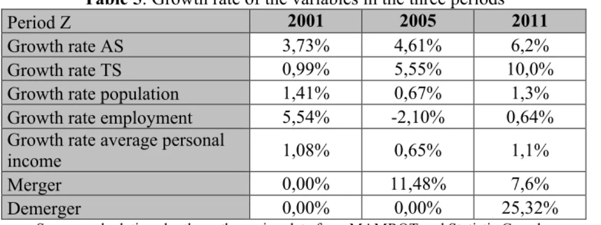
Table 5: Growth rate of the variables in the three periods

Period Z 2001 2005 2011

Growth rate AS 3,73% 4,61% 6,2%

Growth rate TS 0,99% 5,55% 10,0%

Growth rate population 1,41% 0,67% 1,3%

Growth rate employment 5,54% -2,10% 0,64%

Growth rate average personal

income 1,08% 0,65% 1,1%

Merger 0,00% 11,48% 7,6%

Demerger 0,00% 0,00% 25,32%

Source: calculations by the author using data from MAMROT and Statistic Canada

We can see that both AS and TS are increasing with each period, but this does not imply it must necessarily be due to the merger and demerger. The other variables vary in both direction from period to period. The Merger and the Demerger columns in Table 5 represent the share of the sample that has those dummies in each period.

The second regression (8) verifies if total expenditure growth follows characteristic of the population and is affected by mergers and demergers. The 𝐶_! is a vector of control variables including population growth rate, employment, and average revenue in 1996 dollars. These control variables are computed from census data from Statistic Canada. Regression equations are: 𝑇𝑆_!= 𝐴 + 𝐶_!+ 𝑀 + 𝐷 + 𝜀. (8)

(21)

From the literature we studied, we do not expect any particular effect on the efficiency measured on the growth rate of the total spending and the administrative spending. We think that spending will be mostly explained by the population variables.

4 Results

4.1 Convergence and Equity

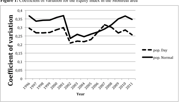
The σ-convergence for the equity index has been calculated and the results appear in Figure 1. Those figures present the evolution of the coefficient of variation of EI (cv) over time. A higher

cv means a wider spread of the distribution. Convergence (or divergence) is observed with the

decrease (or the increase) of cv over the period. The periods need to be commented separately because mergers and demergers were two exogenous shocks, and produce steps in the evolution of the cv. Keeping in mind that the solid line represents the normal population and the dotted line represents the day population, we can note that they demonstrate practically the same changes from year to year. But, interestingly, the cv level is lower when we take in consideration the employment.

(22)

Figure 1: Coefficient of variation for the Equity Index in the Montreal area

Source: calculations by the author using data from MAMROT and Statistic Canada

During the first period, 1996-2001, the cv varies little and there is no noticeable σ-convergence. Afterward, the shock of the merger is observed through a decrease of the cv, which attests to a fairer fiscal effort between municipalities. In the second period, the cv doesn’t change over the same period. It is interesting to note that we observe no significant shock in Figure 1 between 2005 and 2006, the second and the last period, because we could have expected one considering the shock between 2001 and 2002. Finally, in the 2005-2011 period, the cv tends to increase, although, the tendency is not clear. However, that aspect will be clarified in the next section. The results of the β-convergence of the equity index are found in Table 6, and the correlations of the regressions are in Appendix B.

0 0,05 0,1 0,15 0,2 0,25 0,3 0,35 0,4

Coef0ic

ien

t of variation

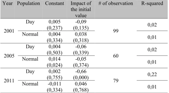
Year pop. Day pop. Normal

(23)

Table 6: Regression on the day population for β convergence by O.L.S.

Year Population Constant Impact of the initial value # of observation R-squared 2001 Day 0,005 (0,237) -0,09 (0,135) 99 0,02 Normal 0,004 (0,334) (0,318) 0,038 0,01 2005 Day 0,004 (0,503) -0,06 (0,339) ₆₀ 0,02 Normal 0,014 (0,024) -0,05 (0,374) 0,01 2011 Day 0,002 (0,755) -0,66 (0,000) 79 0,22 Normal -0,011 (0,334) 0,046 (0,768) 0,01

Source: calculations by the author using data from MAMROT. The () is the p-value.

The ordinary last squared regressions were estimated for each period and both populations. Regressions were robust, except day-2001 and day-2005, because they didn’t pass Breush-Pagan’s test at 5% (see Appendix C). A negative coefficient of the variable impact of the initial value means that a higher initial value is associated with a lower growth rate of the equity index, which signals convergence of the fiscal effort. If the coefficients are positive, it means divergence of the equity index, but it is not the case here.

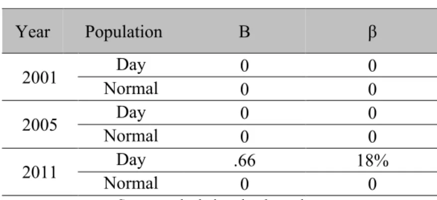
As for the σ-convergence, the first period doesn’t converge, nor is a β-convergence observable in the 2002-2005 period, when the mergers occurred. Both populations’ coefficients aren’t statistically significant. In Table 7, the annual rate of convergence of the fiscal effort, or the speed of convergence, is calculated, where the B column is the coefficient of the variable of Impact of the initial value in Table 6. In the last period, from 2006 to 2011, the coefficient isn’t significant for the normal population, but is at 1% for the day population. Therefore, the contradictory result for both populations makes the convergence unclear for this period. Thus, the annual rate of convergence stands between 0 % and 18% for this period. If we compare our

(24)

coefficient to the literature, it is slightly higher. This difference might be explained by the fact that these coefficients are associated to local fiscal effort, and not to state or national fiscal effort.

Table 7: B coefficient and convergence rate β

Year Population B β 2001 Day 0 0 Normal 0 0 2005 _NormalDay 0 0 0 0 2011 Day .66 18% Normal 0 0

Source: calculations by the author

With the results of convergence of fiscal effort, we can make conclusions on the impact on equity. What equity means for a municipality is the fact that it can set a tax rate proportional to its spending, which is the fiscal effort. For example, if a municipality has exactly the average tax rate in the metropolitan region but has only half of the spending compare to the average, it pays too much for what it gets. Hence, with both types of convergence, we know how the equity varies in every period. In the length of time for the first period, we can’t say that it become more equal or unequal. Perhaps if we had picked a longer period, we could have had a variation of the equity. Afterwards, the mergers had a strong impact on the distribution of the equity and reduced it. During the subsequent year, we can’t observe that it’s getting fairer with every year. The final year, when there are demergers, the equity is not clearly affected by the structural changes.

4.2 Spending and Efficiency

Two regressions were made to study the variations of the growth rate of the spending considering the structural changes in the municipalities.

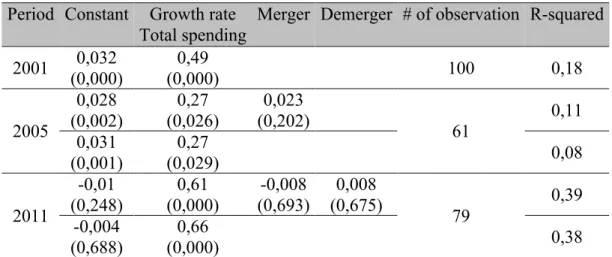
The results of the first regression concerning administrative spending appear in Table 8. The regression did not needed to be robust because they did pass Breush-Pagan’s test at 5% (see

(25)

Appendix C). It is the regression of administrative spending growth over total spending growth, with dummies for merged and demerged municipalities. Here, we try to identify whether the structural changes have an effect, in terms of increasing or a decreasing administrative spending growth rate. We can see in the results that the variable of the total spending is always significant at 1%, and is a major determinant of the growth of the administrative spending (refer to the correlation table in Appendix B). Moreover, there is no statistically significant effect of the merger or the demerger on the growth rate of the administrative spending.

Table 8: Regression on growth rate of administrative spending by O.L.S.

Period Constant Growth rate Total spending

Merger Demerger # of observation R-squared 2001 0,032 (0,000) 0,49 (0,000) 100 0,18 2005 0,028 (0,002) 0,27 (0,026) 0,023 (0,202) ₆₁ 0,11 0,031 (0,001) 0,27 (0,029) 0,08 2011 -0,01 (0,248) 0,61 (0,000) -0,008 (0,693) 0,008 (0,675) 79 0,39 -0,004 (0,688) 0,66 (0,000) 0,38

Source: calculations by the author using data from MAMROT and Statistic Canada. The () is the p-value.

The second regression is total spending growth over population’s variable with dummies for mergers and demergers, the results are in Table 9. The first and second regressions were robust because they didn’t pass Breush-Pagan’s test at 5% (see Appendix C). The regressions verify whether the variation of total spending relies on the structural changes of the municipality when population characteristics are taken into consideration. Our first observation is that most of the variables are not significant. Then, the merger variable isn’t significant in either of the second and third regression. Moreover, the last regression has demerger significant at 1%, and it means that the growth rate of the total spending is 9,3% higher for the demerged municipalities.

(26)

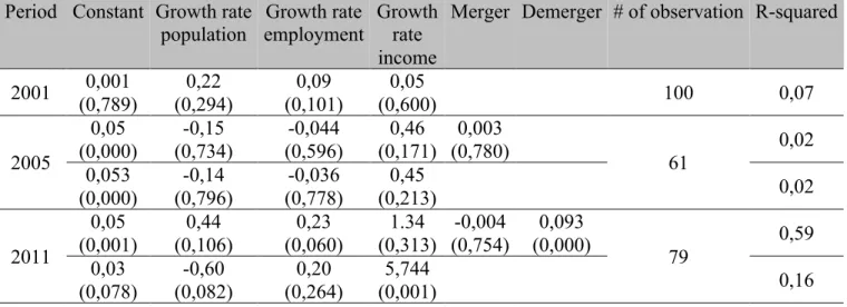
Table 9: Regression of growth rate of total spending by O.L.S.

Period Constant Growth rate

population employment Growth rate Growth rate income

Merger Demerger # of observation R-squared

2001 _(0,789)0,001 _(0,294)0,22 _(0,101)0,09 _(0,600)0,05 100 0,07 2005 0,05 (0,000) (0,734) -0,15 (0,596) -0,044 (0,171) 0,46 (0,780) 0,003 61 0,02 0,053 (0,000) -0,14 (0,796) -0,036 (0,778) 0,45 (0,213) 0,02 2011 0,05 (0,001) 0,44 (0,106) 0,23 (0,060) 1.34 (0,313) -0,004 (0,754) 0,093 (0,000) ₇₉ 0,59 0,03 (0,078) -0,60 (0,082) 0,20 (0,264) 5,744 (0,001) 0,16

Source: calculations by the author using data from MAMROT and Statistic Canada. The () is the p-value.

Our assumption was that a loss of efficiency due to structural changes could be measured through the spending growth rates of the municipalities. At first, we have verified that the merger or the demerger does not affect the growth rate of the administrative spending. In other words, we checked that the structural changes didn’t add additional administrative cost and didn’t affect the efficiency in that term. After that, it can be seen that the growth of the total spending wasn’t affected by the merger, but was by demerger. Hence, we can’t conclude that all structural changes affect the growth rate of the total spending. The demerged municipalities indeed have a higher growth in their total spending, but it does not mean that they are less efficient.

Those results are coherent with the literature. Martin and Hock Schiff (2011), in their synthesis on the efficiency of local government annexation, said that most of the empirical work on the matter hasn’t found strong evidence of an increase in the efficiency, which matches ours hypothesis.

(27)

5 Conclusion

The main objective of this research was to verify the existence of fiscal convergence in the Montreal area between 1996 and 2011, considering the structural changes that have occurred during this period. In addition, the growth rate of administrative and total spending were analysed to determine the effect of merger and demerger from the point of view of efficiency.

The results show that convergence of the fiscal effort did not occur after the merger, between 2002 and 2005. The results for the demerger are unclear, suggesting a potential convergence rate varying between 0% and 18% between 2006 and 2011. Furthermore, we didn’t find any clear evidence that structural changes affect the efficiency, as measured by unexplained growth in total spending.

Our results reinforce the conclusion of previous studies concerning institutional reforms at the local level. These reforms have little impact in terms of efficiency and equity for metropolitan areas. Future initiatives would do better if they focus on policies based on voluntary cooperation instead of compulsory amalgamation.

(28)

6 Bibliography

Afonso, Antonio, and Sonia Fernandes. 2007. Measuring local government spending efficiency: evidence for the Lisbon region. Regional Studies 40: 39-53.

Annala, Christopher N. 2003. Have state and local fiscal policies become more alike? Evidence of beta convergence among fiscal policy variables. Public Finance Review 31(2): 144-165. Barro, Robert J., and Xavier Sala-I-Martin. 1992. Convergence. Journal of Political Economy

100(2): 223-249.

Baumol, William J. 1986. Productivity Growth, Convergence, and Welfare: What the long-run data show. American Economic Review 76: 1072-1085.

Besley, Timothy, and Aanne Case. 1995. Incumbent Behaviour: Vote-Seeking, Tax-Setting, and Yardstick Competition. American Economic Review 85: 25–45.

Collin, Jean-Pierre, and Pierre J. Hamel. 1993. Les contraintes structurelles des finances

publiques locales : Les budgets municipaux dans la région de Montréal en 1991. Recherches sociographiques, 34(3): 439-467.

Chernick, Howard, Adam Langley and Andrew Reschovsky. 2011. Revenue diversification in large U.S. cities. IMFG papers on municipal finance and governance no.5.

Delorme, Pierre. 2009. Une île, une ville. Réunification ratée et complexification administrative. In Pierre DELORME (ed.). Montréal aujourd’hui et demain : Politique, urbanisme,

tourisme: 15-40

Edwards, Mary M. and Yu Xiao. 2009. Annexation, local government spending, and the complication role of density. Urban affairs Review 45: 147-165.

Estèbe, Philippe. 2004. Le territoire est-il un bon instrument de la redistribution ? Le cas de la réforme de l’intercommunalité en France. Lien social et Politiques 52: 13-25.

(29)

Faulk, Dagney, and George Grassmueck. 2012. City-county consolidation and local government expenditures. State and local government review 44: 196-205.

Gemmel, Norman, and Richard Kneller. 2003. Fiscal policy, growth and convergence in Europe. New Zealand treasury working paper 03/14.

Hamilton, David K., David Y. Miller, and Jerry Paytas. 2004. Exploring the Horizontal and Vertical Dimensions of the governing of Metropolitan Regions. Urban Affairs Review 40(2): 147-182.

Hendrick, Rebecca M., Benedict S. Jimenez, and Kamna Lal. 2011. Does Local Government Fragmentation Reduce Local Spending?. Urban affairs Review 47(4): 467-510.

Jimenez, Benedict S., and Rebecca Hendrick. 2010. Is Government Consolidation the Answer?. State and Local Government Review 42(3): 258-270.

Kushner, Joseph, and David Siegel. 2005. Are services delivered more efficiently after municipal amalgamations?. Administration publique du Canada 48 (2): 251-267.

Martin, Lawrence L., and Jeannie Hock Schiff. 2011. City-county consolidations: promise versus performance. State and local government review 43: 167-177.

Rosen, Harvey S., Paul Boothe, Bev Dahlby, and Roger S. Smith. 1999. Public finance in Canada, McGraw-Hill Ryerson.

Sancton, Andrew. 2000. La frénésie des fusions, une attaque à la démocratie locale. Ville de Westmount. McGill-Queen’s University Press: 205.

. 2003. Why municipal amalgamations? Halifax, Toronto, Montreal. Institute of Intergovernmental relations. Queen’s University.

. 2005. The governance of metropolitan areas in Canada. Public Administration and Development 25: 317-327.

(30)

Slack, Enid, and Richard Bird. 2012. Merging municipalities: Is bigger better?. In Moisi A. (Ed.). Rethinking local government: Essays on municipal reform. VATT Publications: 83-130. Sharpe, L. J. 1995. The Future of Metropolitan Government. In L. J. SHARPE (ed.). The

Government of World Cities: The Future of the Metro Model. John Wiley and Sons: pp. 11-32

Skidmore, Mark, and Steven Deller. 2008. Is Local Government Spending Converging?. Eastern Economic Journal 34: 41–55.

Skidmore, Mark, Hideki Toya, and David Merriman (2004), Convergence in Government Spending: Theory and Cross-Country Evidence, Kyklos, 57, pp. 587–619.

Tiebout, Charles M. 1956. A Pure Theory of Local Expenditures. Journal of Political Economy 64: 416-424.

Young, Andrew T., Matthew J. Higgins, and Daniel Levy. 2007. Sigma convergence versus beta convergence: evidence from U.S. county-level data. Journal of Money, Credit and Banking.

(31)

7 Appendix

7.1 Appendix A

Municipalities’ status of structural changes. (see legend at bottom).

Number Municipality's name 2001 2005 2011 Reason for X _population1996

1 Richelieu 3195 2 Saint-Mathias-sur-Richelieu 4014 3 Chambly 19716 4 Carignan 5614 5 Saint-Basile-le-Grand 11771 6 McMasterville 3813 7 Otterburn Park 7320 8 Saint-Jean-Baptiste 2913 9 Mont-Saint-Hilaire 13064 10 Beloeil 19294 11 Saint-Mathieu-de-Beloeil 2143 12 Brossard M D 65927 13 Saint-Lambert M D 20971 14 Boucherville M D 34989 15 Saint-Bruno-de-Montarville M D 23714 16 Longueuil M+ D- 127977 17 Greenfield Park M 17337 18 LeMoyne M 5052 19 Saint-Hubert M 77042 20 Sainte-Julie 24030 21 Saint-Amable 7105 22 Varennes 18842 23 Verchères 4854 24 Calixa-Lavallée 467 25 Contrecoeur 5331 26 Charlemagne 5739 27 Repentigny M+ 53824 28 Le Gardeur M 16853 29 Saint-Sulpice 3307 30 L'Assomption 11366

31 Saint-Gérard-Majella X X X Merged with

l’Assomption in 2000 X

32 Terrebonne M+ 42214

33 Lachenaie M 18489

34 La Plaine M 14413

(32)

36 Laval 330393 37 Montréal-Est M D 3523 38 Montréal M+ D- 1016376 39 Anjou M 37308 40 Lachine M 35171 41 LaSalle M 72029 42 Montréal-Nord M 81581 43 Outremont M 22571 44 Pierrefonds M 52986 45 Roxboro M 5950 46 Saint-Laurent M 74240 47 Saint-Léonard M 71327 48 Sainte-Geneviève M 3339 49 Verdun M 59714 50 L'Île Bizard M 13038 51 Westmount M D 20420 52 Montréal-Ouest M D 5254 53 Côte-Saint-Luc M D 29705 54 Hampstead M D 6986 55 Mont-Royal M D 18282 56 Dorval M D 17572 57 L'Île-Dorval X X X No population X 58 Pointe-Claire M D 28435 59 Kirkland M D 18678 60 Beaconsfield M D 19414 61 Baie d'Urfé M D 3774 62 Sainte-Anne-de-Bellevue M D 4700 63 Senneville M D 906 64 Dollard-des-Ormeaux M D 47826 65 Saint-Mathieu 1925 66 Saint-Philippe 3656 67 La Prairie 17128 68 Candiac 11805 69 Delson 6703 70 Sainte-Catherine 13724 71 Saint-Constant 21933 72 Saint-Isidore 2401 73 Mercier 9059 74 Châteauguay 41423 75 Léry 2410 76 Beauharnois M+ 6435

(33)

77 Maple Grove M 2606 78 Melocheville M 2486 79 Les Cèdres 4641 80 Pointe-des-Cascades 910 81 L'Île-Perrot 9178 82 Notre-Dame-de-l'Île-Perrot 7059 83 Pincourt 10023 84 Terrasse-Vaudreuil 1977 85 Vaudreuil-Dorion 18466 86 Vaudreuil-sur-le-Lac 28435

87 L'Île-Cadieux X X X No data on the _population X 88 Hudson X X X Too many data _missing X

89 Saint-Lazare 928 90 Saint-Eustache 11193 91 Deux-Montagnes 39848 92 Sainte-Marthe-sur-le-Lac 15953 93 Pointe-Calumet 8295 94 Saint-Joseph-du-Lac 5443 95 Oka - Municipalité 4930

96 Oka - Paroisse X X X Merged with Oka in ₁₉₉₉ X

97 Boisbriand 25227 98 Sainte-Thérèse 23477 99 Blainville 29603 100 Rosemère 12025 101 Lorraine 8876 102 Bois-des-Filion 7124 103 Sainte-Anne-des-Plaines 12908 104 Mirabel 22689 105 Saint-Pierre M 374

106 Notre-Dame-de-Bon-Secours X X X Merged with _{Richelieu in 2000} X Source: MAMROT between 1996-2011.

M=Merger, M+=the city received a new part of territory D=Demerger, D-=the municipality lost a part of territory X=the data was removed

(34)

Top 5 and Bottom 5 Equity Indexes for each period.

Period Ranking Name Merger Demerger EI population (in thousand)

1996-2001 Bottom 5 Montréal-Est 0 0 0,20 3,58 Westmount 0 0 0,26 20,32 Senneville 0 0 0,30 0,93 Dorval 0 0 0,34 17,45 Mont-Royal 0 0 0,40 18,31 Top 5 La Plaine 0 0 1,86 14,26 Saint-Amable 0 0 1,91 7,00 LeMoyne 0 0 1,98 5,32 Charlemagne 0 0 2,08 6,03 Pointe-Calumet 0 0 2,14 5,45 2002-2005 Bottom 5 Rosemère 0 0 0,82 13,92 Montréal 1 0 0,82 1852,48 Saint-Mathieu-de-Beloeil 0 0 0,89 2,29 Vaudreuil-sur-le-Lac 0 0 0,90 0,95 Mirabel 0 0 0,94 29,16 Top 5 Saint-Sulpice 0 0 1,96 3,57 Saint-Constant 0 0 2,01 23,60 Pointe-Calumet 0 0 2,28 5,83 Charlemagne 0 0 2,31 5,86 Saint-Amable 0 0 2,44 7,60 2006-2011 Bottom 5 Montréal-Est 0 1 0,34 3,85 Westmount 0 1 0,47 20,32 Dorval 0 1 0,69 18,30 Senneville 0 1 0,78 0,99 Rosemère 0 0 0,80 14,32 Top 5 L'Île-Perrot 0 0 1,98 10,14 Beauharnois 1 0 2,00 12,07 Saint-Amable 0 0 2,12 8,69 Dollard-des-Ormeaux 0 1 2,28 50,05 Pointe-Calumet 0 0 2,35 6,55 Source: calculations by the author using data from MAMROT and Statistics Canada

(35)

Top 5 and Bottom 5 Municipalities by periods of the normal population on the day population (in %)

Period Ranking Name Merger Demerger Normal population on day population 1996-2001 Bottom 5 Pointe-Calumet 0 0 0,95 Pointe-des-Cascades 0 0 0,95 Saint-Sulpice 0 0 0,93 Notre-Dame-de-l'Île-Perrot 0 0 0,93 Otterburn Park 0 0 0,92 Top 5 Senneville 0 0 0,49 Mont-Royal 0 0 0,49 Pointe-Claire 0 0 0,48 Montréal-Est 0 0 0,38 Dorval 0 0 0,32 2002-2005 Bottom 5 Pointe-des-Cascades 0 0 0,96 Pointe-Calumet 0 0 0,95 Otterburn Park 0 0 0,94 Calixa-Lavallée 0 0 0,93 Vaudreuil-sur-le-Lac 0 0 0,93 Top 5 Montréal 1 0 0,70 Mirabel 0 0 0,69 Delson 0 0 0,68 Saint-Mathieu-de-Beloeil 0 0 0,67 Contrecoeur 0 0 0,66 2006-2011 Bottom 5 Vaudreuil-sur-le-Lac 0 0 0,98 Pointe-des-Cascades 0 0 0,98 Pointe-Calumet 0 0 0,97 Otterburn Park 0 0 0,96 Saint-Philippe 0 0 0,95 Top 5 Mont-Royal 0 1 0,51 Baie d'Urfé 0 1 0,48 Montréal-Est 0 1 0,38 Senneville 0 1 0,34 Dorval 0 1 0,30

(36)

7.2 Appendix B

Correlation for the day population for β convergence

2001 2005 2011

In. Value In. Value In. Value

Av. Var. -0,15 -0,13 -0,47

Correlation for the normal population for β convergence

2001 2005 2011

In. Value In. Value In. Value

Av. Var. 0,10 -0,11 0,08

Correlation to verify efficiency for 3 periods.

2001 g.r.admin g.r.total g.r.pop g.r.empl g.r.income g.r.admin 1.0000

g.r.total 0.4214 1.0000

g.r.pop 0.2425 0.2095 1.0000

g.r.empl 0.1463 0.2124 0.2640 1.0000

g.r.income 0.0574 0.0148 0.1727 0.0496 1.0000

2005 g.r.admin g.r.total g.r.pop g.r.empl g.r.income merger g.r.admin 1.0000 g.r.total 0.2804 1.0000 g.r.pop 0.1249 -0.0375 1.0000 g.r.empl 0.1410 -0.0380 0.1453 1.0000 g.r.income 0.0182 0.1398 0.1522 0.0183 1.0000 merger 0.1548 -0.0197 0.2525 0.4468 0.0069 1.0000

2011 g.r.admin g.r.total g.r.pop g.r.empl g.r.income merger demerger g.r.admin 1.0000 g.r.total 0.7898 1.0000 g.r.pop -0.0525 -0.1013 1.0000 g.r.empl 0.0624 0.0899 -0.0872 1.0000 g.r.income 0.3353 0.2864 0.1220 -0.0305 1.0000 merger -0.1516 -0.1108 0.0188 0.2289 -0.0373 1.0000 demerger 0.6340 0.7267 -0.4184 -0.0092 0.3005 -0.1669 1.0000

(37)

7.5 Appendix C

Breush-Pagan’s test for the regression on the day population for β convergence by O.L.S. Period Population Prob > chi2

2001 Day _Normal 0.0114 _0.5678

2005 Day 0.0322

Normal 0.1633

2011 Day 0.5834

Normal 0.1027

Breush-Pagan’s test for the regression on growth rate of administrative spending by O.L.S. Period Regressions Prob > chi2

2001 0.0386

2005 With merger 0.0058

0.0047 2011 With merger and demerger 0.0000 0.0000