HAL Id: hal-00463825
https://hal.archives-ouvertes.fr/hal-00463825
Submitted on 15 Mar 2010
HAL is a multi-disciplinary open access
archive for the deposit and dissemination of
sci-entific research documents, whether they are
pub-lished or not. The documents may come from
teaching and research institutions in France or
abroad, or from public or private research centers.
L’archive ouverte pluridisciplinaire HAL, est
destinée au dépôt et à la diffusion de documents
scientifiques de niveau recherche, publiés ou non,
émanant des établissements d’enseignement et de
recherche français ou étrangers, des laboratoires
publics ou privés.
MyOwnLife: incremental and hierarchical classification
of a personal image collection on mobile devices
Antoine Pigeau
To cite this version:
Antoine Pigeau. MyOwnLife: incremental and hierarchical classification of a personal image collection
on mobile devices. IEEE Conf. on Multimedia and Expo (ICME’2008), Jun 2008, Hannover, Germany.
pp.873 - 876. �hal-00463825�
MYOWNLIFE: INCREMENTAL SUMMARIZATION
OF A PERSONAL IMAGE COLLECTION ON MOBILE DEVICES
Antoine Pigeau
LINA (CNRS FRE 2729), INRIA ATLAS group
2, rue de la Houssini´ere 44322 Nantes cedex 03 - France
firstname.lastname@univ-nantes.fr
ABSTRACT
In this paper, we propose a new method to summarize a per-sonal image collection, to provide a structure adapted to inter-face constraints on mobile devices. An incremental hierarchi-cal algorithm and a method of textual representation of each obtained event are proposed to build a geo-temporal classifi-cation. Results are validated with our prototype MyOwnLife on real data sets.
Index Terms— Personal image classification, mobile de-vice, hierarchical clustering
1
Goal and existing works
Building of personal multimedia collection is now wide-spread thanks to common mobile devices equipped with digital camera. Providing solutions to browse such a collec-tion is then a research area of much interest, requiring to deal with a large amount of data of different kind (audio, video and textual). Moreover, the difficulty of the task is increased on mobile devices due to their interface constraints. In this paper, we focus on personal image collections, which present the advantage on common image collections to have rich meta data, as time stamp and geographical information (from GPS system). The objective of our work is to provide summaries of the collection in order to facilitate the browsing task on a mobile device, a pertinent device to share/browse personal images due to its continuous availability.
The main steps of our approach are:
1.incremental building of a hierarchical temporal classifi-cation: we propose an improvement of our incremental and hierarchical algorithm [1], which provides a classification from the time stamp of each image. With our approach, we tend to emphasize the browsing task, rather than querying (a point motivated by the partial memory that the user has of the collection).
2.textual representation of obtained classes: each obtained class at the previous step is represented with a textual set of labels. The goal is to provide a succinct and simple repre-sentation of each event. Those summaries are built from new meta-data obtained from initial time stamp and Geographical Information System (GIS). The advantage of such approach
are the energy saving, since image displaying is costly. 3.combination of temporal and geographical informa-tion: to improve our hierarchical temporal classification, we propose a method to re-structure classes based on their ge-ographical information. Our approach consists in merging successive temporal nodes with similar geographical sum-mary (similar location based on a geographical map).
For existing automated schemes at research stage, time stamp has long been a favourite since it is an intuitively ap-pealing, cheap and reliable measurement. Segmenting the se-quence of time stamps has been viewed in [2, 3] as the incre-mental detection of gaps. Some thresholding sets the defini-tion of a ”meaningful” gap. But those soludefini-tions do not seem to provide hierarchical partitions in an unsupervised manner.
The work closest to the present paper is [4], which also organizes an image collection hierarchically, based on time and location clusters. To our understanding, their work in-corporates a series of rules derived from user’s expectations to build a geo-temporal hierarchy of events. Contrary to our work the number of levels in the hierarchy is set manually. Furthermore, their scheme is not incremental, but works in batch mode. In our view, incrementality is necessary to keep the collection organized without user help.
The remainder of this paper is organized as follows. Sec-tion 2 discloses the process to track a temporal hierarchy. Section 3 provides the building of a geo-temporal hierarchy. Finally, our approach is validated with experiments and the work is summarized in Section 4.
2
Temporal hierarchical partition
We opt here for a combination of a supervised clustering, for the finer partition, and the mixture model framework, for the
coarserpartitions (providing several summaries of the finer
partition). As in [4], we propose to set manually the precision degree of the finer partition fixing manually a boundary be-tween events.Such solution seems meaningful since it corre-sponds to the building process of a personal image collection [4], and provides a clear and robust initial partition to build the summaries. Each leave of our temporal tree is then an event with temporally connected images.
(a) 56000 5 10 15 20 25 5700 5800 5900 6000 6100 6200 6300 Number of merges ICL criterion local minimum (b)
Fig. 1. Selection of levels corresponding to local optima of the ICL
cri-terion: (a) the optimal ICL criterion found at each level of the binary tree represented on (b) is plotted. The grey rectangles indicate the corresponding selection of partitions. Once an optimum is found at a level q, we search for another local optima in each subtree from q. ’Local’ minima here is to be interpreted as follows: both slightly coarser and slightly finer partitions are worse, in the ICL sense.
build a hierarchical classification to provide several coarser summaries. Our approach is based on a mixture model frame-work. The main advantages is the availability of probabilistic criteria to select model complexities. The building of the sum-maries consists then in the following steps: (1) retrieve Gaus-sian model parameters from the finer partition (one GausGaus-sian component per initial classes), (2) apply a hierarchical algo-rithm [5], to provide a binary tree from a Gaussian model, and (3) select pertinent levels thanks to the Integrated Likeli-hood Criterion (ICL)[6], to avoid uninteresting and strongly redundant partitions. The ICL criterion provides a consistent solution to the issue.
q
binary tree 2
Selection of levels with ICL
Update of the main tree 3 4 Root q new node unchanged node nearest node 1 Root Build a new
Fig. 2.Update of a subtree: We add the new data group by the root, retrieve the model associated to its children and compute the likelihood of the new group based on the initial parameters. In this example, the new group is affected to the component q (the likelihood is higher than β and the choice of the node q is based on the MAP criterion). The update is then propagated to the node q: we retrieve the model associated to its children and compute the likelihood of the new group. Here we make the hypothesis that it is lower than β, we then update the subtree of root q. Fig. 2.1 presents the new node associated to the new group, its nearest node (here, the parameter Nnear= 1) and the unchanged nodes. We then re-build a binary tree from
the unchanged node, the leaves of the nearest node and the new node (fig. 2.2) and select the relevant levels based on the ICL criterion. Fig. 2.3 presents the obtained new subtree after our ICL selection. Finally the main initial tree is updated with the subtree (fig. 2.4).
As the process is incremental, the first step of our
algo-rithm is to group together new images with less than Tdif f
hours of time differences. Each group is then added by the root of our hierarchical classification and this node q is up-dated as follows:
1. If q is the root without any child, the group is added as a new child of q;
2. if q is a leaf, we add the new group in this node and the parameters of the tree are updated (from q to the root). 3. else:
3.1. detect the change due to the new image group: we retrieve the model composed of q’s children and compute the likelihood l of the new group based on the obtained parameter of the Gaussian model. If l > β, it means that the new group is associated with an existing cluster (selected with the MAP criterion) and we update this node (and re-iterate step 1); else
we add a new component qnew, a new child of q, associated
with the new image group and go to the next step;
3.2. search for summaries: we build a new binary tree
from the leaves of the Nnear nearest nodes of qnew and the
others children of q with the algorithm [5]. This agglomer-ative algorithm provides a binary tree from a Gaussian Mix-ture;
3.3. select the summaries in the obtained binary tree. This selection is carried out with the ICL criterion (fig.1);
3.4. merge the updated subtree with the initial one. Step 3(1) checks if the initial parameters fit its associated data including the new image group. The decision to add the new group in the current level or to propagate the update de-pend on the threshold β. A high likelihood for the new data involves that the parameters fit them well. The value of β is set manually: the higher β, the more distinct are the classes in the summaries (but the calculation complexity is increased).
The selection of the Nnear neighbours at step 3(2) attempt
to avoid poor summaries, due to the incremental property of our algorithm. Indeed a new group of images can have an influence on the whole tree (it could lead to a new coarser
summary). The parameter Nnearenables then to set the
num-ber of neighbours from which the search for new summary is carried out from the leaves (others nodes on the same up-dated level are also used but not from their leaves). The higher
Nnear, the higher are the quality of summaries and the
calcu-lation complexity. Figure 2 presents the different steps of our algorithm.
3
Geo-temporal partition
We present here a method to summarize a class with textual labels and then a technique to improve our temporal classifi-cation, combining it with geographical textual summaries.
Let us recall that the initial meta-data recorded with the mobile for each image are the time stamp and the loca-tion. Then a knowledge base can be used to provide user-meaningful information from the initial meta-data. Given a GPS coordinate, a GIS (Geographical Information System)
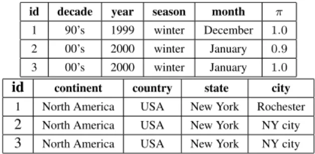
id decade year season month π 1 90’s 1999 winter December 1.0 2 00’s 2000 winter January 0.9 3 00’s 2000 winter January 1.0
id continent country state city 1 North America USA New York Rochester
2 North America USA New York NY city
3 North America USA New York NY city
Table 1.Example of attributes and values obtained respectively from the time stamp and the location.
could provide the continent, the country and so forth. Tables 1 present obtained temporal and geographical meta-data for 3 images, defined on 4 attributes in both cases. Notice that the attributes are organized in a hierarchical way.
First, an image i is defined by 2 temporal and geographi-cal sets of meta-data:
mi = {ht1, t2, . . . , tL|tl∈ Mti,
hs1, s2, . . . , sL0|sl∈ Msi}
where tl(or sl) is a textual label defined for the attribute l,
L (resp. L0) is the number of temporal (resp. geographical)
attributes to represent an image, according to the knowledge
base, and Mt and Ms are respectively the sets of possible
label values defined on temporal and geographical attributes. Then, we build the class summary with the textual sets as-sociated to its contained images. Let k be a class, its summary is defined as:
ck = {ht1, . . . , tl−1, {α1/t1l, . . . , αr/trl}i,
hs1, . . . , sl0−1, {α10/s1l0, . . . , αr0/sr 0
l0}i},
where tl∈ Mt, sl0 ∈ Ms, l and l0are the first attributes from
which label values present differences. For the attribute l (or
l0), the summary is represented by r (or r0) different values
associated to the contained images: α is the average weight of each textual label. This score, for both the temporal and spatial case, is the average of the image-to-class assignment π (see temporal Table 1) for each textual value:
αtr l = P i|tl r=tiπi Pnk i=1πi ,
where πi is the assignment probability of the image i to its
class and nk is the number of images in the class. Such an
approach enables to emphasize labels strongly associated to its class, labels which are likely to better represent its content. For example, if a class contains the images of Tables 1, its
class summaryis defined as:
c1= {h{
1
2.9 = 0.35/90’s,
1.9
2.9 = 0.65/00’s}i,
hNorth A., USA, NY, {0.35/Rochester, 0.65/NY city}i}
Here we have l = 1 and l0 = 3. The attributes Years and
Citiespresent different values.Stopping the textual summary
at attributes with different values enables to simplify their vi-sual representation and avoid building sets of labels that do not belong to the same time interval or location.
The same principle is applied to obtain the textual sum-maries of a node’s children, called level sumsum-maries. First we build the class summary of each child and then detect the at-tribute which presents different values among each summary. Each child is then only represented with the attributes with similar values until the first attribute with different values. For
example, let c2a class summary defined as:
c2= {h00’s, {0.42/2005, 0.58/2006}i
hEurope, France, ˆIle de F., {0.33/Paris, 0.66/NY city}i}
And let c1and c2two children of a node c, its level summaries
is then defined as:
cchildren(c1)= {h{0.33/90’s, 0.66/00’s}i, hNorth Americai} cchildren(c2)= {h00’si, hEuropei}
The summaries are limited to the Decade and Continent at-tributes. It enables to emphasize the main differences between events on a same level.
2 Root <00’s>, <North America> <00’s>, <Europe> <90’s>, <Europe> <00’s>, <Europe> <00’s>, <Europe> Root <00’s>, <Europe> <90’s, 00’s>, <Europe> <00’s>, <North America> temporal axis 1
Fig. 3.Figure 3.1 represents the initial temporal classification where each node is defined with its level-summary. Geo-temporal partition is then ob-tained by merging temporal continuous nodes with similar geographical sum-mary, as showed on fig. 3.2. Note that the merge step includes the update of the temporal summary of each obtained hybrid node (first node on fig. 3.2).
Fig. 4.Screen capture of our prototype MyOwnLife. Here, the hybrid view
is selected and the summary of the selected node in the tree is displayed: this node contains 2 events, each one represented by 2 images per each leave included in their subtree (thus, each event of the finer partition appears).
Finally, we propose a method to provide a hybrid partition of the image collection from the hierarchical temporal classi-fication. It follows the assumption that successive temporal events in a same location are generally connected. Roughly, the approach consists in merging continuous temporal nodes with similar geographical meta-data. Let q the root of the tree, our algorithm proceeds as follows:
1. get back the geographical level summaries of q;
2. for each continuous temporal classes i and j (children of q) with a similar geographical summaries: if i is a leaf and j a node (resp. j is a leaf and i a node) then move i as a new child of j (resp. j as a new child of i) else merge i and j (a new node containing the children of i and j).
3. apply step 2 to each child of q.
Practically, the obtained hybrid tree presents the property that each node on a same level are temporally and geographically disconnected: the gap between node is due to both a tempo-ral and a location change. Figure 3 presents a combination example of temporal and geographical views.
4
Experiments and conclusion
Experiments were carried out on four real user collections: G.B. (721 images taken over 4 years), C.C. (1731 images taken over 3 years) and S.P. (706 images taken over 4 years). All these collections contain images taken on several con-tinents (Asia, North America and Europe). For each col-lection, we built our hierarchical temporal classification, ask each user to annotate their obtained temporal events to build a geographical decision tree and finally build the geo-temporal
view based on the two previous classifications. Tdif f and
Nnearare set respectively to 3 hours and 2 nodes.
The temporal trees obtained for the collection of G.B., C.C. and S.P. are respectively composed of 5, 3 and 3 lev-els and are well-balanced. The number of children per node varies from 2 to 23. We notice that our classification extends in depth and width as new data are added. Only a minority of images implies serious restructuring of the tree, and hence the overall computational cost grows almost linearly with the number of images.
Bad Average Good Events/Leaves 0% 8% 92% Temporal Summaries 15% 24% 61% Geo-temporal summaries 0% 12.5% 87% Events/Leaves 5% 9% 86% Temporal Summaries 10% 40% 50% Geo-temporal summaries 6% 41% 53% Events/Leaves 9% 10% 81% Temporal Summaries 5% 17% 78% Geo-temporal summaries 3% 8% 89%
Table 2.Assessment of the events and summaries respectively for the S.P., C.C. and G.B. collections.
Our prototype MyOwnLife (see fig. 4) was then used to evaluate the obtained partitions. The prototype enables users to browse the different views (temporal, geographical or geo-temporal). The panel size containing images is similar to an Iphone screen : figure 4 is then a good example of how our proposal could enhance the browsing task on a mobile device: the events are clearly depicted and summarized with a limited number of images. Another solution could consist in mixing images and textual summaries.
To assess the improvement of the geo-temporal classifica-tion, we ask the users to give a mark to both events (leaves of the tree) and summaries (nodes of the tree). Results are reported in the Table 2. For each collection, we obtain a high
score for the events, due the small value of Tdif f: 81% −
92% of the leaves are considered as Good. The comparison between the temporal and geo-temporal tree shows that our combination of the temporal partition with the geographical textual summaries improves significantly the summaries (an average increase of 13.5% for the Good summaries). The Bad summaries are due to over-segmentations of connected events (connected events of some summaries are not regrouped in a same node) or under-segmentations (disconnected events in a same node).
This paper deals with the management of personal image collection on mobile devices. Our proposal is an algorithm to build a hierarchical and incremental classification, combining then with geographical meta-data, to provide a geo-temporal partition. We are currently examining solutions for a semi-supervised algorithm, taking into account user constraints on the structuring process.
5
References
[1] A. Pigeau and M. Gelgon, “Building and tracking hi-erarchical geographical & temporal partitions for image collection management on mobile devices,” in Proc. of Inter. Conf. of ACM Multimedia, Singapore, Singapore, Nov. 2005, pp. 141–150.
[2] A. Graham, H. Garcia-Molina, A. Paepcke, and T. Wino-grad, “Time as essence for photo browsing through per-sonal digital libraries,” in ACM Joint Conf. on Digital Libraries JCDL, Jun. 2002, pp. 326–335.
[3] J. C. Platt and B. A. Field M. Czerwinski,
“Photo-TOC: Automatic clustering for browsing personal pho-tographs,” Tech. Rep. MSR-TR-2002-17, Microsoft Re-search, Feb. 2002.
[4] M. Naaman, Y. J. Song, A. Paepcke, and H. Garcia-Molina, “Automatic organization for digital photographs
with geographic coordinates,” in Proc.of ACM/IEEE
Conf. on Digital libraries (JCDL), Jun. 2004, pp. 53–62. [5] C. Fraley, “Algorithms for model-based Gaussian
hierar-chical clustering,” SIAM Journal on Scientific Comput-ing, vol. 20, no. 1, pp. 270–281, 1999.
[6] C. Biernacki, G. Celeux, and G. Govaert, “Assessing a mixture model for clustering with the integrated classi-fication likelihood,” in IEEE Trans. on pattern analysis and machine intelligence, Jul. 2000, vol. 22, pp. 719–725.