1 INTRODUCTION
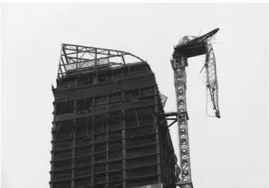
Tower cranes are designed to transport heavy weights. Over the last years, a large number of crane collapses has been recorded and massively reported in the media, e.g. in New-York in 2012 under storm Sandy (Figure 1). Many others are available on ded-icated websites (Christie, 2012) and (Mok, 2008).
Figure 1. Crane failure in New-York, 2012 (Christie, 2012).
Although the behavior of cranes is a widely stud-ied problem in the literature, most research works focus on the study of structures in use, i.e. during lift operations. The dynamic behavior of a crane lifting weights is studied by Ghigliazza by analogy with a pendulum with moving support (Ghigliazza &
Holmes, 2002) while the planning and modeling of the path traveled by the crane and its load are stud-ied in (Sakawa & Nakazumi, 1985) and (Hamalainen, et al., 1995) respectively. As tower cranes are high-rise and lattice structures, wind is an important excitation. In case of high wind velocities, the crane is out-of-service and left free to rotate as a weathervane in order to avoid overturning of the structure. The corresponding out-of-service wind speed is studied in (Eden, et al., 1981), (Eden, et al., 1983) and (Sun, et al., 2009). In opposition with all the previous research about tower cranes in use, Voisin performed experimental analysis in order to understand and characterize other crane instabilities under wind excitation and determine the susceptibil-ity of a tower crane to autorotation when it is out-of-service. This experiment consists in the determina-tion of a probability of autorotadetermina-tion of the jib in a given environment. This method allows to validate or not a configuration by experimental campaigns (Voisin, 2003) and (Voisin, et al., 2004).
A wide variety of tools already exists concerning wind loading, stochastic processes, dynamic analysis of structures and can be combined to analyze and better understand the behavior of tower cranes in a stochastic wind velocity field. A conceptual model of this problem will help catching the impact of the different geometrical, structural and wind parame-ters and their effect on autorotation. In this perspec-tive, the crane is represented by a single degree-of-freedom model composed of a rigid jib rotating around a fixed pivot (Vanvinckenroye, 2015). This
Stochastic rotational stability of tower cranes under gusty winds
H. Vanvinckenroye
Structural Engineering Division, Faculty of Applied Sciences, University of Liège, Liège, Belgium
V. Denoël
Structural Engineering Division, Faculty of Applied Sciences, University of Liège, Liège, Belgium
ABSTRACT: This work aims to study the rotational stability of a tower crane left free to rotate. Indeed, in case of important wind velocities, small oscillations can increase and build up into autorotations due to auto-parametric excitation of the structure. Many references in the literature describe the limit between oscillation and autorotation for simple cases like the deterministic pendulum and evidence the importance of the Hamil-tonian of a system on its stability. In this context the susceptibility of the structure to this dynamical instabil-ity is characterized by the average time necessary to reach a given energy barrier departing from an initial en-ergy level. This first passage time is the solution of the Pontryagin equation and is approached by an asymptotic expansion. First- and second-order terms are calculated as well as the boundary layer solution providing a correction when the initial energy is close to the barrier level.
mechanism is similar to a pendulum. As the wind loading depends on the angular position and velocity of the crane through aerodynamic forces and pres-sure coefficients, the wind excitation is called auto-parametric which is a characteristic of the pendulum as well. Assuming no damping, the dimensionless governing equation of this system submitted to an external force w(t) and a parametric force u(t) is given by:
𝑥̈ + (1 + 𝑢(𝑡)) sin 𝑥 = 𝑤(𝑡) (1)
Poulin studies the evolution of unstable regions for an excitation that varies continuously from peri-odic to stochastic (Poulin & Flierl, 2008). A wide variety of excitations are specifically tested in the literature. Gitterman studies the stability and the pe-riod of the pendulum under deterministic and sto-chastic excitation of its support in (Gitterman, 2010a) and (Gitterman, 2010b). He observes that an increasing stochasticity of the excitation induces larger, but of lower energy unstable ranges of pa-rameters.
Figure 2. Phase portrait of the non-excited Mathieu equation (Gitterman, 2010b).
The simplest case of a pendulum submitted to the vertical gravitational acceleration provides the ener-gy curves presented in Figure 2. Assuming no damp-ing, the pendulum will describe oscillations or rota-tions depending on its energy level H. Bishop, Garira, Xu and Clifford developed analytical solu-tions to approach the separatrix thanks to the har-monic balance method, the perturbation method and the critical velocity criterion (Garira & Bishop, 2003), (Clifford & Bishop, 1994), (Bishop & Clifford, 1996) and (Xu & Wiercigroch, 2006). Nar-row band and random phase excitations are investi-gated by Alevras and Yurchenko in (Yurchenko, et al., 2013) and (Alevras, et al., 2013) through a nu-merical path integration providing stability lobes when the support is submitted to a vertical harmonic excitation. Xu presents similar results in (Xu, et al., 2005) for a harmonically excited pendulum by evi-dencing the basins of attraction in the phase plane.
(Mallick & Marcq, 2004) present an analytical method providing an expression for the asymptotic probability distribution function of the energy.
This work aims to study the susceptibility of a crane to reach this instability zone when excited by Gaussian white noise excitations u(t) and w(t). If the stability is governed by the energy, i.e. the sys-tem is quasi-Hamiltonian, the probability of instabil-ity can be studied as the time needed to reach that critical energy level. As the excitation is stochastic, the first passage time is a random variable. An as-ymptotic expansion method was developed by Moshchuk in (Moshchuk, et al., 1995a) and (Moshchuk, et al., 1995b) to approximate the mean first passage time of a nonlinear stochastic process representing a ship motion on random sea waves. Chunbiao and Liu developed in respectively (Chunbiao & Bohou, 2000) and (Liu, et al., 2013) the stochastic averaging method for quasi-non-integrable-hamiltonian systems submitted to Gaussi-an Gaussi-and Poisson white noises Gaussi-and Li extended this approach to stochastic fractional derivative systems with power-form restoring force in (Li, et al., 2015). The first passage time can also be estimated through a multi-level Monte Carlo algorithm (Primozic, 2011). In this work, the asymptotic expansion is de-veloped for the linearized form of relation (1) taking the form of a stochastic Mathieu equation:
𝑥̈ + (1 + 𝑢(𝑡))𝑥 = 𝑤(𝑡) (2)
The quasi-Hamiltonian system is characterized by a set of Itô differential equations (Schuss, 2010) and the first passage time is obtained by solution of the corresponding Pontryagin equation (Moshchuk, et al., 1995a) and (Moshchuk, et al., 1995b). Finally, the accuracy of the expansion is illustrated by com-parison with Monte Carlo simulations of the motion.
2 AVERAGE FIRST PASSAGE TIME
The problem is governed by equation (2) where u(t) and w(t) are Brownian white noises of low intensity Su and Sw, and x is the rotational position of the
crane. This problem can be represented in the state space by its Itô formulation:
𝑑𝒙 = 𝒇(𝒙, 𝑡)𝑑𝑡 + 𝒃(𝒙, 𝑡)𝑑𝑩 (3)
where 𝒙 = (𝑞𝑝), 𝒇 = (−𝑞), 𝒃 = (𝑝 −𝑞0 01) and 𝑩 = (𝐵𝑢
𝐵𝑤) is the vector of Brownian motions u and w characterized by the intensity matrix
𝑺 = (𝑆𝑢 0
0 𝑆𝑤) = 𝜀𝝂 = ε (
𝜈𝑢 0
0 𝜈𝑤) (4)
As the white noise excitation is small, the system is quasi-Hamiltonian, which means that the Hamil-tonian of the system given by
H =p2
2 + 𝑞2
2 (5)
varies slowly in time.
The unperturbed system describes a closed trajec-tory of constant energy H called a homoclinic orbit. This motion presents a period
𝑇 = 2 ∫𝑞2𝑑𝑞𝑞̇ 𝑞1 = 2 ∫ 1 √2𝐻−𝑞2𝑑𝑞 = 2𝜋 √2𝐻 −√2𝐻 . (6)
The average first passage time through a level of energy Hc from an initial energy level H is the exit
time U(x) from a region 𝐷 = {(𝑥, 𝑥̇)|𝐻(𝑥, 𝑥̇) ≤ 𝐻𝑐}
and satisfies the Pontryagin partial differential equa-tion (7):
𝐿𝑈(𝒙) = −1 (7)
where L is the backward Kolmogorov operator and is given by (Schuss, 2010): 𝐿[∙] =1 2𝑻𝒓 {[ 𝜕 𝜕𝒙 𝜕 𝜕𝒙(∙)] 𝝈} + 𝒇(𝒙, 𝑡) 𝜕∙ 𝜕𝒙 (8)
where σ=εb(x,t)νbT(x,t). This operator can be
de-composed in two operators:
𝐿[∙] = 𝐿1[∙] + 𝜖𝐿2[∙]. (9) with { 𝐿1[∙] = 𝑝 𝜕∙ 𝜕𝑞− 𝑞 𝜕∙ 𝜕𝑝 𝐿2[∙] = 1 2(𝑞 2𝜈 𝑢+ 𝜈𝑤) 𝜕2∙ 𝜕𝑝2 (10) The first operator represents the derivative along the direction of the conservative system, i.e. along the homoclinic H.
The asymptotic expansion method developed by Moshchuk in (Moshchuk, et al., 1995a) and (Moshchuk, et al., 1995b) solves equation (7) for an approximate form of the first passage time:
𝑈(𝑝, 𝑞) ~ 𝑈𝑛(𝑝, 𝑞) + 𝐺𝑛(𝑝, 𝑞) (11)
where Un is the regular asymptotic outer solution
and is of the form 𝑈𝑛(𝑝, 𝑞) =
1
𝜖𝑢0(𝑝, 𝑞) + 𝑢1(𝑝, 𝑞) + ⋯ + 𝜖 𝑛−1𝑢
𝑛(𝑝, 𝑞) (12)
and Gn stands for the inner solution in the boundary
layer at the limit of the domain D so that LUn=-1
and LGn=0. This boundary layer solution will be
de-veloped with the second-order term u1.
Collecting terms of likewise powers of ε in rela-tion (7) yields:
𝐿1𝑢0 = 0 (13a)
𝐿1𝑢1+ 𝐿2𝑢0 = −1 (13b)
𝐿1𝑢2+ 𝐿2𝑢1 = 0 (13c)
2.1 Leading order solution
The leading order equation (13a) means that u0 is
constant along each homoclinic orbit and is conse-quently a function of the Hamiltonian H only.
The averaging along a period of Equation (13b) provides the information to determine u0(H). Indeed,
as the homoclinic orbits are closed, averaging along this curve gives zero and equation (13b) becomes
〈𝐿2𝑢0〉 = −1 (14a) 1 2[〈𝑞 2𝜈 𝑢+ 𝜈𝑤〉 𝑑𝑢0 𝑑𝐻 + 〈𝑝 2(𝑞2𝜈 𝑢+ 𝜈𝑤)〉 𝑑2𝑢 0 𝑑𝐻2] = −1 (14b)
where the following relations have been used for the partial derivatives: 𝑢0 = 𝑢0(𝐻) → { 𝜕𝑢0 𝜕𝑝 = 𝑝 𝑑𝑢0 𝑑𝐻 𝜕2𝑢0 𝜕𝑝2 = 𝑑𝑢0 𝑑𝐻 + 𝑝 2 𝑑2𝑢0 𝑑𝐻2 (15) and the operator 〈 ∙ 〉 represents the average over one period of the unperturbed motion:
〈 ∙ 〉 =2𝜋1 ∫02𝜋 ∙ 𝑑𝑡. (16)
The averaged second-order Pontryagin equation therefore reads: (𝐻 2𝜈𝑢+ 1 2𝜈𝑤) 𝑑𝑢0 𝑑𝐻 + ( 𝐻2 4 𝜈𝑢+ 𝐻 2𝜈𝑤) 𝑑2𝑢0 𝑑𝐻2 = −1, (17)
with the boundary conditions u0(Hc)=0 and
│U(0)│<∞, equation (17) provides the following solution: u0(𝐻) = 4𝜖 𝑆𝑢𝑙𝑜𝑔 ( 𝐻𝑐𝑆𝑢+2𝑆𝑤 𝐻𝑆𝑢+2𝑆𝑤). (18)
This solution presents two limit formulations when u(t) and w(t) are respectively equal to zero, 𝑆𝑢 → 0 ∶ 𝑢0 → 2𝜖
𝐻𝑐−𝐻
𝑆𝑤 (19a)
𝑆𝑤 → 0 ∶ 𝑢0 → 4𝜖log (𝐻𝑐)−log (𝐻)
𝑆𝑢 (19b)
2.2 Second order solution
As the leading order solution u0 is known, equation
(13b) is used to determine the second order compo-nent u1.
The variables q and p are changed into energy-phase variables k and θ assuming following expres-sions:
{𝑝 = 2𝑘 cos 𝜃
𝑞 = 2𝑘 sin 𝜃 (20)
so that the Hamiltonian H is now equal to 2k2.
Itô formulation (3) taking into account the Wong-Zakai correction terms δi detailed in (Schuss, 2010),
becomes: 𝑑𝒙∗ = 𝒇∗(𝒙, 𝑡)𝑑𝑡 + 𝒃∗(𝒙, 𝑡)𝑑𝑩 (21) where 𝑑𝒙∗ = (𝑑𝑘𝑑𝜃), 𝒇∗ = ( 𝜎22𝜕2𝑘 𝜕𝑝2 1 + σ22𝜕2𝜃 𝜕𝑝2 ) = ( 𝛿1 1+𝛿2),
𝒃∗ = (−𝑘 cos 𝜃 sin 𝜃
cos 𝜃 2
sin2𝜃 −sin 𝜃 2𝑘
) and the operators L1 and L2 become thanks to σ*=εb*(x*,t)νb*T(x*,t):
{𝐿1 [∙] = 𝜕𝜃𝜕∙ 𝐿2[∙] = 𝛿1 𝜕∙ 𝜕𝑘+ 𝛿2 𝜕∙ 𝜕𝜃+ 1 2𝜎11 ∗ 𝜕2∙ 𝜕𝑘2+ 1 2𝜎22 ∗ 𝜕2∙ 𝜕𝜃2+ 𝜎12∗ 𝜕2∙ 𝜕𝑘𝜕𝜃 (22)
Equation (13b) provides the following expres-sion: 𝐿1𝑢1= −1 − 𝐿2𝑢0= 〈𝐿2𝑢0〉 − 𝐿2𝑢0 (23) = 𝑘2𝜈 𝑢cos 2𝜃 𝑑𝑢0 𝑑𝐻+ (𝑘 2cos 4𝜃𝜈 𝑢− cos 2𝜃𝜈𝑤) 𝑑2𝑢 0 𝑑𝐻2
Integration of expression (23) with respect to θ provides a decomposition of u1 into two components
with the constant of integration u12(k):
𝑢1(𝑘, 𝜃) = 𝑢11(𝑘, 𝜃) + 𝑢12(𝑘) (24) with 𝑢11(𝑘, 𝜃) = 𝑘2𝑆𝑢sin 2𝜃 2(𝑘2𝑆 𝑢+𝑆𝑤)2((cos2𝜃− 2)𝑘 2𝑆 𝑢− 3𝑆𝑤). (25)
The averaging of equation (13c) over one period of the unperturbed motion provides:
〈𝐿1𝑢2〉+〈𝐿2𝑢12〉+〈𝐿2𝑢12〉 = 0 〈𝐿2𝑢12〉 = 1 16(𝑘 2𝜈 𝑢+ 𝜈𝑤) 𝑑2𝑢12 𝑑𝑘2 + 3𝑘2𝜈𝑢+𝜈𝑤 16𝑘 𝑑𝑢12 𝑑𝑘 = 0, (26)
and u12(k) takes the following form:
𝑢12(𝑘) =𝐶1𝜖
𝑆𝑤 𝑙𝑜𝑔 (
𝑘2𝜖
𝑘2𝑆
𝑢+𝑆𝑤) + 𝐶2 (27)
The first constant of integration C1 is equal to
ze-ro in order to respect the solvability condition │U(0)│<∞. The second constant C2 will be
de-termined together with the boundary layer solution in order to respect the boundary conditions.
2.3 Boundary layer
The boundary layer equation is:
𝐿𝐺𝑛 = 0 (28)
The coordinate stretching is classical in the boundary layers problems (Denoël & Detournay, 2010). The boundary layer solution Gn is written as a
function of the stretched coordinate ξ = (H-Hc)/√ε,
𝐺𝑛(𝜉, 𝜃) = 𝑔1(𝜉, 𝜃) + √𝜖𝑔2(𝜉, 𝜃) + ⋯ + 𝜖
𝑛−1
2 𝑔𝑛(𝜉, 𝜃). (29)
Similarly, the operator L is transformed via de Taylor expansion of the functions σi* and δi in the
neighborhood of H=Hc:
𝛿𝑖(𝐻, 𝜃) = 𝛿𝑖(𝐻𝑐, 𝜃) + √𝜖𝜉𝛿𝑖 (1)(𝐻
𝑐, 𝜃) + ⋯
𝜎𝑖∗(𝐻, 𝜃) = 𝜎𝑖∗(𝐻𝑐, 𝜃) + √𝜖𝜉𝜎𝑖∗(1)(𝐻𝑐, 𝜃) + ⋯ (30) The backward Kolmogorov operator becomes:
𝐿[∙] = 𝜕∙ 𝜕𝜃+ 4𝐻𝑐𝜎1 ∗(𝐻 𝑐, 𝜃) 𝜕2∙ 𝜕𝜉2 (31) + √𝜖 [[2√2𝐻𝑐𝛿1(𝐻𝑐, 𝜃) + 2𝜎1∗(𝐻𝑐, 𝜃)] 𝜕 ∙ 𝜕𝜉 + 2√2𝐻𝑐𝜎12∗ (𝐻𝑐, 𝜃) 𝜕2∙ 𝜕𝜉𝜕𝜃 + 4𝐻𝑐𝜉𝜎1 ∗(1)(𝐻 𝑐, 𝜃) 𝜕2∙ 𝜕𝜉2] + ⋯ = Λ0[∙] + √𝜖Λ1[∙] + 𝜖Λ2[∙] + ⋯
so that the governing equation (28) becomes: 𝐿𝐺𝑛 = (Λ0+ √𝜖Λ1+ ⋯ )[𝑔1+ √𝜖𝑔2+ ⋯ ]
= Λ0𝑔1+ √𝜖[Λ0𝑔2+ Λ1𝑔1] + ⋯ = 0 (32)
Balancing again the similar powers of ε provides the expression of the functions gi(ξ,θ). In particular,
the first order solution g1(ξ,θ) is the solution of the
following diffusion equation: Λ0𝑔1 = 𝜕𝑔1 𝜕𝜃 + 4𝐻𝑐𝜎1 ∗(𝐻 𝑐, 𝜃) 𝜕2𝑔1 𝜕𝜉2 = 0 (33)
with the boundary conditions g1(0,θ)=-u1(Hc,θ)
and g1(ξ,θ)→0 when ξ→-∞. The solution of this
equation is given by (Moshchuk, et al., 1995b): 𝑔1(𝜉, 𝜃) = b0+ ∑ 𝑏𝑛𝑒 √𝑛𝑐1 2 𝜉cos (𝑛𝛼(𝜃) − √𝑛𝑐1 2 𝜉) ∝ 𝑛=1 + ∑ 𝑎𝑛𝑒 √𝑛𝑐1 2 𝜉sin (𝑛𝛼(𝜃) − √𝑛𝑐1 2 𝜉) ∝ 𝑛=1 (34) with 𝑐1 = 2𝜋/ ∫ 4𝐻𝑐𝜎1∗(𝐻𝑐, 𝑠)𝑑𝑠 𝑇 0 𝛼(𝜃) = 𝑐1∫ 4𝐻𝑐𝜎1∗(𝐻𝑐, 𝑠)𝑑𝑠 𝜃 0 𝑏0 = − 1 2𝜋∫ 𝑢1(𝐻𝑐, 𝜃(𝛼))𝑑𝛼 2𝜋 0 𝑏𝑛 = −1 𝜋∫ 𝑢1(𝐻𝑐, 𝜃(𝛼)) cos(𝑛𝛼) 𝑑𝛼 2𝜋 0 𝑎𝑛 = −1 𝜋∫ 𝑢1(𝐻𝑐, 𝜃(𝛼)) sin(𝑛𝛼) 𝑑𝛼 2𝜋 0 (35)
Because of the second boundary condition, it fol-lows that b0=0 :
− 1
2𝜋∫ 𝑢1(𝐻𝑐, 𝜃(𝛼))𝑑𝛼 2𝜋
0 = 0. (36)
Finally, averaging (24) with respect to variable α, the constant of integration C2 is obtained:
〈𝑢12(𝑘)〉 = 𝐶2 = − 1
2𝜋∫ 𝑢11(𝐻𝑐, 𝛼)𝑑𝛼 2𝜋
0 = 0 (37)
Adapted to relation (35), only the even coeffi-cients an are non zero.
All in all, the solution including the first two terms is obtained as
𝑈 = 1
𝜖𝑢0+ 𝑢11+ 𝑢12+ 𝑔1 (38)
3 RESULTS AND CONCLUSION
Figure 3 presents the average first passage time of the energy barrier Hc=0.1 as a function of the initial
energy level for three different white noise intensi-ties of u and w. If Su=0, the relation is linear while
it is logarithmic if Sw=0. It can be observed from
re-lations (17) and (24) that the effects of u and w on the first passage time have the same order of magni-tude if Su has the same order as HcSw. This is
con-firmed in Figure 3. The results obtained with 2,000 Monte Carlo simulations are very close to the ana-lytical result obtained with first- and second-order expansion terms.
Figure 3. Comparison of theoretical (solid line) and simulated (dotted line) first-passage times with Hc=0.1 and θ=3π/4.
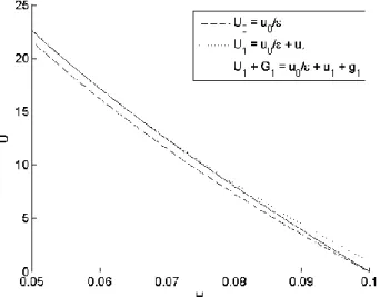
Figure 4 represents the contributions of the sec-ond-order term u1 as well as the boundary layer g1.
The second order term has a contribution independ-ent on the energy level H and the boundary layer is a correction on the second order term close to H=Hc
that keeps a first passage time equal to zero at this point.
Figure 4. Comparison of the first-order, second-order and boundary layer terms with with Su=0, Sw=0.001, Hc=0.1 and
θ=3π/4.
Finally, Figure 5 presents the boundary layer con-tribution in the (H,θ)-plane. The correction vanishes when the initial energy level H is getting away from the barrier Hc. Close to the barrier, the correction is
either positive or negative depending on the initial phase θ.
As a conclusion, the second order expansion pro-vides a concluding approximation of the first pas-sage time. Second order terms are of small order but the boundary layer contribution ensures the respect of the limit conditions.
(Vanvinckenroye, 2015)
Figure 5. Evolution of the boundary layer solution g1, with
Su=0, Sw=0.001 and Hc=0.1.
REFERENCES
Alevras, P., Yurchenko, D. & Naess, A., 2013. Numerical investigation of the parametric pendulum under filtered random phase excitation.
Bishop, S. & Clifford, M., 1996. Zones of chaotic behaviour in the parametrically excited pendulum. Journal of Sound and Vibration, 189(1), pp. 142-147.
Christie, L., 2012. craneaccidents.com. http://www.craneaccidents.com/2012/11/report/upda te/one57s-crane-problem/.
Chunbiao, G. & Bohou, X., 2000. First-passage-time of quasi-non-integrable-hamiltonian system. Acta Mechanica Sinica, 16(2), pp. 183-192.
Clifford, M. & Bishop, S., 1994. Approximating the Escape Zone for the Parametrically Excited Pendulum. Journal of Sound and Vibration, 172(4), pp. 572-576.
Denoël, V. & Detournay, E., 2010. Multiple scales solution for a beam with a small bending stiffness. Journal of Engineering Mechanics, 136(1), pp. 69-77.
Eden, J., Butler, A. & Patient, J., 1983. Wind tunnel tests on model crane structures. Engineering Structures, Volume 5, pp. 289-298.
Eden, J., Iny, A. & Butler, A., 1981. Cranes in storm winds. Engineering Structures, Volume 3, pp. 175-180.
Garira, W. & Bishop, S., 2003. Rotating solutions of the parametrically excited pendulum. Journal of Sound and Vibration, 263(1), pp. 233-239.
Ghigliazza, R. & Holmes, P., 2002. On the dynamics of cranes, or spherical. International Journal of Non-Linear Mechanics, 37(7), pp. 1211-1221.
Gitterman, M., 2010a. Spring pendulum: Parametric excitation vs an external force. Physica A: Statistical Mechanics and its Applications, 389(16), pp. 3101-3108.
Gitterman, M., 2010b. The Chaotic Pendulum. New Jersey: World Scientific Publishing.
Hamalainen, J., Virkkunen, J., Baharova, L. & Marttinen, A., 1995. Optimal path planning for a trolley crane: fast and smooth transfer of load. IEEE Proceedings - Control Theory and Applications, Volume 142, pp. 51-57.
Liu, W., Zhu, W. & Xu, W., 2013. Stochastic stability of quasi non-integrable Hamiltonian systems under parametric excitations of Gaussian and Poisson white noises. Probabilistic Engineering Mechanics, Volume 32, pp. 39-47.
Li, W. et al., 2015. First passage of stochastic fractinoal derivative systems with power-form restoring force.. International Journal of Non-Linear Mechanics, Volume 71, pp. 83-88.
Mallick, K. & Marcq, P., 2004. On the stochastic pendulum with Ornstein-Uhlenbeck noise. Journal of Physics A: Mathematical and General, 37(17), p. 14.
Mok, K., 2008. Youtube.com. YouTube - Crane
Spinning out of Control.
https://www.youtube.com/watch?v=0olg_j3289Q. Moshchuk, N., Ibrahim, R., Khasminskii, R. & Chow, P., 1995a. Asymptotic expansion of ship capsizing in random sea waves - I. First-order approximation. Int. J. Non-Linear Mechanics, 30(5), pp. 727-740.
Moshchuk, N., Khasminskii, R., Ibrahim, R. & Chow, P., 1995b. Asymptotic expansion of ship capsizing in random sea waves - II. Second-order approximation. Int. J. Non-Linear Mechanics, 30(5), pp. 741-757.
Poulin, F. & Flierl, G., 2008. The stochastic Mathieu's equation. Proceedings of the Royal Society A: Mathematical, Physical and Engineering Sciences, Volume 464, pp. 1885-1904.
Primozic, T., 2011. Estimating expected first passage times using multilevel Monte Carlo algorithm. University of Oxford: s.n.
Sakawa, Y. & Nakazumi, A., 1985. Modeling and Control of a Rotary Crane. Journal of Dynamic Systems, Measurement, and Control, p. 107:200.
Schuss, Z., 2010. Theory and Applications of Stochastic Processes - An analytical approach. Applied Mathematical sciences éd. New-York: Springer.
Sun, Z., Hou, N. & Xiang, H., 2009. Safety and serviceability assessment for highrise tower crane to turbulent winds. Frontiers of Architecture and Civil Engineering in China, Volume 3, pp. 18-24.
Vanvinckenroye, H., 2015. Monte Carlo simulations of autorotative dynamics of a simple tower crane model. s.l., Proceedings of the 14th International Conference on Wind Engineering, Porto Alegre.
Voisin, D., 2003. Etudes des effets du vent sur les grues à tour. PhD thesis éd. Ecole Polytechnique de l'Université de Nantes: s.n.
Voisin, D. et al., 2004. Wind tunnel test method to study out-of-service tower crane behaviour in storm winds. Journal of Wind Engineering and Industrial Aerodynamics, 92(7-8), pp. 687-697.
Xu, X. & Wiercigroch, M., 2006. Approximate analytical solutions for oscillatory and rotational motion of a parametric pendulum. Nonlinear Dynamics, 47(1-3), pp. 311-320.
Xu, X., Wiercigroch, M. & Cartmell, M., 2005. Rotating orbits of a parametrically-excited pendulum. Chaos, Solitons & Fractals, 23(5), pp. 1537-1548.
Yurchenko, D., Naess, A. & Alevras, P., 2013. Pendulum's rotational motion governed by a stochastic Mathieu equation. Probabilistic Engineering Mechanics, Volume 31, pp. 12-18.