Stéphane Polis
(F.R.S.-FNRS / ULiège)
17.04.2018
National Research University Higher School of Economics - Moscow
Plotting and exploring lexical semantic maps:
Resources, tools, and methodological issues
Semantic maps
Ø Two main types
o Connectivity maps
o Proximity maps (= MDS maps)
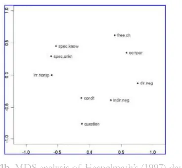
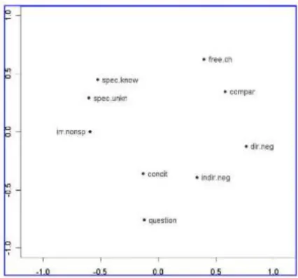
Figure 1b. MDS analysis of Haspelmath’s (1997) data on indefinite pronouns (Croft & Poole 2008: 15) Figure 1a. Haspelmath’s (1997: 4) original semantic
Le Diasema 3
Semantic maps
Ø Two main types
o Connectivity maps
o Proximity maps (= MDS maps)
Figure 1b. MDS analysis of Haspelmath’s (1997) data on indefinite pronouns (Croft & Poole 2008: 15) Figure 1a. Haspelmath’s (1997: 4) original semantic
map of the indefinite pronouns functions
o Graphs
• Nodes = meanings
• Edges = relationships between meanings
o Two-dimensional spaces
• Points = meanings (or contexts)
• Proximity = similarity between meanings (or contexts)
Le Diasema 5
Outline of the talk
Ø Different kinds of information captured by classical semantic maps
o Semantic closeness o Diachrony
o Frequency
Outline of the talk
Ø Different kinds of information captured by classical semantic maps
o Semantic closeness o Diachrony
o Frequency
o Types of semantic relationships
Ø Large-scale resources for lexical typology
o CLICS and CLICS 2.0 o Multilingual Wordnet
Le Diasema 7
Outline of the talk
Ø Different kinds of information captured by classical semantic maps
o Semantic closeness o Diachrony
o Frequency
o Types of semantic relationships
Ø Large-scale resources for lexical typology
o CLICS and CLICS 2.0 o Multilingual Wordnet
Ø Inferring classical semantic maps
o Regier et al. (2013)
o Weighted semantic maps o Diachronic semantic maps
Ø Exploring automatically-plotted semantic maps o Gephi
Le Diasema 9
Outline of the talk
Ø Different kinds of information captured by classical semantic maps
o Semantic closeness o Diachrony
o Frequency
o Types of semantic relationships
Ø Large-scale resources for lexical typology
o CLICS and CLICS 2.0 o Multilingual Wordnet
Ø Inferring classical semantic maps
o Regier et al. (2013)
o Weighted semantic maps o Diachronic semantic maps
Ø Exploring automatically-plotted semantic maps o Gephi
o (Cytoscape)
Ø Methodological issues
o When does automatic plotting not work? o Alternative solutions?
Types of information captured
by classical semantic maps
Le Diasema 11
Types of information
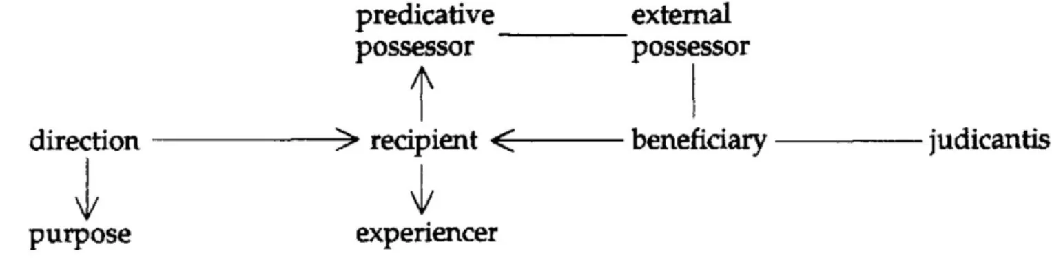
Figure 3. A semantic map of typical dative functions / the boundaries of English to
(based on Haspelmath 2003: 213, 215)
• ‘A semantic map is a geometrical representation of functions (…) that are linked by connecting lines and thus constitute a network’ (Haspelmath 2003).
Types of information
Figure 4. Dynamicized semantic map of dative functions (Haspelmath 2003: 234)
Le Diasema 13
Types of information
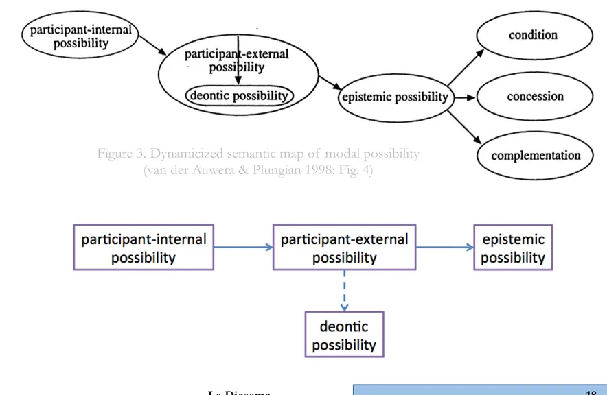
Figure 5. Dynamicized semantic map of modal possibility (van der Auwera & Plungian 1998: Fig. 4)
Types of information
Figure 6. Dynamicized semantic map of modal possibility (van der Auwera & Plungian 1998: Fig. 4)
Le Diasema 15
Types of information
Figure 7a. A simple semantic map of person marking(Cysouw 2007: 231)
Figure 7b. A weighted semantic map of person marking (Cysouw 2007: 233)
• Weighted semantic maps
Types of information
Le Diasema 17
Types of information
• Semantic relationships
Figure 5. Dynamicized semantic map of modal possibility (van der Auwera & Plungian 1998: Fig. 4)
ü DEONTIC POSSIBILITY (e.g., “as far as I’m concerned, you may go to the party tonight”) is defined as a subtype (hyponym) of PARTICIPANT–EXTERNAL POSSIBILITY
(e.g., “you may take the bus in front of the train station”)
ü PARTICIPANT–EXTERNAL POSSIBILITY and EPISTEMIC POSSIBILITY (e.g., “he may be at the office right now”) are seen as metonymically related
Types of information
• Semantic relationships
Figure 3. Dynamicized semantic map of modal possibility (van der Auwera & Plungian 1998: Fig. 4)
Le Diasema
19
Large-scale electronic resources
for lexical typology
Le Diasema 21
Electronic resources for lexical typology
Polysemy data from CLiCs (http://clics.lingpy.org/download.php)
Meaning 1 Meaning 2
N of language
N of
forms language:form
see know 5 6
aro_std:[ba]//ayo_std:[iˈmoʔ]//haw_std:[ʔike]//mcq_std: [ɓanahe]//mri_std:[kitea]//tel_std:[aarayu]//tel_std:[arayu]
see find 15 23 agr_std:[wainat]//arn_std:[pe]//con_std:[ˈatʰeye]//cwg_std: [yow]//emp_std:[uˈnu]//kgp_std:[we]//kpv_std:[addzɩnɩ]// kyh_std:[mah]//mca_std:[wen]//mri_std:[kitea]//oym_std:[ɛsa]// pbb_std:[uy]//plt_std:[mahìta]//pui_std:[duk]//ray_std:[tikeʔa]// rtm_std:[ræe]//sap_Enlhet:[neŋwetayˀ]//sei_std:[aʔo]//shb_std: [taa]//sja_std:[unu]//swh_std:[ona]//tbc_std:[le]//yag_std:[tiki] see get, obtain 6 6
kgp_std:[we]//mbc_std:[eraʔma]//pbb_std:[uy]//sap_Standard: [akwitayi]//srq_std:[tea]//udi_std:[акъсун] • N of lgs: 221 • N of lg families: 64 • N of concepts: 1280 (List et al. 2014)
Le Diasema 23
Le Diasema 25
Electronic resources for lexical typology
Electronic resources for lexical typology
Python script α Lexical matrix
Le Diasema 27
Electronic resources for lexical typology
Python script α Lexical matrix
Electronic resources for lexical typology
Python script α Lexical matrix
Languages Forms Meanings
Le Diasema 29
Electronic resources for lexical typology
Waiting for CLICS 2.0 … (List et al. 2018)
Electronic resources for lexical typology
Waiting for CLICS 2.0 … (List et al. 2018)
Increased quantity of data
1280 concepts => 2463 concepts (but ‘only’ 1521 colexified) 221 => 1156 language varieties (= 996 in Glottolog)
Le Diasema 31
Electronic resources for lexical typology
Waiting for CLICS 2.0 … (List et al. 2018)
Electronic resources for lexical typology
Waiting for CLICS 2.0 … Increased quality of data (e.g., links to the Concepticon) (List et al. 2018)
Le Diasema 33
Electronic resources for lexical typology
Waiting for CLICS 2.0 … Increased quality of data (e.g., links to the Concepticon)
Include partial colexifications
Normalize the data which is analysed by CLICS
(List et al. 2018)
Electronic resources for lexical typology
Synset: A synonym set; a set of words that are roughly synonymous in a given context
Core concept
Words are grouped together as sets of synonyms (Fellbaum 1998: 72ff.)
Le Diasema 35
Electronic resources for lexical typology
Synset: A synonym set; a set of words that are roughly synonymous in a given context
Core concept
Words are grouped together as sets of synonyms (Fellbaum 1998: 72ff.)
Le Diasema 37
Electronic resources for lexical typology
34 languages
OMW can be queried as a corpus with the Natural Language Tool-kit (NLTK)
interface in Python
Electronic resources for lexical typology
34 languages
OMW can be queried as a corpus with the Natural Language Tool-kit (NLTK)
interface in Python
Possible to build lexical matrix!
Method
1. Choose the basic senses belonging to the semantic field to be investigated (e.g., SEE, HEAR, LOOK, LISTEN)
2. Collect all the forms that lexicalize these 4 senses
3. Retrieve the list of all the senses of these forms (the total of the synsets in which this forms appear)
4. For each form, check whether the senses collected are among its senses
Le Diasema
39
Inferring classical semantic maps
from lexical matrices
Inferring semantic maps
“ideally (…) it should be possible to
generate semantic maps automatically
on the basis of a given set of data”
Le Diasema 41
Inferring semantic maps
Limitation of the semantic map method: practically impossible to
handle large-scale crosslinguistic datasets manually
“not mathematically well-defined or computationally tractable, making it impossible to use with large and
highly variable crosslinguistic datasets”
Inferring semantic maps
Limitation of the semantic map method: practically impossible to
handle large-scale crosslinguistic datasets manually
Figure 5. MDS analysis of
Regier, Khetarpal, and Majid showed that the semantic map inference
problem is “formally identical to another problem that superficially
appears unrelated: inferring a social network from outbreaks of disease
in a population”
(Regier et al., 2013: 91)
Le Diasema 43
• What’s the idea?
• Let’s consider a group of social agents (represented by the nodes of a potential graph)
• What’s the idea?
• If one observes the same disease for five of these agents (technically called a constraint on the nodes of the graph)
Le Diasema 45
• What’s the idea?
• One can postulate that all the agents met, so that all the nodes of the graph are connected (10 edges between the 5 nodes)
• What’s the idea?
• This is neither a very likely, nor a very economic explanation
Le Diasema 47
• What’s the idea?
• But this is precisely what a colexification network does
• What’s the idea?
• The goal would be to find a more economical solution and to have all the social agents connected with as few edges as possible
Le Diasema 49
• What’s the idea?
• Such a Network Inference problem looks intuitively simple, but is computationally hard to solve
• Cf. the travelling salesman problem [TSP]: “Given a list of cities and the distance between each pair of cities, what is the shortest possible route that visits each city exactly once?”
• Angluin et al. (2010) concluded that the problem is indeed computationally intractable, but proposed an algorithm that approximates the optimal
solution nearly as well as is theoretically possible
• How does it transfer to semantic maps?
Le Diasema 51
• How does it transfer to semantic maps?
• Nodes are meanings
Inferring semantic maps
Meaning 1
Meaning 5
• How does it transfer to semantic maps?
• Nodes are meanings
• Constraints are Polysemic items
Le Diasema 53
Inferring semantic maps
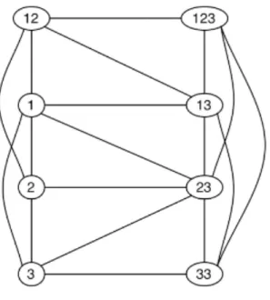
Meaning 1 Meaning 2 Meaning 5 Meaning 4 Meaning 3 Meaning 1 2 3 4 5 Polysemic item A √ √ Polysemic item B √ √ √ Polysemic item C √ √ √
• How does it transfer to semantic maps?
• Nodes are meanings
• Constraints are Polysemic items
• One connects the nodes economically based on these constraints
Inferring semantic maps
Meaning 1
Meaning 5
Meaning 1 2 3 4 5
• How does it transfer to semantic maps?
• Nodes are meanings
• Constraints are Polysemic items
• One connects the nodes economically based on these constraints
Le Diasema 55
Inferring semantic maps
Meaning 1 Meaning 2 Meaning 5 Meaning 4 Meaning 3 Meaning 1 2 3 4 5 Polysemic item A √ √
• How does it transfer to semantic maps?
• Nodes are meanings
• Constraints are Polysemic items
• One connects the nodes economically based on these constraints
Inferring semantic maps
Meaning 1
Meaning 5
Meaning 1 2 3 4 5
• How does it transfer to semantic maps?
• Nodes are meanings
• Constraints are Polysemic items
• One connects the nodes economically based on these constraints
Le Diasema 57
Inferring semantic maps
Meaning 1 Meaning 2 Meaning 5 Meaning 4 Meaning 3 Meaning 1 2 3 4 5 Polysemic item A √ √ Polysemic item B √ √ √ Polysemic item C √ √ √
• How does it transfer to semantic maps?
The result is a map that accounts for all the polysemy patterns, while remaining as economic as possible
Inferring semantic maps
Meaning 1
Meaning 5
Meaning 1 2 3 4 5
• Regier et al. (2013): the approximations produced by the Angluin et al. algorithm are of high quality
• Tested on the crosslinguistic data of Haspelmath (1997) and Levinson et al. (2003)
Le Diasema 59
Inferring semantic maps
Figure. Haspelmath’s (1997: 4) original semantic map of the indefinite pronouns functions
Inferring semantic maps
INPUT
Le Diasema 61
Inferring semantic maps
INPUT
(lexical matrix)
ALGORITHM
Inferring semantic maps
INPUT
(lexical matrix)
ALGORITHM
• Weighted semantic maps are much more informative than regular semantic
maps, because they visually provide information about the frequency of
polysemy patterns
• Diachronic semantic maps are much more informative than regular
semantic maps, because they visually provide information about possible
pathways of change
Le Diasema 63
Automatic plotting: Two steps forward
“[T]he best synchronic semantic map is a diachronic one”
• Generate the map with a modified version of the algorithm of
Regier et al. (2013)
• PRINCIPLE: for each edge that is being added between two meanings
of the map by the algorithm, check in the lexical matrix how many times this specific polysemy pattern is attested, and increase the weight of the edge accordingly
Automatic plotting: Two steps forward
Weighted semantic maps
• Generate the map with a modified version of the algorithm of
Regier et al. (2013)
• PRINCIPLE: for each edge that is being added between two meanings
of the map by the algorithm, check in the lexical matrix how many times this specific polysemy pattern is attested, and increase the weight of the edge accordingly
• Based on the data of Haspelmath (1997), kindly provided by the author, the result between a non-weighted and a weighted semantic map are markedly different
Le Diasema 65
Automatic plotting: Two steps forward
Weighted semantic maps
Automatic plotting: Two steps forward
Weighted semantic maps
Automatically plotted semantic maps: non-weighted vs. weighted (data from Haspelmath 1997)
Le Diasema 67
Automatic plotting: Two steps forward
Weighted semantic maps
Automatically plotted semantic maps: non-weighted vs. weighted (data from Haspelmath 1997)
The graph is visualized in Gephi® with the Force Atlas algorithm and modularity analysis (Lambiotte et al. 2009)
• Expand the lexical matrix so as to include information about diachrony
Automatic plotting: Two steps forward
Diachronic semantic maps
• Expand the lexical matrix so as to include information about diachrony
Le Diasema 69
Automatic plotting: Two steps forward
Diachronic semantic maps
The diachronic stages are arbitrarily indexed by numbers:
• Expand the lexical matrix so as to include information about diachrony
Automatic plotting: Two steps forward
Diachronic semantic maps
• Generate the graph with the algorithm of Regier et al. (2013)
Le Diasema 71
Automatic plotting: Two steps forward
Diachronic semantic maps
• Generate the graph with the algorithm of Regier et al. (2013)
• Enrich the graph with oriented edges (where relevant)
• PRINCIPLE: (1) we convert the undirected graph into a directed graph
(2) for each edge in the graph, if the meaning of node A is attested for one diachronic stage, while the meaning of node B is
not, check in the lexical matrix if there is a later diachronic stage of the same language for which this specific word has both meaning A and B (or just meaning B). If this is the case, we can
infer a meaning extension from A to B.
Automatic plotting: Two steps forward
Diachronic semantic maps
Le Diasema 73
Automatic plotting: Two steps forward
Diachronic semantic maps
INPUT (diachronic lexical matrix)
Automatic plotting: Two steps forward
Diachronic semantic maps
INPUT (diachronic lexical matrix) ALGORITHM (python script for inferring oriented edges)
Le Diasema 75
Automatic plotting: Two steps forward
Diachronic semantic maps
INPUT (diachronic lexical matrix) ALGORITHM (python script for inferring oriented edges) RESULT (dynamic semantic map)
Exploring automatically-plotted
semantic maps
Le Diasema 77
Le Diasema 79
Layout, weights, modularity
TIME-RELATED MEANINGS
Layout, weights, modularity
TIME-RELATED MEANINGS
Le Diasema 81
Layout, weights, modularity
TIME-RELATED MEANINGS
Layout, weights, modularity
TIME-RELATED MEANINGS
Le Diasema 83
Layout, weights, modularity
TIME-RELATED MEANINGS
Layout, weights, modularity
TIME-RELATED MEANINGS
Le Diasema 85
Layout, weights, modularity
TIME-RELATED MEANINGS
Layout, weights, modularity
TIME-RELATED MEANINGS
Le Diasema 87
Layout, weights, modularity
TIME-RELATED MEANINGS
Layout, weights, modularity
TIME-RELATED MEANINGS
Le Diasema 89
Layout, weights, modularity
ü Easy to read
ü Generates interesting hypotheses and avenues for research in lexical typology
BUT
u The mapping of forms is hard to achieve;
cf. Cysouw (2007) ‘it overgenerates
constellations of meaning’ u Hence, one cannot tell
which patterns are precisely attested
Le Diasema 91
Methodological issues
Methodological issues
• Hill & List (2017): Bipartite networks
“Bipartite networks are networks consisting
of two types of nodes. Edges in these
networks are only allowed to be drawn from
nodes of one type to nodes of another type.
In our case the first node type are the
concepts in the concept list and the second
node type are the word forms in a given
language. We create our network by linking
all individual morphemes in our data to the
Le Diasema 93
Methodological issues
• Hill & List (2017): Bipartite networks
• List et al. (2018): Hypergraph
Methodological issues
• Hill & List (2017): Bipartite networks
• List et al. (2018): Hypergraph
How can we visualize the types of polysemy patterns attested
Werning (2012)
Le Diasema 97
Methodological issues
• Hill & List (2017): Bipartite networks
• List et al. (2018): Hypergraph
• Ryzhova & Obiedkov (2017): Formal concept analysis
Methodological issues
FCA solves the problem of form/ meaning mapping, since it shows: ü How forms maps onto
meanings
ü Which concepts are lexicalized and which are not
ü Implication sets can be computed automatically
Le Diasema 99
Methodological issues
Figure 3. FCA analysis of Haspelmath’s (1997) data
FCA solves the problem of form/ meaning mapping, since it shows: ü How forms maps onto
Methodological issues
FCA solves the problem of form/ meaning mapping, since it shows: ü How forms maps onto
meanings
ü Which concepts are lexicalized and which are not
Le Diasema 101
Methodological issues
Figure 3. FCA analysis of Haspelmath’s (1997) data
FCA solves the problem of form/ meaning mapping, since it shows: ü How forms maps onto
meanings
ü Which concepts are lexicalized and which are not
Methodological issues
FCA solves the problem of form/ meaning mapping, since it shows: ü How forms maps onto
meanings
ü Which concepts are lexicalized and which are not
ü (Implication sets can be computed automatically)
Le Diasema 103
Methodological issues
1.
How can we visualize the types of polysemy patterns attested?
2.
How can we deal with studies that take a single meaning as point
Le Diasema 105
Le Diasema 107
Le Diasema 109
Le Diasema
111