Modelica Library
Q. Altés Bucha, R. Dickesa, A. Desideria, V. Lemorta and S. Quoilina*
a
Energy Systems Research Unit, Université de Liège, Campus du Sart-Tilman, B-49, Liège, Belgium *
squoilin@ulg.ac.be Abstract:
This paper proposes an innovative approach for the dynamic modeling of heat exchangers without phase transitions. The proposed thermo-flow model is an alternative to the traditional 1D finite-volumes approach and relies on a lumped thermal mass approach to model transient responses. The heat transfer is modeled by the well-known Logarithmic Mean Temperature Difference approach, which is modified to ensure robustness during all possible transient conditions. The lumped parameter models are validated with references models and tested within a Concentrating Solar Power plant model. Results indicate that the developed lumped models are robust and computationally efficient, ensuring the convergence of the Newton Solver. They are significantly faster (~10-fold) than the traditional finite volume models, although a more extensive comparisons would be needed to confirm this figure. They are well suited to be integrated in larger system models, but are not appropriate for the simulation of detailed thermo-flow phenomena.
Keywords:
CSP, Dynamic modeling, Lumped parameter, Modelica, Semi-empirical, Steam cycle, ThermoCycle.
1. Introduction
Dynamic simulation of thermodynamic systems is required to evaluate and optimize their response time, or to define, implement and test control strategies. The Modelica language is well adapted to the formulation of thermo-flow problems, mainly because it is an a-causal language that allows interconnecting the models in a "physical" way [1]. In recent years, several libraries have been developed to model thermodynamic and thermal systems in Modelica. A number of tools are now available to model steam and gas cycles (e.g. ThermoSysPro, Power Plants, Thermal Power, ThermoPower, etc.) or refrigeration systems (TIL, AirConditioning, etc.).
Most of these libraries and simulation tools rely on finite volume approaches for thermo-flow problem (e.g. ThermoPower [2], ThermoCycle [3], TIL [4]). They propose detailed models, in which the accurate geometry of each component must be user-defined. Heat exchangers are usually discretized, which involves many thermodynamic property calls and multiplies the number of nonlinear equations (at least one per cell or node). Therefore, these models are subject to lack of robustness (i.e. the convergence of the Newton Solver is not ensured) and are computationally-intensive [5].
Discretized heat exchanger models can be advantageously replaced by lumped dynamic models based on the epsilon-NTU or LMTD methods [6]. Such an approach is appropriate for the following cases:
▪ The level of detail required by the model is low. Its main goal is the evaluation of the component behavior integrated in a wider system, rather than the accurate computation of, e.g, the heat transfer and pressure drop. This is especially the case when implementing and testing control strategies of a whole system or power plant.
▪ The heat exchanger exact geometry is unknown. In this case, a simplified lumped approach is more appropriate than a detailed model, provided that the main physical phenomena are taken into account.
In this work, a simplified but still physically meaningful, semi-empirical heat exchanger dynamic model is proposed and included into the open-source ThermoCycle Modelica Library [3]. The models are based on a lumped approach, which allows for robustness and computational efficiency. The proposed models are compared in terms of robustness and simulation speed to the traditional finite volume heat exchanger model present in the ThermoCycle library. A detailed model of a 2-MW steam power plant coupled to concentrated solar power (CSP) is then developed based on the proposed heat exchanger lumped model, for the purpose of evaluating the system’s reaction to transient conditions. The proposed model proved to be more robust and significantly faster than traditional models.
2. Proposed simplified models
In this work a simplified lumped-parameter heat exchanger model is presented, based on a modified version of the LMTD method. This method was originally developed for steady-state simulation. The proposed method called robust LMTD (RLMTD), is developed to handle the crossing of the temperature profiles (negative pinch point) making it suitable for dynamic modeling.
The model has been developed for single-phase (i.e., economizer, super-heaters) operation only and it is intended to be very simple, in order to maximize the robustness and the simulation speed, while maintaining an acceptable accuracy. It is based on a static energy and mass balance on the two fluid sides and thermal energy accumulation in the metal wall. The thermal masses of the two fluids and of the wall are lumped into a single thermal mass situated in the wall. Contrary to a steady-state model, the heat transfer problem is divided in two:
▪ A first heat transfer between the hot fluid and the wall
▪ A second heat transfer between the wall and the cold fluid
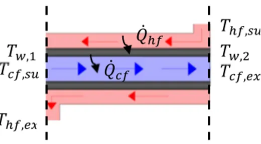
Fig. 1. Sketch of the variables used in the model
No temperature gradient is considered through the wall thickness. The two computed heat flows are not necessarily equal, the difference between them corresponding to the thermal energy accumulation or rejection of the metal wall (see Fig. 1), which is accounted for by (1):
(1) where is the mass of the wall, is the specific heat capacity of the wall, is the mean temperature in the wall, and and are the heat power transferred by the hot fluid and received by the cold fluid respectively. The above equation allows computing the average wall temperature, but not the temperature gradient within the wall. In the absence of axial conduction in the wall, the evolutions of the temperatures in two infinitely small volumes at each extremity of the heat exchanger are given by (2) and (3):
, ∆ , ∙ , , , , (2)
, , ,
, ∆ , ∙ , , , , (3)
where the subscript “1” and “2” indicate both extremities of the heat exchanger.
In a first approximation, the temperature evolutions can be considered linear with the axial distance and the two previous equations can be integrated from 1 to 2, leading to (4):
∆
, , ∆ , , ∆ (4)
where ∆ is the temperature gradient within the wall.
Equation (4) provides the slope of the temperature profile, and (1) provides its average value. This temperature is therefore entirely defined by these two equations.
It is important to underline that no mass accumulation is considered in the model. Therefore, the outlet flow rate is always equal to the inlet flow rate for both sides of the heat exchanger.
2.1. Robust LMTD Method
The heat exchanger model comprises three different temperature profiles: the secondary fluid, the wall and the working fluid. As previously mentioned, the goal is to compute the two heat flows using the LMTD method, which is applied twice: between the secondary fluid and the wall, and between the wall and the working fluid temperature profiles.
However, in dynamic simulation, temperature profiles can cross each other for a period of time, a condition that impedes the use of the traditional LMTD method. Furthermore during the initialization process, temperature profiles are highly variable, which can also lead to simulation failures in case of crossing.
In [7],a formalism was set up to avoid numerical failures during the iterations of the Newton solver (i.e. for steady-state simulation only). The idea behind this method is to rewrite the heat transfer model using causal equations only, instead of leaving the iterative process to the solver. This method presents the advantage of allowing conditional statement and therefore brings a solution if negative pinch points appear during the iterations, by modifying the LMTD equation to avoid logarithms of negative numbers.
This method has been reformulated for dynamic simulation and extended to ensure smoothness. The result is the robust LMTD function reported in (5) to (9).
∆ !"#$ ∆ ∆ ln'∆ ( ln '∆ ( if ∆ ) *, ∆ ) * and ∆ + ∆ (5) ∆ ∆ 2 if ∆ ) *, ∆ ) * and ∆ ∆ (6) ∆ * ln -∆#. / 0 '1 2 '∆ *(( if ∆ ) * and ∆ 3 * (7) ∆ * ln -∆#4 / 0 '1 2 '∆ *(( if ∆ 3 * and ∆ ) * (8) * 1 2 '∆ *( '1 2 '∆ *(( if ∆ 3 * and ∆ 3 * (9)
where * and 2 are two parameters to set by the user whose influence is described below.
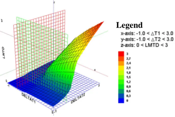
An isometric view of a 3-D representation of the RLMTD function for a range of temperature gradients between the working or secondary fluid and the wall is shown in Fig. 2. Temperature
differences on the two sides of the heat exchanger vary from minus one to three Kelvin. The position of the grids corresponds to DELTAT=0.
Fig. 2. 3-D plot of the RLMTD function
An important feature of this function is that it is C0-continuous, which allows an easier convergence of the solver. Nonetheless, it can be seen in Fig. 3 that the derivatives of the function are not continuous. A modification of the RLMTD function with splines functions could therefore be implemented to make it C1-continuous, which could further increase the computational efficiency of the heat exchanger model. As shown in Fig. 2, RLMTD depends on the two temperature differences and is non-null when ∆T = 0. In this manner, the function is computable even for negative temperature gradients. This avoids simulation failure, e.g. in case of temperatures profile crossing. However, it must be noticed that a positive LMTD value when pinch points are negative lead to a non-physical behavior: the heat flow remains positive (although very small), even for negative temperature differences, i.e. the heat flow is being transferred from the cold to the hot side.
Therefore, LMTD value for negative pinches should be as small as possible so that the leakage heat flow can be neglected. Parameters * and 2 play a key role at this point:
▪ ξ influences how fast LMTD goes to zero, as shown in Fig. 4 and 6. Small ξ values lead to
higher LMTD values at ∆T = 0, and thus to higher leakage heat flow. On the other hand, high ξ values entail steep variations of the RLMTD function, which can also lead to simulation failures.
▪ ε is the threshold (in terms of DELTAT value) below which the LMTD function is replaced by a
decreasing polynomial function (see equations (5) to (9)). It should therefore be set to a lower value than the nominal pinch points of the modeled heat exchangers in order to ensure the validity of the LMTD method in usual operating conditions. As for ξ, it should however not be too small to avoid slow and non-robust simulation (Fig. 4 and 5).
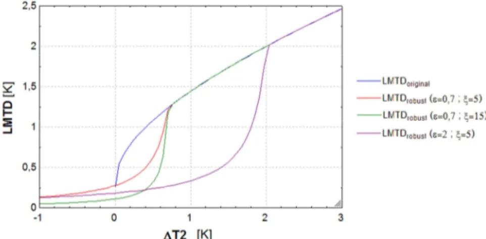
Fig. is a comparison of the RLMTD when varying the parameters * and 2, for the range of temperature gradient ∆T2 ∈ ' 1 , 3( and holding ∆T1 at the constant value of 2 K. The original LMTD method has also been plotted.
Fig. 3. Plot of three different LMTD robust function and original LMTD function
Fig. 4 to Fig. 6 present three 3-D surface of the RLMTD function, with different values for the parameters. LMTD original function has also been plotted in Fig. 7.
Fig. 4. 0.7 ; 2 5 Fig. 5. * 2 ; 2 5
Fig. 6. * 0.7 ; 2 15 Fig. 7. LMTD original
3. Model validation
The developed lumped model is compared to the discretized counter-current heat exchanger from the ThermoCycle library. The main goal is to verify that the lumped heat exchanger model presents a dynamic behavior similar to that of the discretized one. The comparison is carried out by analyzing the models when subjected to the same transient condition:
▪ Temperature step (hot fluid)
▪ Mass-flow rate step (cold fluid)
The robustness and computational efficiency of both models, which are the main focus of this work, will be also evaluated and compared.
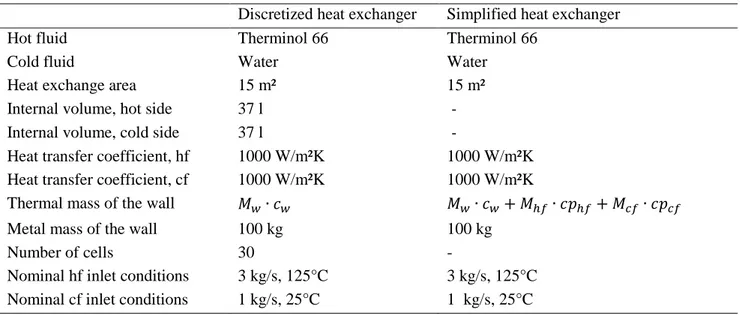
As above mentioned, in the simplified heat exchanger, the thermal masses of the fluid are lumped into the thermal mass of the wall, as shown in Table 1.
↑;
↑<
Legend Legend
Table 1. Heat exchanger parameters for the comparison Discretized heat exchanger Simplified heat exchanger
Hot fluid Therminol 66 Therminol 66
Cold fluid Water Water
Heat exchange area 15 m² 15 m²
Internal volume, hot side 37 l
-Internal volume, cold side 37 l
-Heat transfer coefficient, hf 1000 W/m²K 1000 W/m²K Heat transfer coefficient, cf 1000 W/m²K 1000 W/m²K
Thermal mass of the wall ∙ ∙ ∙ = ∙ =
Metal mass of the wall 100 kg 100 kg
Number of cells 30 -
Nominal hf inlet conditions 3 kg/s, 125°C 3 kg/s, 125°C Nominal cf inlet conditions 1 kg/s, 25°C 1 kg/s, 25°C
3.1. Response to steps
3.1.1. Temperature step on hot fluid
The first simulation consists in applying a step of 150K on the inlet temperature of the hot fluid. The simulation of this step with the two heat exchanger models leads to a good agreement between the outlet temperature profiles of each side, as shown in Fig. 8. A small discrepancy is only visible directly after the step: the simplified model does not reproduce the small response delay visible with the discretized heat exchanger. This delay is due to the temperature front propagation within the heat exchanger, which is no taken into account in the simplified model. Results also show that the dynamics is well reproduced for the cold fluid (i.e. on the other side of the step), but with a slightly higher difference for the outlet temperature of the side where the step is applied.
3.1.2. Mass-flow rate step on cold fluid
In this simulation a step is applied on the mass flow rate of the cold fluid, keeping the inlet temperatures constant. The results are presented in Fig. 9 and with a good agreement between both models.
Fig. 8. Simulation results when applying a temperature step on the hot fluid
Fig. 9. Simulation results when applying a step on the mass-flow rate on the cold fluid
3.2. Simulation speed
In order to assess the computational efficiency of the model, a comparison of the simulation speed of each model is performed for the two simulations presented above: step on inlet temperature of hot fluid and step on the mass flow rate of the cold fluid. The comparison is performed on the basis of the CPU time for integration with a 1000s simulation.
Table 2. Simulation time for integration
Heat exchanger Simulation Step Time [s]
Discretized Temperature (hot fluid) 26
Mass flow rate (cold fluid) 21.6
Simplified Temperature (hot fluid) 2.3
Mass flow rate (cold fluid) 2.64
Table 2 shows that a significant increase in computational efficiency can be obtained with the lumped model: it is about 11 times faster than the finite volume model for a temperature step and about 8 times faster for a step on the mass flow rate.
4. Real test case
A dynamic model of a real cycle has been built for the purpose of evaluating the suitability of the proposed models for larger system simulations. In order to provide realistic parameters, the models have been tested for the modeling of a 2-MW parabolic through CSP system coupled to a Rankine cycle power plant. The parameters of the steam power plant correspond to those of an extraction-condensing CHP plant connected to a district heating network of the University campus in Liège (Belgium).
4.1. Overall system model
After the development of each subcomponent model, a dynamic model of the overall cycle is built. The model consists in a steam cycle coupled to a parabolic troughs model.
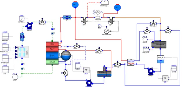
Fig.10. Diagram of the cycle used for the simulations
For the steam cycle, two turbines are connected in series to allow modelling turbine bleeding and regeneration. After them, the fluid flows through the condenser, being its main entrance. Because the developed cross-condenser in [8] does not consider the condensed steam flow collected at the bottom of the condenser, a liquid receiver model from the ThermoCycle library is added in series,
which allows computing the working pressure of the condenser. The main feed pump extracts the condensed steam and circulates it to the preheater, where it is heated up while receiving heat from a portion of super-heated steam extracted before the high pressure turbine. The feed water from the preheater is then sent to the deaerator, which is meant to remove non-condensable gases due to the low working pressure. The water stored in the deaerator vessel is then pumped to the boiler system by the feed pump.
The heat transfer fluid coming from the parabolic troughs field enters at its maximum temperature in the superheaters, then flows through the evaporator and finally through the economizer, before being returned to the collectors to be heated up again.
4.2. Boiler system
The boiler layout is presented in Fig. 11 with the main system subcomponents, i.e. an economizer, an evaporator, two superheaters, a pump, two pressure drops and a drum.
Fig.11. Sketch of the boiler system Fig.12. Boiler system subcomponents
All heat exchangers in the boiler are modeled with the lumped model proposed in this work. For the evaporator (i.e. with a two-phase side), the model has been slightly modified to allow computing the LMTD in semi-isothermal conditions [8]. Since the heat exchanger model does not take into account the pressure drop, a separate model is inserted in series for that purpose, as shown in Fig. 12.
The liquid flow rate exiting the drum is imposed by the evaporator pump, whose speed is set in regard to the outlet vapor quality in the evaporator. The vapor outflow of the drum mainly flows to the superheater section, although a little fraction is used for the deaerator (represented by an outflow connector). The super-heater section is divided in two super-heaters, with a possibility to perform de-superheating which is not modeled in this work. This allows controling the temperature of the vapor entering the high pressure turbine.
4.3. Example of simulation: Varying the DNI
The main purpose of this simulation is to see the dynamic reaction of the system to a variation of the ambient conditions, and to validate the use of lumped heat exchanger models for such a simulation. The simulation consists in submitting the cycle into transient conditions such as varying the solar irradiation data. The irradiation, input of the solar filed model, has been defined as a step that varies from 1000 W/m2 to 500 W/m2 after steady-state conditions are achieved for all variables.
Following this step variation, the temperature at the outlet of the collectors decreases from approximately 385ºC to 275ºC. The output power is reduced from 2,2MW to 1MW. It should be noted that no control system has been implemented in this simulation, the main focus being the response of the different components to varying boundary conditions, and the response delays in different parts of the cycle, such as the superheating temperature, the pressure in the boiler, the electrical power produced by the turbines and the condensing pressure. In order to compare the
magnitude of these delays, all variables have been normalized (i.e., their values move between 0 and 1), and plotted in Fig. 13.
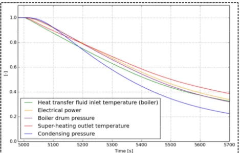
Fig. 13. Response to key cycle values to a step. All values have been made non-dimensional, varying between 1 and 0
Fig. 14. Zoom of Fig. 13
Fig. 14 shows a small delay in the response of all variables after the step (t=5000s). The delays are different depending on the type and the situation of the considered variable. As shown in Fig. 14, just after the step (5000 to 5100s), the reaction time of the different variables are ordered in the following manner (from the fastest to the slowest): (1st) boiler secondary fluid (HTF) inlet temperature, (2nd) super-heating outlet temperature, (3rd) electrical power, (4th) boiler drum pressure and (5th) condensing pressure.
However, after a certain simulation time (5500 to 5700s), this order is modified and becomes: (1st) condensing pressure, (2nd) boiler drum pressure, (3rd) electrical power, (4th) boiler secondary fluid (HTF) inlet temperature and (5th) super-heating outlet temperature.
This phenomenon can be explained in the following way: just after the step (t=5000s), the response time of the different variables is explained by a “proximity parameter”. The heat transferred to the oil decreases, so the temperature at the outlet of the collectors (i.e. boiler secondary fluid inlet temperature) is the first affected variable. The following effects are in the boiler. The super-heating outlet temperature is the second affected, because it depends on the inlet temperature of the oil in the boiler. The boiler’s drum pressure, will also decrease, and with it, the boiler mass flow rate. With a lower super-heating temperature of the fluid flowing through the turbines and a lower flow rate, the electrical power produced becomes smaller. Finally, the fluid exiting the turbines with a lower flow rate will affect the condensing pressure.
After a certain simulation time, the “proximity” effect becomes irrelevant, and the response time mainly depends on the “natural” dynamics of the system. The pressure in the condenser, for example, is largely independent of the rest of the cycle, which explains why it is the fastest to decrease to its new steady-state value. On the contrary, the temperature of the oil, which was obviously the first effect of varying the solar irradiation data, continues changing in a slower pace. The boiler’s pressure and the electrical power remain closely related one to another, i.e. as soon as the first one decreases (leading to a lower flow rate), the second one follows it.
5. Conclusions
The main goal of this work was to design a library of semi-empirical dynamic models that are simplified but also physically meaningful, and whose main characteristics are robustness, ease of parameterization and computational efficiency.
The selected approach to achieve the above objectives was to simplify the different component models to get rid of non-essential effects for the purpose of the simulation.
The main characteristic of the library is the LMTD formulation for the heat exchanger models. This formulation, which is originally only valid for steady-state, has been extended to transient simulation by dividing the heat transfer problem in two and adding a lumped thermal mass. The single-phase heat transfer function RLMTD significantly increases the robustness of the model. The model does not take into account heterogeneous flow (i.e. a slip factor between the vapor and liquid phases) or mass accumulation within the heat exchanger.
The proposed models have been validated by comparison with a reference well-known 1D finite-volumes model. The response to step variations of the boundary conditions agree remarkably, except if the very fast transients after the disturbance are considered. Simulation time is decrease by a factor close to 10 with the lumped model.
The robustness and the ability of the proposed model to be integrated into a larger system have then been tested using the case of a CSP plant coupled to a steam cycle. All heat exchangers of the steam boilers have been successfully replaced by the proposed ones. The overall simulation proved to be both robust and computationally efficient, which were the main goals of this work
Future works will focus on the formulation of recommendations regarding the use of such models (i.e. criteria to ensure acceptable accuracy, parameterization guidelines, limitations…). In addition, the simulation of the overall system presented here should be compared to experimental data and/or to a reference previously validated model.
It is finally worthwhile to note that all the models presented here have been made available in an open-source format within the ThermoCycle library and can be freely re-used and adapted.
Acknowledgements
The results presented in this paper have been obtained within the frame of the IWT SBO-110006 Project “The Next Generation Organic Rankine Cycles”, funded by the Institute for the Promotion and Innovation by Science and Technology in Flanders (IWT). This financial support is gratefully acknowledged.
Nomenclature
AU heat transfer conductance, W/K
> specific heat capacity, J/kgK
M mass, kg
Q heat power, W T temperature, ºC or K
x vapor quality, –
Greek symbols
∆ differential
ε parameter or RLMTD, –
ξ penalty factor, –
Subscripts and superscripts
cf cold fluid eco economizer eva evaporator ex exhaust hf hot fluid sf secondary fluid sh1 first superheater sh2 second superheater su supply w wall wf working fluid Acronyms
CHP Combined Heat and Power CSP Concentrated Solar Power DNI Direct Normal Irradiation HTF Heat Transfer Fluid
LMTD Log Mean Temperature Difference
References
[1] Casella F., van Putten J.G., Colonna P., Dynamic simulation of a biomass-fired steam power plant: a comparison between causal and a-causal modular modeling. In: ASME 2007 International Mechanical Engineering Congress and Exposition, (American Society of Mechanical Engineers); 2007; pp. 205–216.
[2] Casella F., Leva A., Modelling of thermo-hydraulic power generation processes using Modelica. Taylor & Francis Online 2006.
[3] Quoilin S., Desideri A., Wronski J., Bell I., Lemort V, ThermoCycle: A Modelica library for the simulation of thermodynamic systems. In: 10th International Modelica Conference; 2014. [4] Gräber M., Kosowski K., Richter C., Tegethoff W., Modelling of heat pumps with an
object-oriented model library for thermodynamic systems. Taylor & Francis Online 2010.
[5] Quoilin S., Bell I., Desideri A., Dewallef P., Lemort V., Methods to increase the robustness of finite-volume flow models in thermodynamic systems. Energies 7, 2014; 1621–1640.
[6] Bell I., Quoilin S., Georges E.; Braun J.E., Groll E.A., Horton W.T., Lemort V., A Generalized Moving-Boundary Algorithm to Predict the Heat Transfer Rate of Counterflow Heat Exchangers for any Phase Configuration, Applied Thermal Engineering, 2015; in press.
[7] Quoilin S., Sustainable Energy Conversion Through the Use of Organic Rankine Cycles for Waste Heat Recovery and Solar Applications. Liège, Belgium: University of Liège; 2011. [8] Altés Buch Q., Dynamic modeling of a steam Rankine cycle for concentrated solar power