HAL Id: hal-00975237
https://hal-ensta-paris.archives-ouvertes.fr//hal-00975237
Submitted on 8 Apr 2014
HAL is a multi-disciplinary open access
archive for the deposit and dissemination of sci-entific research documents, whether they are pub-lished or not. The documents may come from teaching and research institutions in France or abroad, or from public or private research centers.
L’archive ouverte pluridisciplinaire HAL, est destinée au dépôt et à la diffusion de documents scientifiques de niveau recherche, publiés ou non, émanant des établissements d’enseignement et de recherche français ou étrangers, des laboratoires publics ou privés.
Wind Turbine Noise Modelling Based on Amiet’s Theory
Yuan Tian, Benjamin Cotté, Antoine Chaigne
To cite this version:
Yuan Tian, Benjamin Cotté, Antoine Chaigne. Wind Turbine Noise Modelling Based on Amiet’s Theory. 5th International Meeting on Wind Turbine Noise, Aug 2013, Denver, CO, United States. CD-ROM proceedings. �hal-00975237�
1
5th International Meeting
on
Wind Turbine Noise
Denver 28
– 30 August 2013
Wind Turbine Noise Modelling Based on Amiet's Theory
Y.Tian ENSTA ParisTech, 828, boulevard des Maréchaux, 91762 Palaiseau
Cedex, France
[email protected]
B. Cotté
[email protected]
A. Chaigne
[email protected]
Summary
Broadband noise generated aerodynamically is the dominant noise source for a modern wind turbine(Brooks et al, 1989; Oerlemans et al, 2007). In this paper, two main broadband noise mechanisms, namely trailing edge noise and turbulent inflow noise, are examined in detail using frequency domain noise prediction models based on Amiet's analytical theory. Improvements are proposed to adapt the original model to wind turbines . First, a wall pressure spectral model proposed recently by Rozenberg, Robert and Moreau that considers an adverse pressure gradient flow (APG) is applied to the trailing edge noise model. This APG model leads to a significant increase in the sound pressure level. Second, an empirical airfoil thickness correction is proposed in the turbulent inflow noise model, which introduces a level reduction that depends on leading-edge thickness, frequency and the ratio of the turbulence integral length scale to the blade chord. The proposed model also includes Doppler effect for rotating blades. Calculation results are validated by comparison with wind tunnel experimental data and with measurements for a full size wind turbine. This model is also used to quantify the amplitude modulation that can be a source of annoyance in the vicinity of a wind farm.
1. Introduction
Nowadays, wind energy application grows rapidly as a renewable, clean energy. While profiting from wind energy, the noise produced by a modern wind turbine becomes a main problem for the neighbourhood of a wind farm. The annoyance due to amplitude modulation (swish) and to the low frequency noise is especially a concern for the people living close to a wind farm (Styles et al, 2011).
Two main noise sources from modern wind turbines are turbulent inflow noise and trailing edge noise (Oerlemans et al, 2007). The former is induced by the scattering of atmospheric turbulence fluctuation at the leading edge of the blade, sometimes referred to as the leading edge noise; the latter is due to the turbulent boundary layer passing by a sharp edge like the trailing edge. Both noise mechanisms are broadband, and depend on the wind turbine size and on the atmospheric turbulence conditions; the total noise level can be dominated by one or the other.
The goal of this paper is to propose a theoretical noise prediction model, that can be used to study different phenomena related to wind turbine noise (amplitude modulation, wind shear effects, etc). The model is also intended to be coupled to an atmospheric propagation model for the prediction of the far field sound pressure level (SPL). In this paper, a well known analytical model proposed by Amiet (1975,1976) is chosen for the noise prediction. The original model is based on a flat plate with semi-infinite chord. As an improvement, an empirical correction on airfoil thickness for turbulent inflow noise is applied. Results show that increasing airfoil reduces the turbulent inflow noise. Furthermore, a wall pressure spectra model proposed by Rozenberg
et al. (2012), which considers an adverse pressure gradient (APG) flow is validated and applied
2
level to a certain level that depends on the flow conditions. The paper is organized as follows: in section 2, a brief introduction to the Amiet's analytical model is given; in section 3, two main improvements, namely, airfoil leading edge thickness and the APG model for the trailing edge noise are explained in detail; section 4 shows the validation for the improved models against the measurements of fixed airfoils; section 5 contains the results from a real size wind turbine calculation validated against the measurements; the conclusions and acknowledgements are in section 6.
2. Amiet's Analytical model for turbulent inflow noise and trailing edge
noise
In this section, Amiet's analytical models for both noise mechanisms are briefly introduced. Section 2.1 is devoted to turbulent inflow noise and section 2.2 to trailing edge noise.
2.1. Amiet's model for turbulent inflow noise
An airfoil in a turbulent flow experiences a fluctuation lift loading (unsteady upwash) which will result in the generation of sound. Considering the complex nature of turbulence and its interaction with the airfoil, many previous researchers proposed their models based on some common assumptions (Howe, 1978): 1. the incoming turbulence fluctuation is considered to be small compared to the mean flow velocity; 2. the interaction between an airfoil and the turbulent flow is inviscid so that the problem is reduced to solving linearized Euler equations. In Amiet's model (Amiet, 1975), the turbulent gust properties are assumed unchanged while it is convected by the mean flow, and its velocity fluctuation is represented in terms of chord-wise and span-wise wave number, here, and respectively, (see Figure 1). The airfoil is modelled as a flat plate with no thickness, where the chord is and the span is . The model further assumes that the plate has semi-infinite chord and infinite span extension.
Fig.1 Geometry and notations used in the turbulent inflow noise model.
If we write the incident gust in the Fourier domain in the form as:
, (1)
then the fluctuating velocity field is deduced as:
(2)
where is the velocity potential and is the Mach number, . Substituting Equation (2) into the convective wave equation we obtain:
̅
̅
̅
where
̅ ̅ ̅ ̅ ̅ ̅ is half chord, is the acoustic wave number, and
̅ ̅ ̅ ̅ ̅
with the free stream velocity. Solving for and using the relationship between acoustic pressure and velocity potential, we can finally get the pressure fluctuating on the airfoil surface as (Rozenberg, 2007):
3 √ ̅ , (3) with .
Assuming that the source behaves like a dipole source, and applying Lighthill analogy, the power spectrum density of far field acoustic pressure is obtained from Equation (3) as (Amiet, 1975; Rozenberg 2007):
⃗ ∫
[
] (4)
where is the air density, and is the sound velocity. ⃗ is the observer coordinate, is the airfoil response function, , is a modified distance between the source and observer. is the turbulence energy spectrum. If we assume a infinite span, , the function could be evaluated by a Dirac function, and thus Equation (4) reduces to:
⃗ (5)
Equation (5) is referred to as the simplified equation under large aspect ratio assumption.
2.2 Amiet's model for trailing edge noise
Trailing edge noise is generated by the scattering of the turbulent boundary layer passing by the trailing edge. Since the origin is the fluctuation of turbulent boundary layer, the derivation is similar to that of turbulent inflow noise, here only the final result, the power spectrum density of far field sound is cited as (Amiet, 1976; Roger et al. 2005):
⃗ ∫
[
] (6) ⃗ (7)
which are the exact formula and simplified formula under large aspect ratio assumption respectively. is the power spectral density of wall pressure, and is the span-wise correlation length.
3. Model improvement: adverse pressure gradient wall pressure model and
leading edge thickness correction
3.1 Airfoil thickness correction for turbulent inflow noise
Roger and Moreau (2010) studied the influence of airfoil leading edge thickness on far field sound pressure level. They show that an increase of leading edge thickness leads to the reduction of turbulent inflow noise. We propose here an empirical correction based on the data shown in Figure 6 of their publication. The reduction level in dB is calculated by linear interpolation based on the these data:
(8)
where is the airfoil maximum thickness, and is the turbulent integral length scale. The subscription stands for the value of reference experimental data, which is:
and .
3.2 Adverse pressure gradient wall pressure model for trailing edge noise
In Amiet's trailing edge noise model, one of the most important input parameters is the spectrum of fluctuating wall pressure. An accurate estimation of this spectrum can be done with
4
direct numerical simulation (DNS) or large eddy simulation (LES), but it is really time and cost consuming. Amiet (1975), as a completion of his model, proposed an experiment based scaling formula, that is, by scaling the measured wall pressure spectrum with certain variables, all the spectra should collapses to a single curve. Later, Goody (2004) also proposed an improved wall pressure spectrum model that considers Reynolds effect. However, all these scaling models are based on zero gradient flow condition. For an airfoil, at trailing edge, it is often the case that an APG flow exists. Rozenberg et al.(2012) proposed a further improved model based on Goody's model, and takes into account the APG effect. He suggested that the wall pressure spectrum can be presented as:
[
] [ ] ̃
[ ̃ ] [ ̃] (9)
where the relevant parameters can be calculated as:
̃ [ ]
√ [ ], with the boundary layer
displacement thickness, the boundary layer thickness, the momentum thickness, the maximum wall shear stress along the airfoil surface, the ratio of the outer to inner boundary layer time scale, and the strength of the adverse pressure gradient.
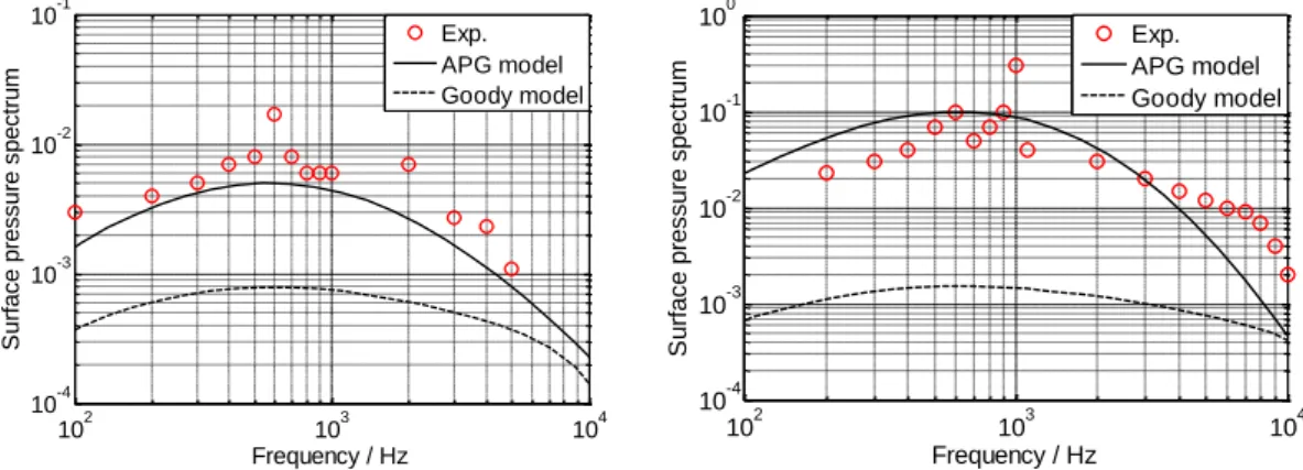
The model is validated in the original paper of Rozenberg et al (2012) against 5 different experimental results. In this paper, it is further validated against the data from DTU report (Bertagnolio, 2012). The experiments are launched in a wind tunnel with a symmetric airfoil NACA0015. Test velocities are 30m/s, 40m/s, 50m/s, and the angle of attack is 0, 4, 8, and 12 degree. The chord length c is 0.9 m, and the microphone at which wall pressure is recorded is located at x/c = 0.894. Since no detailed boundary layer parameters are provided from the experiment, XFOIL is used to calculate the necessary input parameters for the APG model. For comparison, the test velocity of 30 m/s and 50m/s at zero angle of attack case are considered. The comparison result is shown in Figure 2.
Fig. 2 Wall pressure spectrum measured by Bertagnolio (2012) (circles), and modeled by the APG model(solid line) and Goody's model(dashed line) respectively. Left, U = 30m/s; right, U = 50m/s.
4. Model validations against fixed airfoil measurements
4.1 Turbulent inflow noise validation
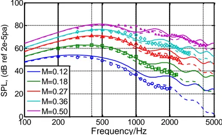
The model is compared to the experimental data from Paterson and Amiet (1976). Experiments are conducted in a wind tunnel using NACA0012 airfoil. The airfoil dimension is 0.23 m chord and 0.53 m span. The angle of attack is set to zero. The test velocities are 40, 60, 90, 120 and 165 m/s respectively, which corresponds to a free stream Mach number of approximately 0.12, 0.18, 0.27, 0.36, 0.5. The turbulence is generated by a bi-planar grid with a mesh size of 13.3 cm, the resulting turbulence intensity is of the order 4% ~5%, and the span-wise correlation length scale is around 3 cm. The noise is measured at 2.25 m radius from the
102 103 104 10-4 10-3 10-2 10-1 Frequency / Hz S u rf a ce p re ssu re sp e ct ru m Exp. APG model Goody model 102 103 104 10-4 10-3 10-2 10-1 100 Frequency / Hz S u rf a ce p re ssu re sp e ct ru m Exp. APG model Goody model
5
leading edge in the mid-span. Here the data from the microphone located directly above the leading edge are used.
The calculation results for various test velocities using large aspect ratio formulation are shown in Figure 3, with and without the leading edge thickness correction. The correction is most necessary for low Mach number at higher frequency range.
Fig. 3 SPL of turbulent inflow noise. Symbols: measurement from Paterson and Amiet (1976); solid line: without thickness correction; dashed line: with thickness correction.
4.2 Trailing edge noise validation
For the validation of trailing edge noise, the experimental data from Brooks and Hodgson (1981) are considered. The test airfoil is again NACA 0012, with a chord of 0.61 m and a span of 0.46 m. The test velocity chosen for the current validation is 69.5 m/s, and the angle of attack is zero. The reference location is 1.8 cm upstream of the trailing edge and the receiver is located 1.22 m away directly above the trailing edge in the mid-span. The span-wise correlation length that is needed for Equation (6) and (7) is determined by Corcos's model (Moreau and Roger, 2005):
with being an experimental constant, and being the convective velocity. The results for wall pressure spectrum and far field SPL are shown in Figure 4. The results from Goody's wall pressure spectrum model is also plotted for comparison with the APG model. Again we can see that the adverse pressure gradient tends to increase the far field SPL, and that the APG model provides better results than Goody's model.
Fig. 4 Comparison between APG model and Goody's model against experiment. Left: wall pressure spectrum comparison; right, far field SPL comparison.
1000 200 500 1000 2000 5000 20 40 60 80 100 Frequency/Hz SPL , (d B re f 2 e -5 p a ) M=0.12 M=0.18 M=0.27 M=0.36 M=0.50 103 104 70 75 80 85 90 95 100 Frequency / Hz pp (f )/ d B ( re f: 2 e -5 p a ) Exp. APG model goody model 103 104 10 20 30 40 50 Frequency/Hz S P L / d B ( re f: 2 e -5 p a ) Exp. APG model goody model
6
5. Results and comparison against full size wind turbine measurements
5.1 Exact formulation and sub-critical gust effect
In section 2.1, the power spectral density is simplified under the assumption of large aspect ratio. For the calculation of a wind turbine, since each blade is cut in segments on which the noise models are applied individually, it is not guaranteed that this assumption is valid for all the segments. Thus it is necessary to examine the validity of the large aspect ratio approximation for a wind turbine.
A first test on "segment aspect ratio" is carried out with a fixed NACA0012 airfoil. The chord is set to 0.5 m, and the span is set to 0.25 m, 0.5 m, 1.5 m and 2.5 m respectively, Mach number is 0.2. The observer is located in the mid-span plane 2 m above the airfoil. The results for trailing edge noise are shown in Figure 5, from which we can see that when the aspect ratio is more than 3, the simplified formula provides really close results compared to those from the exact formula. When the aspect ratio is less than 3, the main discrepancy between the two appears for frequency less than 600Hz.
(a) (b)
(c) (d)
Fig.5 Trailing edge SPL calculated by the exact and simplified formula for difference aspect ratio respectively.
The integration over ̅ in Equation (6) involves dealing with sub-critical gusts, that exists when ̅ ̅ ̅ . A set of plots of with respect to airfoil response function with respect to ̅ are shown in Figure 6. The parameters are: chord = 0.13 m, span = 0.13 m, Mach number = 0.05 and 0.3 respectively, the test frequency is 1000 Hz. The angles indicated in the figures are the observer angles in the mid-span plane, where 0omeans downstream in the airfoil plane and 90o means in direction normal to the airfoil. We observe that the airfoil response function decreases rapidly for subcritical cases when the normalized span-wise wave number increased. However, gusts with ̅ close to unity can have a significant effect on the final results. 102 103 104 5 10 15 20 25 30 35 40 Frequency/Hz S P L /d B ( re f: 2 e -5 p a ) Exact formular
Large Aspect Ratio simplification
102 103 104 10 15 20 25 30 35 40 45 Frequency/Hz S P L /d B ( re f: 2 e -5 p a ) Exact formular
Large Aspect Ratio simplification
102 103 104 15 20 25 30 35 40 45 50 Frequency/Hz S P L /d B ( re f: 2 e -5 p a ) Exact formular
Large Aspect Ratio simplification
102 103 104 15 20 25 30 35 40 45 50 Frequency/Hz S P L /d B ( re f: 2 e -5 p a ) Exact formular
7
To understand the importance of the subcritical gusts for different frequencies, the due to all the super-critical gusts and all the sub-critical gusts respectively, as well as the sum of the two are plotted in Figure 7. We can see that the sub-critical gusts are dominant at low frequency (up to 100Hz), and decrease very fast at higher frequency range. Since for the aspect ratio of 1, the simplified formula could provide satisfying results for most of audible frequency range (200Hz and above), it will be used to calculate wind turbine noise in the next section, even thought the sub-critical gusts are neglected consequently.
(a) vs ̅ , M = 0.05 (b) vs ̅ , M = 0.3
Figu.6 Airfoil response function as a function of ̅ and far field trailing edge noise. Blue line: super-critical gust,
red line: sub-critical gust.
Fig.7 SPL of trailing edge noise due to super and sub-critical gusts, M = 0.3, chord c = 0.13m, span L = 0.13. Observer in the mid-span 2m above the airfoil.
Doppler effect due to blade rotation is taken into account by relating the PSD of a moving source to a fixed source at the same instant location (Schlinker et al, 1981):
where is the Doppler factor defined by , is the source frequency and is the observer measured frequency.
5.2 Application on a wind turbine and validation against measurements
The comparison is made for a Bonus 300kW wind turbine using data from Zhu et al (2005). The main parameters for this type of wind turbine and meteorology conditions are given in Table 1. 10-2 100 -13 -12 -11 -10 -9 -8 -7 -6 -5 bK y R e la tive d B o f a ir fo il re sp o n se f u n ct io n 0o 30o 60o 90o 10-2 10-1 100 101 -7 -6 -5 -4 -3 -2 -1 bKy R e la ti ve d B o f a ir fo il re sp o n se f u n ct io n 0o 30o 60o 90o 101 102 103 104 -30 -20 -10 0 10 20 Frequency / Hz SPL / d B (re f: 2 e -5 p a ) Total SPL
SPL due to super-critical gusts SPL due to sub-critical gusts
8
Table 1 Bonus 300kW wind turbine main parameters
Rotor radius Tower Height Rotor angular speed Airfoil profile Chord length Wind speed (10m height) Observer location Ground roughness 15.5 m 31m 3.7 rad/s NACA 632xx 0.5m-1.5m 8 m/s 40m down wind 30mm
Wind shear effect is considered in the calculation by taking an experimental log law relation: (
)
where is the velocity at height , is the reference velocity at reference height , taken as the hub height here, and (Zhu et al. 2005)
(10)
is the ground roughness. The turbulence intensity
and turbulence integral length scale are calculated by the relations given in Zhu (2005), as:
and
where is the same as defined in Equation 10. The turbulence energy spectrum is calculated using the isotropic Von Kármán spectrum. Plot of the energy spectrum for integral length scale = 100 m with various turbulence intensities and a turbulence intensity = 0.1 with various integral length scales are shown in Figure 8.
(a) = 100 m (b) = 0.1
Fig. 8 Von Kármán turbulence energy spectra for different integral length scales and turbulence intensities.
The calculation procedures are the following: first, each wind turbine blade are artificially cut in several segments, here, 10 segments of 1.5m length for each blade, so that the maximum aspect ratio remains no larger than 1. According to the flow conditions at each segment, the boundary layer parameters required by the APG wall pressure model are calculated by XFOIL (version 6.96) and stored in advance. The noise models for turbulent inflow noise and trailing edge noise are then applied for each segment, with thickness correction and Doppler effect considered. The final total noise perceived by the observer is obtained by logarithm summation over all the segments.
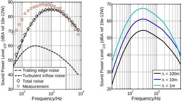
Figure 9 shows the sound power level from the calculation compared to the measurement. The results are shown in 1/3-octave bands, A-weighted and averaged over one rotating period. It is needed to say that the measured data includes all the noise mechanisms (stall noise, trailing edge bluntness noise, etc) which are not considered by the models. According to our model, trailing edge noise is dominant over turbulent inflow noise for this type of wind turbine under these meteorological conditions. The agreement between the calculation and the measurement
10-2 100 102 -60 -40 -20 0 20 Wave number K E (k) / d B I = 0.05 I = 0.1 I = 0.15 10-2 100 102 -60 -40 -20 0 20 Wave number K E (k) / d B = 50m = 100m = 150m
9
is acceptable in the frequency range of 600 Hz to 8000 Hz, but at lower frequency range, the results shows up to 20 dB differences. Turbulent inflow noise level is rather low, which might be due to the large turbulent integral length scale, that ranges between 120 m to 180 m. On the right figure, it is shown that a decrease of turbulent integral length scale will increase the noise level for a fixed turbulence intensity.
Fig. 9 Left: Comparison of turbulent inflow noise and trailing edge noise models against measurement. Right: influence of turbulent integral length scale on the turbulent inflow noise.
The comparison for trailing edge noise using APG wall pressure model and Goody's wall pressure model is shown in Figure 10. The results are shown in 1/3-octave bands. It is clear that an adverse pressure flow condition greatly increases the trailing edge noise. By using APG model, the results are much closer to the measurements. Figure 11 shows the thickness
correction for turbulent inflow noise. Under this atmospheric turbulence condition, more
precisely, when the turbulent integral length scale is much larger than the size of blade chord, this correction is not significant.
Fig.10 Comparison between APG model and Goody model for trailing edge noise.
Fig.11 Turbulent inflow noise with/without leading edge thickness correction.
102 103 104 30 40 50 60 70 80 90 Frequency/Hz So u n d Po w e r L e ve l 1/3 , (d BA re f 1 0 e -1 2 W )
Trailing edge noise Turbulent inflow noise Total noise Measurement 102 103 20 30 40 50 60 70 Frequency/Hz So u n d Po w e r L e ve l1/3 (d BA re f 1 0 e -1 2 W ) = 100m = 10m = 1m 102 103 104 20 30 40 50 60 70 80 90 Frequency/Hz S o u n d P o w e r L e ve l 1/3 / d B A ( re f: 1 0 -1 2 W ) APG model Goody model 101 102 103 104 20 25 30 35 40 45 50 55 60 Frequency/Hz So u n d Po w e r L e ve l 1/3 , (d BA re f 1 0 e -1 2 W )
Without thickness correction With thickness correction
10
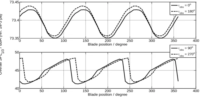
Fig.12 Total SPL variation during one period perceived at difference observer location. corresponds to the observer at
downwind direction, and corresponds to the observer at rotor plane on the left side when facing downwind direction.
Figure 12 shows the total SPL variation during one rotating period, the observer is at a 40 m distance from the wind turbine. From the result we can see that when the observer is upwind or downwind direction (corresponds to and ), the perceived SPL is almost constant; but for an observer located in the rotor plane direction (corresponds to and ), even thought the overall SPL is much less, but the variation during one period reaches up to 6 dB. These trends agree with the results from Lee et al(2013).
The directional feature of overall SPL averaged over one rotating period is shown in Figure 13. The wind is coming from the left to the right. The pattern shows a dipole shape, as was shown in many previous work (Zhu 2005, Lee et al, 2013), with a bit lower level in the rotor plane direction, and a higher level in the wind direction.
Figure 13 Directivity of overall SPL in dB(A).
6. Conclusions
Amiet's analytical model for turbulent inflow noise and trailing edge noise are extended by considering an APG wall pressure model and a leading edge thickness correction respectively. The extended models are first validated against fixed airfoil measurements, then applied to a full size wind turbine. APG wall pressure model greatly improved the accuracy for trailing edge
Ov era ll SPL 1 /3 / dBA (ref : 2e-5 pa) 0 50 100 150 200 250 300 350 400 40 45 50
Blade position / degree
0 50 100 150 200 250 300 350 400
73.35 73.4 73.45
Blade position / degree
obs = 0 o obs = 180 o obs = 90 o obs = 270 o 20 40 60 80 30 210 60 240 90 270 120 300 150 330 180 0
wind
11
noise prediction, while for the turbulent inflow noise, the thickness correction does not seem significant when the atmospheric turbulent length scale is very large. The results of total SPL as a function of blade position are expected to give an explanation for the 'swish' effect. When the observer is located at rotor plane direction, the amplitude modulation causes a strong 'swish'; while if the observer is located at upwind or downwind direction, the effect is hardly noticeable. In the future, the model will need to be compared to a more detailed wind turbine experimental campaign, since the comparison with data from the literature is not completely satisfying. Also, the model will be coupled to a propagation model and a more realistic model of the atmospheric boundary layer will be considered. Finally, other noise mechanisms that can give rise to rapid time fluctuations such as stall noise will be investigated.
Acknowledgements
The authors would like to thank Michel Roger and Yannick Rozenberg from the Laboratoire de Mécanique des Fluides et d'Acoustique (LMFA) of the Ecole Centrale de Lyon for useful discussions regarding Amiet's theory.
References
Amiet R.K (1975) Acoustic radiation from an airfoil in a turbulent stream, Journal of Sound and vibration 41(4), 407-420
Amiet R.K (1976) Noise due to turbulent flow past a trailing edge, Journal of Sound and Vibration 47(3), 387-393
Bertagnolio (2012) Low noise airfoil-Final report , EUDP project
Brooks T.F and Hodgson T.H (1981) Trailing edge noise prediction from measured surface
pressures, Journal of Sound and Vibration 78(1), 69-117
Brooks T.F, Pope D.S and Marcolini M.A (1989) Airfoil self-noise and prediction, NASA reference publication 1218
Goody M (2004) Empirical spectral model of surface pressure fluctuations, AIAA Journal 42(9) 1788-1794
Howe M.S(1978) A review of the theory of trailing edge noise, NASA Contractor report 3021 Lee S, Lee S and Lee S (2013) Numerical modelling of wind turbune aerodynamic noise in the
time domain, Journal of Acoustical Society of America, 133(2)
Moreau S and Roger M (2005) Effect of airfoil aerodynamic loading on trailing-edge noise
sources, AIAA Journal, 43(1)
Oerlemans S, Sijtsma P, Lopez B.M (2007) Location and quantification of noise sources on a
wind turbine, Journal of Sound and Vibration, 299
Paterson R.W and Amiet R.K (1976) Acoustic radiation and surface pressure characteristics of
12
Rozenberg Y (2007) Modélisation analytique du bruit aérodynamique à large bande des
machines tournantes: utilisation de calculs moyennés de mécanique des fluides. PhD thesis,
L'école centrale de Lyon.
Rozenberg Y, Robert G, Moreau S (2012) Wall-pressure spectral model including the adverse
pressure gradient effects, AIAA Journal 50(10)
Roger M and Moreau S (2005) Back-scattering correction and further extensions of Amiet's
trailing-edge noise model. Part 1: theory, Journal of Sound and Vibration, 286, 447-506
Roger M and Moreau S (2010) Extensions and limitations of analytical airfoil broadband noise
models, International Journal of Acoustics 9(3), 273-305
Schlinker R.H and Amiet R.K (1981) Helicopter Rotor Trailing Edge Noise, NASA Contractor Report 3470.
Styles P, Westwood R.F, Toon S.M, Buchingham M.P, Marmo B, Carruthers B (2011)
Monitoring and mitigation of low frequency noise from wind turbines to protect comprehensive test ban seismic monitoring stations, 4th International Meeting on Wind Turbine Noise, Rome,
Italy
Zhu W J, Heilskov N, Shen W.Z, Sorensen J.N (2005) Modelling of aerodynamically generated