Lyapunov exponents from experimental time series. Application to cymbal vibrations

HAL Id: hal-01134813

https://hal-ensta-paris.archives-ouvertes.fr//hal-01134813

Submitted on 17 Nov 2017

HAL is a multi-disciplinary open access

archive for the deposit and dissemination of

sci-entific research documents, whether they are

pub-lished or not. The documents may come from

teaching and research institutions in France or

abroad, or from public or private research centers.

L’archive ouverte pluridisciplinaire HAL, est

destinée au dépôt et à la diffusion de documents

scientifiques de niveau recherche, publiés ou non,

émanant des établissements d’enseignement et de

recherche français ou étrangers, des laboratoires

publics ou privés.

Lyapunov exponents from experimental time series.

Application to cymbal vibrations

Cyril Touzé, Antoine Chaigne

To cite this version:

Cyril Touzé, Antoine Chaigne. Lyapunov exponents from experimental time series. Application to

cymbal vibrations. Acta Acustica united with Acustica, Hirzel Verlag, 2000, 86 (3), pp.557-567.

�hal-01134813�

Lyapunov Exponents from Experimental Time Series: Application to

Cymbal Vibrations

Cyril Touze, Antoine Chaigne

Ecole Nationale Superieure des Telecommunications, Departement TSI, CNRS URA 820,46 Rue Barrault, 75634 Paris Cedex 13, France

Summary

Lyapunov exponents are among the most relevant and most informative invariants for detecting and quantifying chaos in a dynamical system. This method is applied here to the analysis of cymbal vibrations. The advantage of using a quadratic fit for determining the Jacobian of the dynamics is presented. In addition, the interest of using a time step for the evolution of the neighbourhood not equal to the timelag used for the reconstruction of the phase space is underlined. The robustness of the algorithm used yields a high degree of confidence in the characterization and in the quantification of the chaotic state.

To illustrate these features in the case of cymbal vibrations, transitions from quasiperiodicity to chaos are exhibited. The quasiperiodic state of the system is characterized together by the power spectrum of the experimental signal and by calculation of the Lyapunov spectrum.

1. Introduction

Cymbals belong to the category of non linear percussion in-struments. In their normal use, these instruments are struck by a mallet. Pairs of cymbals can also be struck against each other, especially in bands or in orchestral use. Due to the rather heavy strokes, the vibrations of cymbals generally exhibit large amplitude, compared to their thickness, which leads to nonlinear effects. As a consequence, the pitch of such instruments is not clearly defined. Only at the end of the de-cay, as the magnitude of the motion becomes sufficiently small, one can clearly hear the most salient eigenfrequencies of the normal modes predicted by the linear theory. Previ-ous investigations on cymbals are mostly concerned with the linear regime [ 1], and only a few references address the ques-tion of nonlinearity which is of prime importance for these instruments [2, 3]. In order to tackle this problem, one strat-egy consists in investigating the underlying physics of the vibrating structure. This method has been applied to gongs in the past [4, 5]. One complementary approach is to inves-tigate the dynamical behaviour of these instruments with the help of nonlinear signal processing tools. This is the purpose of the present paper.

The main difficulty for the analysis of struck cymbals fol-lows from the broadband excitation of the initial pulse. This pulse excites simultaneously a very large number of frequen-cies, in a very short amount of time, which makes it almost impossible to analyse the successive bifurcation mechanisms and the routes to chaos. In addition, the magnitude and loca-tion of the pulse is generally hard to reproduce. Therefore, it seems more appealing to drive the cymbal with slowly and continuously increasing magnitude, so that transitions from the linear to the chaotic state can be observed, and to limit the spectrum of the excitation. In practice, the cymbal is driven here sinusoidally at frequencies close to the most

salient linear eigenfrequencies of the instrument, or inten-tionally apart from these eigenfrequencies [6]. The velocity of one selected point of the instrument is recorded during about three minutes (see Figure 5). At large amplitude, it is interesting to notice that the sound obtained by driving the cymbal with a sinusoid instead of a pulse is clearly com-parable to characteristic cymbal sounds, although the tone quality may be somewhat poorer. This is a strong argument in favor of considering the typical sounds of the instrument in ordinary performances as a combination of the nonlinear effects due to a limited number of active modes.

In this paper, particular attention is paid to the calculation of the Lyapunov exponents from experimental time series. The method used here for computing the Lyapunov spec-trum relies on an idea conjointly developped by Eckmann and Ruelle [7, 8] and Sano and Sawada [9]. This method consists of approximating the matrix of the linearized flow in the reconstructed tangent space. One major advantage of this method is that, in theory, the complete spectrum of the exponents can be obtained. Other methods, in which the di-vergence of nearby trajectories is used, are also possible can-didates, but their principal.limitation follows from the fact that, in practice, only the maximal exponent can be obtained [ 10, 11]. Other methods, based on a global reconstruction of the vector field and especially designed for short or noisy data sets, are also available [12, 13]. These methods will not be considered here.

The main features of the algorithm presented in this paper are the following: first, the local Jacobian of the evolution function in the reconstructed tangent space is approximated by a higher-order local polynomial [14, 15, 16]. As a conse-quence, it is expected that the accuracy in the determination of the negative exponents will be improved, and that the presence of spurious exponents, multiples of the true expo-nents, will be avoided. One example of the existence of such spurious exponents was first noted in [8]. More recently, an analytic proof has been given by Sauer et al. [ 17]. Second, a time step for the evolution of the neighbourhood is selected,

which is different from the timelag used for the reconstruction of the attractor. This improves significantly the detennina-tion of the exponents. These properties of the algorithm will be illustrated numerically on standard computer-generated time series originated from chaotic discrete and continuous dynamical systems.

Interpretation of the Lyapunov exponents related to real world data is a rather difficult task which should be done with great care. However, a number of successful applications can be mentioned, which cover various fields of physical systems: hydrodynamics [8], chemistry [10], fundamental physics [ 18, 19] and acoustics [20, 21]. including musical acoustics [22, 23], and speech [24]. In section 3 of the pa-per, the computation of the Lyapunov exponents is appbed t.o experimental time series obtained from measurements per-formed on a thin crash cymbal, which is driven sinusoidally at its center by means of

a

shaker. Similar experiments were conducted in the past by Fletcher. Rossing et al. [3, 5, 2]. By increasing slowly the amplitude of the shaker motion, transi-tions from linear to chaotic motion are observed. A complete description of the experimental setup can be found in [6}, together with the results of the algorithms used for estimat-ing the dimensions of the system (correlation dimension, and false nearest neighbours). The calculation of the Lyapunov exponents makes it possible to detect the presence of chaos,

and to quantify the "degree of disorder" in the chaotic regime. In addition. this analysis gives us a better understanding on the route to chaos observed in the system, through testing of the quasi periodicity of the measured signal. This point will be developed in section 4.

2. Calculation of the Lyapunov spectrum 2.1. Algorithm

The methods of current use in nonlinear signal processing are based on the Takens reconstruction theorem [25]. Recent surveys present both the theoretical background and appli-cations of these techniques for chaotic signals [18, 19, 26]. Therefore, the fundations of this theory will not be developed further in this paper.

In order to compute the Lyapunov spectrum of a given time series, it is necessary to obtain the local Jacobian of the underlying now from the trajectory in the reconstructed phase space. The principle is the following: Given a time series {s(n)}n=l. .. N. a multivariate trajectory is formed with a timelag T and a so-called embedding dimension d5. The value of the timelag is usually taken as the first minimum of the Average Mutual Information function [27]. A lower bound for the embedding dimension can be given by using the test of the false nearest neighbours [28]. This yields the vector:

y(k) = [s(k), s(k

+

T), ... , s (k +(dE-

l)

T)]

.

Denoting F the evolution function which maps the vector y(k) onto the vector y(k

+

Tp), one can write:

y(k

+

TF) = F(y(k)), {1)

where TF is the time step for this local neighbourhood-to-neighbourhood mapping. The main task of the algorithm is to compute the local Jacobian matrix DF(k) in the tangent space, since the Lyapunov exponents are computed from the eigenvalues of the Jacobian.

Defining further:

• {y{k;)} i=I. .. Nv: the Nv nearest neighbours ofy(k),

• TJ(k, i) = y(k;) - y(k), i ;:; 1 ... Nu: the small dis-placements in the neighbourhood ofy(k),

• TJ(k+Tp,i) = y(k; +Te) - y(k+Tp),i = 1 ... N11 : the small displacements in the evolved neighbourhood, after T F time steps,

the local Jacobian is then calculated via a Taylor expansion in equation (1). The standard method consists in Iinearizing F, but it has been found that higher-order Taylor expansion give better results [16].

A second-order expansion, for example, with i = 1 ... N11 , yields:

TJ(k

+

Tp, i) =

(2)

DF(k)ry(k, i)

+

~ry

(

k,

i)t

H

(k)

ry

(k,

i) where

(8

F

·

)

DF(k);,; =

B

y;

(y(k))

is the Jacobian of the evolution function F, and

( 82F; )

H(k);,;,t = fJyjl)y, (y(k))

is the Hessian of

F

.

Equation (2) is then projected onto a subspace of dimen-sion dL

5:

de. de- is the local dimension corresponding to the dimension of the manifold on which the dynamics takes place, which should not be mistaken for the embedding di-mension dE. The dimension dE should be large enough so as to avoid the presence of false neighbours [ 18, 19]. All sub-sequent calculations are made in a dL-dimension subspace, which provides us with d1, Lyapunov exponents.

The next step of the algorithm consists in calculating DF and H through matrix inversion corresponding to equa-tion (2) (the Hessian part can be written in a matrix form. See, for example. [ 16) for more details). The coefficients of H are useful only for assessing the trajectory, since the Lya-punov spectrum is computed from the eigenvalues of DF. Thus, only the Jacobian part is finally retained.

The last step of the algorithm is the classical QR decom-position of the Jacobian, which is evaluated along the phase space trajectory, in order to calculate the dL Lyapunov ex-ponents [7]. With K the number of points on the attractor for which the Jacobian has been estimated, R(k) the R matrix from the QR decomposition at y(k ), and T the sampling time step, the itlt Lyapunov exponent is given" by:

This summary of the main steps of the algorithm shows that many parameters are involved: T and dE for the reconstr uc-tion, Tp, dr" K and Nv for the fit. For most of them, simple rules are clearly established to avoid pitfalls. A large number of references exist in the literature devoted to non linear signal processing where the rules for selecting appropriately these parameters are specified (see, for example, [18, 19, 29]).

2.2. Higher-order Taylor expansion

Most of the algorithms used for estimating the local J aco-bian matrix restrict the Taylor expansion of equation (l) to the first-order (linear) term. In the present study, the use of higher-order expansions has been investigated. The major expected improvement is to increase significanrly the accu-racy of the result~, especially for the negative exponents for which the linear algorithms present a number of difficulties [15, 16]. Two simultaneous burdens result from a linear fit on the Jacobian since, first, the trajectory must be approximated and, second, the Lyapunov exponents must be given. Using a higher-order expansion implies that all terms in the matrices of equation (2) are involved in the approximation of the local neighbourhood-to-neighbourhood mapping.

The accuracy of the results does not increase monotoni-cally with the degree dp of the expansion. This feature can be explained as follows: with increasing dp. it is necessary to take a larger number of neighbours into account in or -der to perform the matrix inversion in good conditions. As a consequence, the assumption of small neighbourhood for the Taylor expansion is not verified any more. In other words, the number of selected neighbours Nv for computing the ma-trix must be large enough to overcome numerical instability, but, at the same time, this number is limited in order to keep the neighbourhood as small as possible. A good compromise consists in selecting Nv is given by [16]:

Observations made by computing a third-order expansion of equation (1) show that the accuracy of the results is not significantly improved, compared to the second-order one. Therefore, it has been decided to select a second-order

ex-pansion.

Another important fact that justifies the use of a second-order expansion is linked to the problem of spurious e xpo-nents. One major problem, when dealing with experimental time series, is that the local dimension of the attractor, and thus the number of Lyapunov exponents, is not known. As a consequence, if the dimension is too large, then the algorithm presented in section 2.1 generates spurious exponents. With a first-order expansion, for a noise-free case, it is found that some of the spurious exponents arc integer multiples of the true ones, as noted in [8] and demonstrated in [17).

With a second-order expansion, still for a noise-free case, the presence of tJ1ose spurious exponents which are multi

-ples of the true ones, is avoided. With a linear fit, a spurious exponent equal to twice the positive one appears as the local

Table I. Calculated Lyapunov exponents for the Henon map, with linear and quadratic fits. The length of the sequence is equal to

40000 points, with T

=

TFTT

=

1 for a discrete map, dE

=

8

and K=l200. The apparition of a spurious exponent at twice the true positive one

>.

1

= 0.418, with the linear fit, is clear. The second theoretical exponent is

>.2

=

- 1.621. With the quadratic fit, the spurious exponents are all negatives.

dL Lyapunov exponents, linear fit

2 0.41468 -1.62298

3 0.41585 -0.59021 -1.63580

4 0.74228 0.40747 -1.58824 -1.86754

5 082522 0.41393 -0.87694 -1.57883 -1.97449

dL Lyapunov exponents, quadratic fit

2 0.41951 -1.62404

3 0.42024 -0.87376 -1.62046

4 0.41806 -0.48700 -0.87292 -1.62386

5 0.41866 -0.31485 -0.44684 -0.86411 -1.61900

dimension dL increases. This phenomenon may lead to the incorrect conclusion that two positive exponents exist in the system. By using a quadratic fit, those false multiple posi-tive exponents are avoided. Despite our efforts, no analytical proof of this property could be given. Indeed, the mathe-matical derivations leading to the analytic result of [17], when extended to the quadratic case, give a system which bears an implicit solution [30). However, a number of nu

-merical calculations performed on different systems (Henon map, logistic map, Lorenz system) show that the quadratic fit eliminates the multiple spurious exponents. This feature is illustrated for the Henon map in Table I.

2.3. Selection of the evolution time Tp

Selecting an appropriate value for Tp is a particularly hard task in the case of continuous-time dynamical systems. Previ-ous algorithms use Tp = T as a general feature (8], because it substantially simplifies the implementation. However, there are no other justifications for this choice, and thus it is not recommended to select Tp = T, since there are no relations between these two quantities, as mcntionned in [16]. The choice of Tp is directly connected to the choice of the dis-crete map which best fits the continuous How, and no general rules are available for this problem.

However, for too small evolution time Tp, the local con-traction or expansion properties of the How arc not well taken into account, thus leading to a bad estimate of the whole spectrum. On the contrary, when Tp approaches T, there is some probability for the trajectory to be too smoothed, hence leading to underestimate the negative exponents.

By studying the effect of Tp on a number of continuous maps, it has been observed that using a too small Tp leads to poor results, and that the precision of the estimated Lyapunov spectrum becomes acceptable as TF

2:

T /2. This feature is illustrated on a time series generated from the forced Duffing

0.2r--~-~-~-~~-~-~-~-~--., (I.[ ~ () c ·- -0 I ~-~ -0.2 ° c 8..-tl.3 :5 > -0.4 0 § -0.5 c.. ~-0.6 ...:l -0.7 ... 0. .... 0 2 4 5 6 7 lO Evolution time Tp

Figure 1. Lyapunov equation for the Duffing equation, as a function of the evolution time TF. The parameters are K = 2000, T = 10,

dE= 6, and dL = 3. 40000 points have been used for the calculation, with a quadratic fit. It can be seen that the acceptable values for the evolution time are obtained for TF :::: T

/2.

The true exponent are marked by dotted lines.

equation:

x

+

8x

+

x

+

x3

=

a cos(wt)

with 8

=

0.2, a

=

40, w

=

1. For this choice of parameters, the Lyapunov exponents are .A1

=

0.11, .A2

=

0, A3

=

-0.31 (in s-1) [31]. The time series was calculated with initial conditions: x = 1 and ;i; = 0.7. The length of the series is equal to 40000 samples. The first 5000 samples were cut in order to avoid the influence of transients. A fourth-order Runge-Kutta method is applied to the system, with a sampling time step of 0.04 s. For this value, the first minimum of the Average Mutual Information function is obtained for

T = 10 samples. In this example, Figure I shows that the best spectra are obtained for Tp

2:

T /2. It has been found that this empirical rule remains valid for higher embedding dimensions.

In a second set of experiments, a time series obtained from the first coordinate of the Lorenz system, sampled by a fourth-order Runge-Kutta scheme, has been used. The sam-pling time step is equal to T = 0.01 s. In this case, the first minimum of the Averaged Mutual Information function is equal to 0.1 s, which corresponds to T = 10 samples. Fig-ure 2 shows that in this case, the best spectrum is obtained

forTp = T/2.

In conclusion, it turns out that even if no general rule can be asserted, all particular cases investigated show that selecting Tp :::; T /2 leads to bad results.

2.4. Results on computer-generated time series

In order to check its validity and limits, the algorithm has been tested on computer-generated time series derived from well-known dynamical systems (logistic, Henon and Ikeda maps, Lorenz and Rossler systems, Duffing equation, super-position oftwo incommensurate sinusoids). In each situation,

0 -~: :::::::::~: :::::::::~: :::::::::~:.::·::::::~: :.::.::·:~: ::::::·::~: :::::::::~: :::::::::~: :::::::::~· -5 in .S-10 i@-15

"'

c g_-20 K ~-25 0 §-30 ~ .s-35 -40 + ~-~2--~3~~4--~5--~6--~7--~8--~9--~1~0 Evolution time Tp

Figure 2. Lyapunov exponents for the Lorenz system, as a function of the evolution time TF. The optimal value for TF is T

/2.

The calculation has been made with 40000 points from the first coordinate of the Lorenz system, with K = 1500, dE = 4, dL = 3, and T

=10. The true exponents are marked by dotted lines. A quadratic

fit has been used. The influence of TF is particularly visible on the negative exponent (marked by a(+)), whereas the positive one and the vanishing one((*) and (o)) do not vary significantly with TF.

0 -1 "' .5 ri -2 c

"'

c 0 c.. :5 > 0 c

=

~

.s

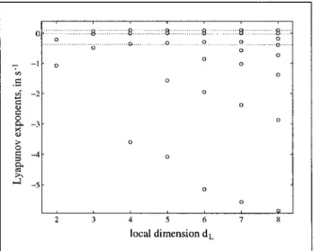
-3 -4 -5 ·::::::::s:. :::::·:·:::::2 ... :::::8: ·::::::::::::8 ... :::·:·:8 ... :::::8:'" 0 ... g.,, 0 ... Q. .... 0 0 0 0 0 0 0 0 0 0 4 5 6 local dimension dL

Figure 3. Lyapunov exponents for the Duffing equation as a function of the local dimension dL, with K = 1400, T =10, TF =6, dE =8.

The true exponents are marked with dotted lines.

a quadratic fit has been used. It is found that the true Lya-punov exponents are estimated within I%. Only the two last examples (Duffing equations and incommensurate sinusoids) will be presented below. The first example is aimed at illus-trating the performance of the method on a chaotic system, and the second example shows that the method used also yields excellent results with a non-chaotic signal.

Figure 3 shows the computed Lyapunov exponents for increasing values of dL, with the time series used in the pre-vious section. The evolution time is here Tp= 6 samples. The convergence ofthe true exponents (marked by dotted lines on Figure 3) with increasing dL is clear, whereas the spurious ones vary with d£. This can help in identifying the

spuri-ous exponents. This figure shows that the absolute value of the false exponents is systematically larger than the absolute value of the largest true one. However, this property cannot be generalized. Tests performed on the Lorenz system, for example, show that the spurious exponents obtained in this case are also all negatives, but that they are located between the vanishing exponent and the most negative one. These results are in accordance with those previously obtained by other authors [8, 16, 20, 32]. From these observations, one is led to conclude that it is not possible to exhibit a general rule for the location of the spurious numerical exponents in the Lyapunov spectrum.

A signal composed of two incommensurate audible fre-quencies has been also tested. The results show that the algorithm is robust for finding the two-torus on which the trajectory takes place, by exhibiting two clearly vanishing exponents whatever the local dimension d£. The signal is made of the following frequencies:

fi

=

440Hz and

h

=

2v'2JI

=

1244.5 Hz, with equal amplitudes. A trajectory of 40000 points has been used, with a sampling frequency Fe

= 48000 Hz, a standard value for audio signals. The delay T for the reconstruction is equal to 16 samples. Figure 4 shows the convergence of the exponents, for a local dimension dL equal to 3. The signature of a two-torus is assessed by the presence of two zero exponents, while the remaining ones are all negatives.

A commonly accepted method to discriminate the spurious exponents consists in computing the Lyapunov spectrum for a given time series, read first forward and then backward in time [31]. The expected behaviour is that the signs of the true exponents change with time reversal, whereas the spurious ones do not. This method has been found to give excellent results with time series issued from discrete maps (Henon, logistic and Ikeda map has been tested in this manner), thus leading to an undoubted identification of the spurious ex-ponents. Unfortunately, in the case of continuous flows, the expected behaviour is not so clearly visible, and the iden-tification of true and spurious exponents becomes slightly impossible. Thus, this method was not used in the present study.

3. Application to the cymbal

3.1. Experimental set-up

The previously described method for determining Lyapunov exponents has been applied to experimental time series on a Zildjian thin crash cymbal (diameter: 41 cm), in order to as-sess and quantify the chaotic regime. In this experiment, the cymbal is clamped at its center to an impedance head (B&K 8001) mounted on a LDS vibration exciter. The amplitude of the driving force is slowly and linearly increased by modu-lating the sinusoidal driving signal by a triangle waveform of very low frequency. The magnitude of the driving force lies within the range 1 to 20 N, depending on the driving frequency. The magnitude of the displacement at the edge is generally between 0.1 and 1 mm. However, this magnitude

0.02,---~---~---,

·=

"' ;:

_g

-0.(14 0 0.. ><

"'

;> 0 c:

!~"

r

-0.120 51Kl HKKl 151Kl Number K of iterations

Figure 4. Convergence of the Lyapunov exponents with the num-ber K of iterations for a signal composed by two incommensurate frequencies. The two first exponents are equal to zero, the third one (spurious) is negative, which is consistent with the theoretical results. The fixed parameters are: dE= 6, dL = 3, T = 16, TF = 10.

\) 2 3 _{t in minutes}

Figure 5. Global temporal shape of the signal recorded at the edge of the cymbal, with driving frequency Fexc

=

412Hz. The amplitude of the excitation is slowly and linearly increased until 2 min 40 s, time at which the driving force is suddenly removed.

may become very large for some values of the excitation frequency. In ce1tain cases, edge displacements up to 1 cm have been observed. The analyzed signal is delivered by an accelerometer (B&K 4393) glued either at the edge or at a distance of r /2 from the center, where r is the radius of the cymbal, and recorded on a DAT-tape with sampling fre-quency Fe

=

48000 Hz. The duration of the recordings lies between 2 and 5 minutes. One example of recorded signal is shown in Figure 5. Sharp transitions can be seen on this figure, as well as the relaxation effect after suppression of the excitation, around t

=

2 min 40 s. In order to observe various types of transitions, the forcing frequency is either close to one linear eigenfrequency of the cymbal, or signif-icantly apart from eigenfrequencies and from low-order lin-ear combinations of these frequencies. In a previous work, calculations of the correlation dimension and of the embed-ding dimension, by means of the false nearest neighbours method, have been performed on these signals. The results show, among other things, that the dimension of the under-lying dynamics is less than or equal to 7 [6].

As it is generally the case for experimental signals, when

compared to computer-generated series, for example, the present signals exhibit a finite signal-to-noise ratio (typically 50 dB). This signal-to-noise ratio is essentially due to the

ac-celerometer. Moreover, the reconstruction does not display a

clear fractal form. Since the algorithm makes extensive use

of the geometrical properties of the phase portrait (neigh

-bouring trajectories), some difficulties may be encountered

in the detennination of the exponents. To illustrate this, a

two-dimensional reconstruction is shown in Figure 6, for a

driving frequency Fexc

=

526Hz, after the onset of chaos.

3.2. Results

The results presented below were obtained in the large ampl

i-tude vibration regime, characterized by a dense and broad

-band Fourier spectrum. In fact, one primary goal of this

study was to assess that the cymbal vibration was really chaotic. Thus, the convergence of a positive Lyapunov expo

-nent was expected. Calculations of the Lyapunov exponents

were made for four different driving frequencies and for two

different locations of the accelerometer. In each situation, a

portion of 40000 points of the signal is selected (which

cor-responds to a duration of 0.83 s), once the chaotic regime is

well established. In Figure 5, for example, a portion of 0.83 s

was selected around 2mn30s. At that time, the driving force

is typically equal to 10 N.

A typical curve of convergence is shown in Figure 7. This curve has been obtained for particular values of the involved set of parameters. It has been checked that the best

conver-gence is obtained for Tp around T /2 as shown previously

on calculated time series. It is observed that the convergence

is less pronounced as Tp is equal to T. One can notice,

in particular, the convergence of the largest exponent, for in

-creasing values of dL, which clearly indicates the presence of

a positive exponent in the system. Thus, it. can be concluded

that the vibration is chaotic. One problem arising from the

blurred trajectory of the experimental signal is that spurious exponents appear at positive, though relatively small, values.

In order to validate the analysis, the results obtained are

checked against theoretical rules given by different authors:

• The Kaplan-Yorke conjecture [33] yields a dimension

dKY from the spectrum of the Lyapunov exponents

de-fined by:

d N

L:

~

1

Ai

I<Y

=

+

IAN+ll

where N is such as:

L:~

1

Ai

>

0 and

L:~t

1 Ai

<

0.

This dimension dJ<y can be used in comparison to the

correlation dimension d2 [34, 6] in order to get confidence

in the calculated exponents. This also yields a guideline

for the· selection of the local dimension dL.

• Theoretical results show that, when computing the L

ya-punov spectrum from a time series derived from a contin

-uous dynamical system, at least one vanishing exponent must be present which represents the continuity of the

trajectory. X 10 4

~0

-I -I 0 s(t)

Figure 6. Trajectory in the reconstructed phase space, with T

=

16, for nn acceleration signal of the cymbal driven at 526Hz, once the

chaotic regime is established. 0.02 ... o ... () ........ 0 ................. Q ... o ... 0 0 0 0 0 ... g _{............ ·-···o·····} ···e··· ···~ _{................ a} 0 0 ... 0 0 0 0 0 0 0 0 0 0 0 0 -o.l2 0 0 5 6 local dimens-ion<\._ 7

Figure 7. Lyapunov exponents in (sample)-1, as a function of the

local dimension dL, for the acceleration signal recorded at the edge

of the cymbal driven with Fexc = 526Hz. 30000 points are used for

the analysis. The parameters have the following values: dE = 8, K

=

2000, T

=

16, TF = 10. A clear convergence to 0.020 is observed for the largest exponent.

However, applications of theses rules show that one cannot

conclude with absolute certainty on the validity of all L ya-punov exponents. Table 11 shows the results obtained for an acceleration signal recorded at the edge of the cymbal, with

Fexc = 526 Hz. These results are also shown in Figure 7 for

dL E [3, 8). The correlation dimension for the same signal

has already been calculated, which gives d2 = 3.6 (6). Com

-paring this value with dKY calculated with the Lyapunov exponents shows that, for dL

2:.

6, dKY becomes too large

compared to d2

=

3.6. Thus, the best candidates for the

spec-trum are obtained for dL equal to 4 or 5. At this stage, it

spec-Table 11. Calculated Lyapunov exponents for three different values of the local dimension dL. for the cymbal driven at526 Hz, and with the acceleration measured at the edge. The length of the experimental sequence is equal to 40000 points. The other fixed parameters are: ds = 8.

T = 16, TF = 10, K = 2000. The exponents are given here in normalized units with respect to the sampling time, i.e. in sample-1_.

dL Lyapunov exponents (in sample -I) _dKY

4 0.01936 0.00157 -0.00130 -0.06571 3.12

5 0.01979 000349 -0.00334 -0.01989 -0.09271 4.02

6 0.02060 0.00625 -0.00088 -0.00938 -0.03393 -0.10969 4.55

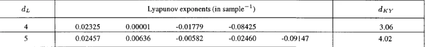
Table Ill. Calculated Lyapunov exponents in sample-1 for the cymbal driven at 412Hz, with a time series of 40000 points. The fixed parameters are: ds

=

8. T

=

I 0, TF

=

8, K

=

2000.

dL Lyapunov exponents (in sample -I) dKY

4 0.02325 0.00001 -0.01779

5 0.02457 0.00636 -0.00582

Table IV. Correlation dimension d2 , embedding dimension ds and greatest Lyapunov exponents .X. in (ms)-1, for four different driving

frequencies. Each Lyapunov exponent calculation has been made with a time series of 40000 points, using a quadratic fit.

Feo;c (Hz) Recording d2 dE .X (ms)-1 Position 412 r/2 3,4 5 1,15 ± 0.01 412 edge 2,9 5 0.82

±

0.02 440 r/2 3,8 5 I, 38 ± 0.02 526 edge 3,6 5 0, 94 ± 0.01 385 edge 4,6 7 0, 75

±

0.01 385 r/2 4,5 6 1.42 ± 0.06

tra is the most valid. A similar discussion can be made for Fexc = 412Hz. Table Ill shows the results for dL = 4 and 5, which are here also the best possible candidates. Appl

ica-tion of the rule related to the p resence or not of a vanishing exponent in the spectrum could lead to the conclusion that

the exponents obtained with dL = 4 are right. However, the correlation dimension of this signal is equal to 3.4, and thus the Lyapunov spectrum calculated with dL = 5 cannot be completely rejected.

In view of the results obtained in the two typical cases pr e-sented in Table ll and in Table Ill, one can be confident in the estimation of the largest exponent but not in the relevance of the other exponents in the spectrum. For these reasons, it has been decided to limit the present analysis to the convergence of the largest exponent.

The results obtained for four different driving frequencies are summarized in Table IV, together with the correlation dimension d2 and the minimum embedding dimension dE to use, given by the false nearest neighbours. This Table shows that a positive Lyapunov exponent has been found in each case, which is certainly the strongest indication that the sys

-tem really exhibits chaos, since the calculation of Lyapunov exponent is more reliable than the correlation dimension.

-0.08425 3.06

-0.02460 -0.09147 4.02

The precision given in this Table for the largest Lyapunov exponent is just the stan dard deviation calculated on the last I 000 iterations. The calculations are made typically with K E [1500, 2500] iterations, and the convergence is obtained in less than 1000 iterations. Figure 4 shows an example for a theoretical case (two incommensurate frequencies), where

it turns out that 1500 iterations are largely sufficient for the convergence. Finally, it can be noticed in Table IV that the exponent<: are of the same order of magnitude for all different driving frequencies.

4. Route to chaos

4.1. Ruelle-Takens theory

In this section, attention is paid to the characterization of ex -perimental transition scenarii from quasiperiodicity to chaos observed in the vibrations of the cymbal submitted to sinu -soidal driving force with increasing amplitude. Calculation of the Lyapunov spectrum during the transition, as well as power spectrum analysis, are used for identifying the route

to chaos observed. This section starts with a brief survey on

the Ruelle-Takens theory. The interested reader is referred to dedicated references for a complete description of the most classical routes to chaos and of their general properties (see, for example, [35, 36]). Specific routes to chaos (such as pe-riod doubling, quasiperiodiciry, intermittencies, crises, ... )

have been extensively studied in the past, on both theoretical and experimental viewpoints. These routes show, in parti c-ular, that the underlying mechanisms are governed by some universal laws. In this context, the Ruelle-Takens theory pos

-tulates that a limited number of Hopf bifurcations are in

-volved in the transition from a stationary state to a chaotic state, for any physical system [37, 38]. In other words, this theory establishes that, if a system exhibits three Hopf bif

ur-cations, then there is high probability for this system to be chaotic with a strange attractor.

Table V. Calculated Lyapunov exponents before the onset of chaos, for the cymbal driven at Fexc =440Hz. The acceleration is measured at

r/2. The presence of two vanishing exponents is clearly observed (the first two ones), indicating the presence of a two-torus. The motion is quasi periodic. dL Lyapunov exponents (in sample -I) 2 0.00034 -0.01823 3 0.00104 0.00006 4 0.00095 -0.00025 5 0.00063 -0.00032 6 0.00039 -0.00014 2500 i=' ₊ 0 1D 0 ~ ~-20 :::J -0.11245 -0.04235 -0.03498 -0.02134 -0.14653 -0.07654 -0.17654 -0.04657 -0.08675 -0.18659 ~ -2500

t::~~~

~~

~

~

--~

~~

~~

~

-2500 2500 500 1 000 1500 2000 2500 3000 Frequency (Hz) 4000 i=' + ~ 0 Cl) 1D 0

:s

~-20 :::J ~-40 E

.,

-3500 -4000 -2000 2000 ~o~~~~~~~~~~WL~ 500 1 000 1500 2000 2500 3000 Frequency (Hz) 5000 i=' .± 0 7i) -5000 -5000 0 S(t) 5000 500 1 000 1500 2000 2500 3000 Frequency (Hz)

Figure 8. Reconstructed trajectory and

power spectrum at three successive instants of time, showing three typical phases of the

transition to chaos. The cymbal is driven at Fexc = 440Hz and the acceleration is

recorded at r

/2

.

In physical systems, the following characteristic features

are thus expected, as the control parameter of the system in -creases (in our case, the magnitude of the driving force):

Initially, The power spectrum of the observed variable (here,

the acceleration of a given point on the cymbal) shows one

peak at a given frequency

!I

(plus, eventually, some harmon -ics). The phase portrait will be a simple closed curve, theLya

-punov spectrum will display a single zero exponent, the other

ones being negatives. Then, after a first Hopf bifurcation, the

Fourier spectrum is made of two frequencies

fi

and

fz,

and,

in addition, of all combinations

f

=

md

1

+

m2!z.

with

(m 1 , mz) E Z2. The phase space trajectory is located on a

two-torus. At this stage, one should make a clear distinction between two cases. The first case corresponds to mode lock -ing which occurs when the ratio between the two frequencies

ft

and

fz

is rational. As a consequence, the trajectory on the

torus will close itself after a finite number of cycles. In the

second situation, the ratio between these two frequencies

is irrational: the frequencies are incommensurate, and thus

the torus is densely covered by the trajectory which never

closes itself. In this case, the Lyapunov spectrum exhibits

clearly two zero exponents. When the third Hopf bifurcation

is about to appear, the phase portrait shows typical foldings, indicating that the two-torus will be destroyed, and hence that the system will gain an additional dimension [39, 40]. If

another Hopf bifurcation arises (i.e. if a third frequency

fa

is

to appear in the power spectrum), then a "broad-band noise", which is characteristic of chaos, is observed, and the torus breaks up in favor of a strange attractor. It will be shown

in the next section that the experimental signals recorded on the cymbal show, to variable extent, all the abovementioned

characteristics.

A clear survey of the transition scenarii can be found

in [35]. Details on the quasiperiodicity routes to chaos are studied in [41, 42].

4.2. Mode-locking and quasiperiodicity

Figure 8 shows the phase portrait and the power spectrum of the acceleration signal recorded on the cymbal at r /2, at three successive instants of time. The driving frequency is Fexc = 440 Hz. In the first raw of the figure, the vibratory motion of

10 0 -10 <:f + ._M

,.,

...

-~-20 Ql :3-0 ]-30 Q. ._M ,_N I + ~-

..

-e

< -40

_{_}

... N -SO

--

+ "' I -60 -70 200 400

I~

+ . _ - ...,.N 7 V) ,_t:i + ~

':f-600 Frequency (Hz) 800 1

the cymbal is weakly nonlinear. The power spectrum shows

a peak at

f

= Fexc. and some harmonics. The reconstructed

trajectory is a simple closed loop. The Lyapunov spectrum

exhibits one vanishing exponent (,\

=

0.0

±

w

-

4_{, corre}

-sponding to the continuity of the flow), the other ones being

negatives. By increasing the amplitude of the driving force,

a Hopf bifurcation occurs. Therefore, a second frequency

and combinations between Fexc and this new frequency

be-come visible. The motion is quasi periodic. The phase portrait

displays typical foldings indicating that the trajectory is l

o-cated on a two-torus which is about to be destroyed. With

increasing amplitude, a second bifurcation is observed, and

a broadband spectrum indicates the onset of chaos, as it can

be seen on the phase portrait also.

A zoom on the low-frequency part of the power spectrum

in the quasiperiodic state is shown in Figure 9. The

iden-tification of a quasiperiodic motion can be made here by

noticing that all frequency peaks, in this part of the

spec-trum, can be written as the combination

f

=

m

1

h

+

m2h,

with

h

= Fexc :::: 440 Hz, and another fixed frequency

h

::::

698 Hz. This frequency

h

corresponds here to one particular

eigenfrequency of the cymbal. This result is in accordance

with one possible interpretation of the Ruelle-Takens

sce-nario presented in [36): the Hopf bifurcation occurs when

one mode of the system is destabilized and becomes active

(ie the real part of the eigenvalue of this eigenmode

be-comes positive). The vibratory motion is then governed by

two incommensurate frequencies. Calculations of the

Lya-punov exponents were made just before the onset of chaos.

The Lyapunov spectrum clearly displays two vanishing

ex-ponents (see Table V). This indicates that the trajectory is

located on a manifold topologically equivalent to a two-torus

and confirms that the transition to chaos is obtained by the

break-up of a two-torus. If another eigenfrequency becomes

active with increasing amplitude, then the motion becomes

chaotic, as shown in the last raw of Figure 8, and as has been

1000 ._N I

...

-..,. 1200

Figure 9. Power spectrum of the previous signal be

-low 1200 Hz during the quasiperiodic state, with

Fexc =440Hz. All frequency peaks can bewrittenas

linear combination of

h

= Fe:r.c and

h

=698Hz,

where

/2

corresponds to one eigenfrequency of the

cymbal.

shown by the presence of one positive Lyapunov exponent

(see section 3).

Similar observations and calculations were made for other

driving frequencies, for which there is no evident relation

-ship with the eigenfrequencies of the cymbal (Fexc = 412,

526 and 385 Hz have been tested). Moreover, experiments

at a fixed level of excitation (which is sufficient to reach the

quasi periodic state), and with slight variations of the excita

-tion frequency, have been conducted. Hysteresis cycles were

clearly observed, with different resonance curves, depending

on Fexc is increased or decreased.

Finally, some experiments were conducted with a

driv-ing frequency equal to twice one particular eigenfrequency

of the cymbal. In this case, as expected, the following

be-haviour is observed: a mode-locking occurs between Fe:xc

and the eigenfrequency defined by fa. = Fexc/2. This result

can be seen in Figure I 0, where the driving frequency is Fe:xc

::::248Hz, and the eigenfrequency corresponding to the (4,0)

mode of the cymbal is 124Hz. An energy transfer from the

low-frequency to the high-frequency range is clearly visible

in the power spectrum shown in figure I 0. Here, the motion

is phase-locked in a ratio 2: I. As the amplitude ofthe forcing

frequency increases, the system suddenly changes to chaotic

behaviour which is characterized by a positive Lyapunov

ex-ponent, as it has been shown in Section 3 (,\ = 0.3

±

0.1

(ms)-1_{. This value was not reported in table IV because the}

recorded signal was to short to yield sufficient accuracy to

be extremely confident in the result). This result suggests

that the system is strucLUrally unstable after the second Hopf

Bifurcation, and that no quasiperiodicity involving three

dif-ferent frequencies occurs. With increasing amplitude of the

driving force, the two-torus directly breaks up in favor of a

strange attractor.

In conclusion, the whole set of analysis tools used for characterizing the transition scenario (Fourier and Lyapunov

1000 ~500 i' 0 ~ 0 al :!:!._20

..

..., 2--40

f

-

60

I

-eo

I

I

I

I

0 500 1000 500 1000 1500 2000 s(t) Frequency (Hz)

c:O

~ 1000 + ~ 0 -1000 ~ 0 al :!:!.-20 ~ ~-40 a. ~ -60 -80 I~ lhli _IJ,

l

_J

_I

_tl

-500 0 500 1000 1500 500 1000 1500 2000 X 10' S{l) Frequency (Hz)

Figure 10. Reconstructed trajectory and power spectrum of the acceleration signal at three successive instants of time, with Fe:r;c

=248Hz. The eigenfrcquency of mode( 4,0) is ut 124liz. It can be seen that the mo

-tion is phase-locked afrer the first Hopf bi

-furcation. By increasing the amplitude of the driving frequency, the motion becomes

chaotic. 4 2 ~ + ~ 0 -2 ~.:;.:~-:<c·'IJ'

...

I

:

~;

·,

.

.

-~

~:.

..

.:.

~

.

. :_!-'-'

~;}-:~

~

<··

~-

~~

·

~ 0 al :!:!.-20 ~ ~--40 '!!. -4 ~-60 ·~ -80 IL.I!U.J....J...I_J...J _ _ _ _ _ ...:..J --4 -2 0 2 500 1 000 1500 2000 S{l) _{x to'} Frequency {Hz)

Ruelle-Takens scenario are present. However, at this stage of

the work, the number of analyzed signals is limited, and thus

n

o

g(o6a(

(aws

s

u

cn

as

tne

Farey

tree

at tne

onset of c

n

aos

[41, 421. can be clearly exhibited.

5. Conclusion

In this paper, a study on the vibratory motion of a cymbal

has been presented, using nonlinear signal processing tools.

Special emphasis has been put on the computation of the

Lyapunov exponents from experimental time series, since it

is one of the most reliable and most relevant invariant in or

-der to detect and quantify chaos. In this context, an algorithm

for estimating the Lyapunov spectrum has been developed.

Specific features were used for improving the quality of the

estimation. First, a second-order Taylor expansion has been

used in order to improve the accuracy with which the

ex-ponents are given. It has been shown numerically that this

quadratic fit avoids the presence of spurious exponents which

are multiples of the true ones. Second, a time step for the

evo-lution of the neighbourhood, which is different from the time

step used for the reconstruction, has been selected. This also improves the accuracy of the results.

The ability of the method has been clearly shown on

the-oretical time series. In the case of experimental time series,

only the largest Lyapunov exponent has been clearly

exhib-ited, like it is most often the case in adverse experimental

context.

The cakulations of the Lyapunov exponents were made

before the chaotic regime. This yields additional arguments

for the identification of the observed transition scenario. The

exponent~. together with the observation of spectral peaks combinations, allows clear confidence in the fact that the

system is subjected to a transition from quasiperiodicity to

chaos. Depending on the value of the driving frequency,

mo<fe-(ocKing and quasiperiodic states have been observed,

as well as the succession of two Hopf bifurcations from the

Linear to the chaotic vibration.

The following general features of the phenomena have

been underlined. First, a mode-locking is observed in the case

of a driving frequency equal to twice the value of one

particu-lar cigenfrequency of the cymbal. Second, a quasiperiodicity is observed for other driving frequencies. This

quasiperiod-icity is associated to the combination of spectral peaks and

to typical foldings of the trajectory in the phase space. In this case, the presence of two vanishing exponents in the

Lyapunov spectrum indicates the presence of a two-torus.

When the amplitude of the forcing frequency increases,

the two-torus breaks in favor of a strange attractor, whose

presence is clearly identified by a positive Lyapunov

expo-nent. This completes the description of the transition scenario

for the cymbal, and quantifies the chaotic regime in terms of

magnitude of the largest Lyapunov exponent.

Acknowledgement

The authors would like to thank Paul Manneville and Olivier

Michel for fruitful discussions related to the physics of the

system, and to non linear signal processing problems. We also

wish to thank David Ruelle for giving favourable

consider-ation to the problem of the spurious exponents which are

multiples of the true ones, and Den is Matignon for his help

in some tedious calculations. Many thanks also to Staffan

Schedin for his contribution in the experimental part of the

References

[I] T. D. Rossing, R. B. Sheperd: Acoustics of cymbals. Proceed-ings of the 11th ICA, Paris, 1983. 329-333.

[2] C. Wilbur, T. D. Rossing: Subharmonic generation in cymbals at large amplitude. J. Acoust. Soc. Am. 101 (1997) 3144. Pt.2. [3] N. H. Fletcher: Nonlinear dynamics and chaos in musical

in-struments.- In: Complex systems: from biology to computa-tion. D. Green, T. Bossomaier (eds.). lOS Press, Amsterdam, 1993,106-117.

[4] N. H. Fletcher: Nonlinear frequency shifts in quasispherical-cap shells: pitch glide in chinese gongs. J. Acoust. Soc. Am. 78(1985)2069-2073.

[5] K. A. Legge, N. H. Fletcher: Nonlinearity, chaos, and the sound of shallow gongs. J. Acoust. Soc. Am. 86 ( 1989) 2439-2443. [6] C. Touze, A. Chaigne, T. Rossing, S. Schedin: Analysis of

cymbal vibration using nonlinear signal processing tools. Pro-ceedings of ISMA 98, Leaven worth, 1998. 377-382. [7] J. P. Eckmann, D. Ruelle: Ergodic theory of chaos and strange

attractors. Reviews of modern Physics 57 (1985) 617--656. [8] J. P. Eckmann, S. 0. Kamphorst, D. Ruelle, S. Ciliberto:

Li-apunov exponents from time series. Physical Review A 34 (1986) 4971-4979.

[9] M. Sano, Y. Sawada: Measurements of the Lyapunov spectrum from chaotic time series. Phys. Rev. Letters 55 ( 1985) 1082. [10] A. Wolf, J. B. Swift, H. L. Swinney, J. A. Vastano: Determining

Lyapunov exponents from a time series. Physica D 16 ( 1985) 285-317.

[ 11] H. Kantz: A robust method to estimate the maximal Lyapunov exponents of a time series. Physics Letters A 185 (1994) 77-87. [ 12] J. B. Kadtke, J. Brush, J. Holzfuss: Global dynamical equations and Lyapunov exponents from noisy chaotic time series. Int. J. of Bif. and Chaos 3 (1993) 607-616.

[13] R. Brown: Calculating Lyapunov exponents for short and/or noisy data sets. Physical Review E 47 (1993) 3962-3969. [14] P. Bryant, R. Brown, H. Abarbanel: Lyapunov exponents from

observed time series. Phys. Rev. Letters 65 (1990) 1523-1526. [15] K. Briggs: An improved method for estimating Liapunov

ex-ponents of chaotic time series. Physics Letters A 151 (1990) 27-32.

[16] R. Brown, P. Bryant, H. Abarbanel: Computing the Lyapunov spectrum of a dynamical system from an observed time series. Physical Review A 43 (1991) 2787-2806.

[17] T. D. Sauer, J. A. Tempkin, J. A. Yorke: Spurious Lyapunov exponents in attractor reconstruction. Phys. Rev. Letters 81 (1998) 4341-4344.

[ 18] H. D. I. Abarbanel: Analysis of observed chaotic data. Springer, New-York, 1996.

[19] H. Kantz, T. Schreiber: Nonlinear time series analysis. Cam-bridge University Press, CamCam-bridge, 1997.

[20] J. Holzfuss, W. Lauterborn: Liapunov exponents from a time series of acoustic chaos. Physical Review A 39 (1989) 2146-2152.

[21] T. W. Frison, H. D. I. Abarbanel, J. Cembrola, B. Neales: Chaos in ocean ambient noise. J. Acoust. Soc. Am. 99 ( 1996) 1527-1539.

[22] T. D. Wilson, D. H. Keefe: Characterizing the clarinet tone: Measurements of Lyapunov exponents, correlation dimension, and unsteadiness. J. Acoust. Soc. Am. 104 (1998) 550-561. [23] M. H. Lee, J. N. Lee, K. Soh: Chaos in segments from Korean

traditional singing and Western singing. J. Acoust. Soc. Am. 103 (1998) 1175-1182.

[24] M. Banbrook, G. Ushaw, S. McLaughlin: How to extract Lya-punov exponents from short and noisy time series. IEEE Trans-actions on Signal Processing45 (1997) 1378.

[25] F. Takens: Detecting strange attractors in turbulence. Springer ed. Warwick, 1981, 366. in D. Rand and L.S. Young editors. [26] E.Ott, T. Sauer, J. Yorke: Coping with chaos: Analysis of

chaotic data and the exploitation of chaotic systems. Wiley Interscience, New-York, 1994.

[27] A. M. Fraser, H. L. Swinney: lndependant coordinates for strange attractors from mutual information. Physical Review A 33 (1986) 1134-1140.

[28] M. B. Kennel, R. Brown, H. D. I. Abarbanel: Determining embedding dimension for phase-space reconstruction using a geometrical construction. Phys. Rev. A 45 (1992) 3403-3411. [29] P. Grassberger, T. Schreiber, C. Schaffrath: Nonlinear time sequence analysis. Int. J. ofBif. and Chaos 1 (1991) 521-547. [30] C. Touze, D. Matignon: Techniques d'ordre superieur pour I' elimination d' exposants de Lyapunov fallacieux. Rencontres du Non-lineaire 2000, Mars 2000.

[31] U. Parlitz: Identification of true and spurious Lyapunov ex-ponents from time series. Int. J. of Bif. and Chaos 2 (1992) 155-165.

[32] R. Stoop, J. Parisi: Calculation of Lyapunov exponents avoid-ing spurious elements. Physica D 50 ( 1991) 89-94. [33] J. L. Kaplan, J. A. Yorke: Chaotic behaviour in

multidimen-sional difference equations.- In: Functional differential equa-tions and approximation of fixed points. H. Peitgen, H. Waiter (eds.). Springer, Berlin, 1979, 204-227.

[34] P. Grassberger, I. Procaccia: Measuring the strangeness of strange attractors. Physica D 9 ( 1983) 189-208.

[35] H. G. Schuster: Deterministic chaos. 3rd augmented edition ed. VCH, Weinheim, 1995.

[36] P. Manneville: Structures dissipatives, chaos et turbulence. Col-lection Alea-Saclay ed. Academic Press, 1991.

[37] D. Ruelle, F. Takens: On the nature of turbulence. Communi-cations in Mathematical Physics 20 (1971) 167.

[38] S. Newhouse, D. Ruelle, F. Takens: Occurrence of axiom-A attractors near quasi-periodic flows on Tm, m 2: 3. Commu-nications in. Mathematical Physics 64 (1978) 35.

[39] P. Berge, Y. Pomeau, C.Vidal: L'ordre dans le chaos. Hermann, Paris, 1984.

[40] J. H. Curry, J. A. Yorke: A transition from Hopfbifuraction to chaos. Lect. Notes in Math. 668 (1978). Springer, New-York. [41] M. H. Jensen, P. Bak, T. Bohr: Transition to chaos by interaction

of resonances in dissipative systems. I. circle maps. Physical review A 30 ( 1984) 1960-1969.

[42] T. Bohr, P. Bak, M. H. Jensen: Transition to chaos by interaction of resonances in dissipative systems. II. Josephson junctions, charge-density waves, and standard maps. Physical review A 30 (1984) 1970-1981.