On-line decomposition of iEMG signals using GPU-implemented Bayesian filtering

HAL Id: tel-02407288

https://tel.archives-ouvertes.fr/tel-02407288

HAL is a multi-disciplinary open access

archive for the deposit and dissemination of sci-entific research documents, whether they are pub-lished or not. The documents may come from teaching and research institutions in France or abroad, or from public or private research centers.

L’archive ouverte pluridisciplinaire HAL, est destinée au dépôt et à la diffusion de documents scientifiques de niveau recherche, publiés ou non, émanant des établissements d’enseignement et de recherche français ou étrangers, des laboratoires publics ou privés.

GPU-implemented Bayesian filtering

Tianyi Yu

To cite this version:

Tianyi Yu. On-line decomposition of iEMG signals using GPU-implemented Bayesian filtering. Signal and Image Processing. École centrale de Nantes, 2019. English. �NNT : 2019ECDN0006�. �tel-02407288�

T

HESE DE DOCTORAT DE

L'ÉCOLE

CENTRALE

DE

NANTES

COMUE UNIVERSITE BRETAGNE LOIRE

ECOLE DOCTORALE N°601

Mathématiques et Sciences et Technologies de l'Information et de la Communication

Spécialité : Génie informatique, automatique et traitement du signal, section CNU61

Décomposition en temps réel de signaux iEMG: filtrage bayésien

implémenté sur GPU

Thèse présentée et soutenue à Nantes, le 28 janvier 2019

Unité de recherche : Laboratoire des Sciences du Numérique de Nantes (LS2N)

Par

Tianyi YU

Rapporteurs avant soutenance :

M. Philippe RAVIER Maître de conférence, HDR, Université d’Orléans

M. Fabien CAMPILLO Directeur de recherche, INRIA de Montpellier

Composition du Jury :

Président : Mme Zohra CHERFI-BOULANGER Professeur, Université de technologie de Compiègne

Examinateurs : M. Dario FARINA Professeur, Imperial College London

M. Yannick AOUSTIN Professeur, Université de Nantes

M. Eric LE CARPENTIER Maître de conférence, Ecole Centrale de Nantes

Dir. de thèse : M. Yannick AOUSTIN Professeur, Université de Nantes

Co-dir. de thèse : M. Eric LE CARPENTIER Maître de conférence, Ecole Centrale de Nantes

Firstly, I would like to express my sincere gratitude to my advisors Mr. Yannick Aoustin and Mr. Eric Le Carpentier for the continuous support of my Ph.D study and related research, for his patience, motivation, and immense knowledge. His guidance helped me in all the time of research and writing of this thesis. They did not only give me advises for my research and study, but also explained me the difference cultures between Chine and France and helped me in my life.

Besides my advisors, I am grateful to the rest of my thesis committee: M. Philippe Ravier, M. Fabien Campillo, Mme Zohra Cherfi-Boulanger and M. Dario Farina, for their insightful comments and encour-agement, but also for the questions which inspired me to widen my research from various perspectives. It was fantastic to have the opportunity to communicate with you.

Finally, I would like to thank my parents and all my friends who have worked with me, helped me and encouraged me in my Ph.D. Thanks all of you!

1 Introduction 13 1.1 Project . . . 13 1.2 Plan of thesis . . . 15 1.3 Table of notations . . . 15 2 Research Background 17 2.1 Introduction . . . 17 2.2 Electromyographic signals . . . 17

2.2.1 Physiological model of EMG signal . . . 17

2.2.2 Anatomy of motor unit . . . 20

2.3 EMG signals decomposition . . . 20

2.3.1 EMG signals acquisition . . . 21

2.3.2 iEMG signals decomposition . . . 23

2.3.3 sEMG signals decomposition . . . 28

2.4 Parallel computation with graphics processing unit . . . 31

2.5 Discussion and conclusion . . . 34

3 Hidden Markov model 35 3.1 Introduction . . . 35

3.2 Modelling of EMG . . . 35

3.3 State vector . . . 37

3.4 Transition model . . . 38

3.4.1 Recruitment model . . . 38

3.4.2 Renewal model for active spike trains . . . 39

3.5 Observation model . . . 40

3.6 Discussion and conclusion . . . 41

4 Bayes filter 43 4.1 Introduction . . . 43

4.2 Principle . . . 43

4.3 Estimation of inter-spike law parameters . . . 44

4.4 Estimation of impulse responses . . . 46

4.4.1 Kalman filter . . . 46

4.4.2 Least mean square filter . . . 46

4.4.3 Normalized least mean square filter . . . 47

4.5 Posterior probability of scenario . . . 50

4.6 Tracking . . . 51

4.7 Bayes estimator . . . 51

4.8 Initialisation . . . 52

4.9 Algorithm . . . 52

4.10 Discussion and conclusion . . . 52

5 Acceleration of decomposition 55

5.1 Introduction . . . 55

5.2 Path pruning . . . 55

5.2.1 Limiting the number of kept paths . . . 55

5.2.2 Pruning based on activity detection . . . 56

5.2.3 Simultaneous spikes interdiction . . . 57

5.3 Parallelism analysis . . . 57 5.3.1 Data parallelism . . . 58 5.3.2 Task parallelism . . . 59 5.4 Task analysis . . . 60 5.4.1 Parallel sorting . . . 60 5.4.2 Indexes of bifurcation . . . 63 5.5 Parallel structure . . . 63

5.6 Discussion and conclusion . . . 65

6 Signals and preprocessing 67 6.1 Introduction . . . 67

6.2 Signal preprocessing . . . 67

6.2.1 Signal pre-filtering . . . 67

6.2.2 MUAPs clipping . . . 68

6.3 Experimental and simulation protocols . . . 69

6.3.1 Signals . . . 69

6.3.2 Indexes of performance and complexity . . . 70

6.4 Discussion and conclusion . . . 70

7 Results 71 7.1 Introduction . . . 71 7.2 Performance . . . 71 7.2.1 Simulated signals . . . 71 7.2.2 Experimental signals . . . 74 7.3 Decomposition velocity . . . 80 7.3.1 Experimental signals . . . 80 7.3.2 Simulated signals . . . 83

7.4 Discussion and conclusion . . . 84

8 Conclusion and perspectives 85 8.1 Conclusion . . . 85

8.2 Perspectives . . . 86

9 Appendix 87 9.1 Proof of the inter-spike law parameters estimation . . . 87

9.2 From Kalman filter to the least-mean-square filter . . . 88

9.3 Proof of normalised least-mean-square filter . . . 90

9.3.1 The first case: no MU firing . . . 90

9.3.2 The second case: there is a MU firing . . . 90

1.1 Main notations . . . 16

2.1 Morphological features of MUAP shapes . . . 26

7.1 Decomposition performance for the simulated signal with 10 MUs . . . 73 7.2 Decomposition performance for experimental signals: ’TA’ and ’ADM’ respectively

repre-sent signals from the tibialis anterior and abductor digiti minimi; ’Position’ reprerepre-sents the level of abduction scaled equiangularly from the full adduction (0, not included) to the full abduction (5); ’Nb MUs’ is the maximal number of MUs concurrently active in the signal; ’NB spikes’ represents the overall number of spikes in the signal; and ’Sup.’ is the percent-age of superposition; ’Sens.’ and ’Pred.’ represent respectively the global sensitivity and predictivity as estimated by comparison with the manual expert decomposition. . . 74 7.3 Decomposition performance for an experimental signal detected from the TA with 8 MUs . 77 7.4 Decomposition performance for an experimental signal (see Figure 7.10) from ADM set . 78 7.5 Decomposition time of experimental signals recorded from muscle TA . . . 80 7.6 Decomposition time of experimental signals recorded from muscle ADM: ’10 kHz’ and ’5

kHz’ indicates the sampling frequency. . . 82 7.7 Delay of experimental signals recorded from muscle TA: the signal index corresponds to

the signals presented in table 7.5 . . . 83 7.8 Decomposition performance of simulated signals . . . 83

1.1 Robotic hand of the laboratory LS2N [1] . . . 14

2.1 Central nervous system and the functions of spinal nerves [2] . . . 18 2.2 Anatomical characteristics fo MU: MNs that innervate the individual muscle are termed

motor nucleus or motor neuron pool and cluster in either the anterior (ventral) horn of the spinal cord. Every MN innervates several muscle fibers. The muscle fibers of a mus-cle unit intermingle with other musmus-cle units, but do not extend to other musmus-cles nearby. (Copyright c 2001 Benjamin Cummings, an imprint of Addison Wesley Longman, Inc.) . . 19 2.3 High-density sEMG recordings from a human hand muscle [34]. (A)sEMG signals recorded

with an electrode array (5 columns × 13 rows) placed over the abductor pollicis brevis muscle of a healthy man as he sustained an isometric contraction at 10% of the maximal voluntary contraction force. (B) Distribution of multichannel sEMG amplitude at the instant indicated by the red dots and vertical lines in A. (C) Eight MUAPs detected by the array electrodes. . . 21 2.4 Different types of needle electrodes [40]:(a)Single fiber electrode (b) Concentric electrode

(c) Monopolar electrode (d) Macro electrode . . . 22 2.5 Example of iEMG signal was acquired using 25G wire electrodes (A-M Systems, Carlsborg,

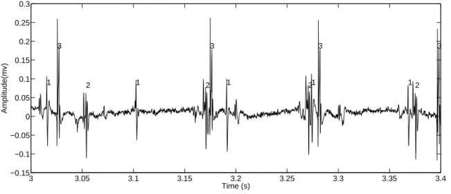
WA, USA) made of Teflon coated stainless steel with a diameter of 0.05 mm. The numbers denote indexes of MU. . . 23 2.6 iEMG signal decomposition[46, 47]: α MNs discharge successively in the spinal cord, then

sending APs to related muscle fibers to formulate the MUAP trains. The summation of MUAP trans, named ’Raw EMG signal’ in the figure, is detected by the needle electrode or wire electrode. The EMG signal is decomposed in the form of several individual MUAP trains corresponding to each active MU discharge. . . 24 2.7 Several similar segments of iEMG signal and the signals filtered by the 1st order and the

2nd order low-pass differentiating filter [53]. Differences between MUAPs were highlighted. 25 2.8 The multi-scale model of movement generation [86]. From left to right: P activation

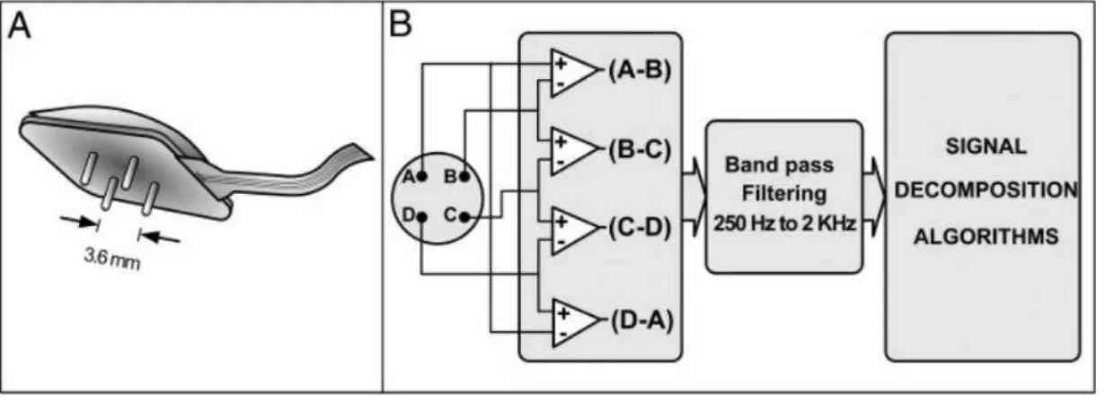
prim-itives are shared by N motor neuron pools (P < N ). Each MN pool receives the linear combination of the P activation primitives as input and transforms this input into spike trains that drive the innervated muscle (thus, the scheme presents N muscles). The N mus-cles contribute to M (M > N ) EMG channels by the trains of MUAPs. . . 29 2.9 A: The quadrifilar needle sensor with larger dimensions containing the 4 pins that detect the

sEMG signals. B: Differential combinations that produce 4 channels of sEMG signals. . . 31 2.10 A: The five-pin surface EMG sensor attached above the First Dorsal Interosseous muscle in

the hand. B: Top and bottom views of the sensor. The four pins on the corner of a square are spaced 3.6 mm apart. . . 32

2.11 The development of language GPU [96]: In the early 2000s, we had to write the applica-tion in shading language. Latter, several academic and third-party languages that abstracted away the graphics appeared. Since 2007, following the step of Nvidia, all GPU manufac-tories launched eventually the GPUs programmable in common program language for the general-purposed computation. . . 32

3.1 The linear model of iEMG signal: The spike train, denoted by Ui[n], is filtered by the corresponding impulse response hi. We obtain the MUAP trains. The summation of the active MUAP trains is the iEMG signal, represented by Y [n] in the figure. . . 36 3.2 Illustration of the relationship between the spike train U [n] and corresponding sawtooth

sequence T [n]; Illustration of MU deactivation/activation events. Time between subsequent spikes was shortened for illustration purposes; in reality, it comprises hundreds of time instants. Moreover, ∆ represent the length of inter-spike interval and N is its index. . . 37 3.3 Example of the discrete Weibull distribution type I with different parameters . . . 40 3.4 Hidden Markov model . . . 41

4.1 Inter-spike law parameters estimation: The first line is the given spike train U [n]; The second line is the estimated location parameter sequence of the discrete Weibull distribution type I; The third line is the estimated concentration one; The forth line is the firing rate. The red horizontal straight line denotes the real value, while the black oscillating line represents the estimated value. . . 45 4.2 Interpretation of F [n]: Red and blue dashed lines represent respectively two MUAP

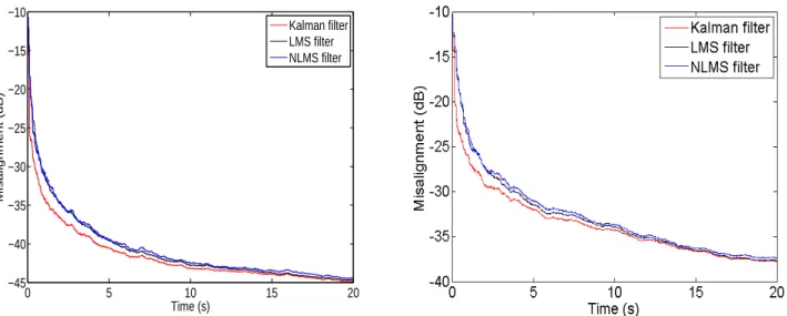
wave-forms. Part of them is superimposed (from n = 10 to n = 21). Black line is the simulated iEMG signal, which is the temporal summation of the two MUAP waveforms. If n < 5 or n ≥ 26, F [n] is a empty set; If 5 ≤ n < 10, F [n] = {1}; If 10 ≤ n < 21, F [n] = {1, 2}; If 21 ≤ n < 26, F [n] = {2}. . . 48 4.3 Comparison of MUAP shapes estimation using three different filters: Kalman filter, LMS

filter and NLMS filter. SNR=20 dB (left); SNR=10 dB (right). Misalignment (in dB) is defined as 20 log₁₀(kH[n]− ˆH

|n Snk2

kH[n]k2 ). . . 49

5.1 Example of iEMG segmentation. Segments are detected using certain threshold and shifted in time to the left by lpd due to the use of future samples. Bifurcations containing impulses are forbidden while Z[n] = 0. . . 56 5.2 Two close cases of MUAP superposition: (a) - exact superposition of two spikes, a case

considered rare and thus excluded from the search; (b) - a close superposition case (∆t denotes the sampling period). . . 57 5.3 The CUDA concept of a grid of blocks [96]. Each block consists of a set of threads that

can communicate and cooperate. Each thread uses its block index in combination with its thread index to identify its position in the global grid. . . 59 5.4 Concurrency example: There are five concurrency examples: 1. Serial execution. 2.

Con-currency execution between a kernel function and the memory copy from device to host. 3. Concurrency execution between a kernel function and two types of memory copies (DH: from device to host and HD: from host to device). 4. Concurrency execution of a kernel function, two types of memory copies and CPU. 5. Concurrency execution of three kernel functions, two types of memory copies and CPU. . . 60 5.5 Two sets of operations of the shared-address-space parallel formulation of quick sort [119] 61 5.6 Bitonic sorting of a sequence with 16 elements [119] (a) The sequence is converted three

times to a bitonic sequence; (b) A bitonic sequence is sorted to a monotonically increasing sequence. . . 62 5.7 Parallel structure of iEMG signal decomposition algorithm . . . 64

6.1 Differentiation (a) The iEMG signal before differentiation; (b) The iEMG signal after dif-ferentiation. . . 68 6.2 MUAP waveforms clipping (a) MUAP waveforms before clipping; (b) MUAP waveforms

after clipping . . . 68 6.3 Acquisition of experimental signals from the abductor digiti minimi muscle . . . 69

7.1 Comparison of automatic decomposition (crosses, ’x’) and actual results (points, ’.’) in the upper panel and the simulated signal with 10 MUs in the lower panel. . . 72 7.2 An extraction of the simulated signal decomposition shown in figure 7.1; circles ’◦’ and

crosses ’x’ represent respectively the spikes from the reference and automatic decompositions. 72 7.3 Initial MUAP shapes (actual MUAP shapes contaminated by the noise) and their actual

MUAP shapes for the signal presented in Figure 7.1 . . . 73 7.4 Normalised misalignment of estimated MUAP shapes . . . 74 7.5 Firing rates for the simulated iEMG (see figure 7.1): the dashed lines (empirical) represent

the actual firing rates; continuous lines (estimated) represent the firing rates calculated via the estimated parameters of discrete Weibull distribution as described in section 4.3. . . 75 7.6 Comparison of automatic (crosses, ’x’) and reference (points, ’.’) decompositions (upper

panel) and the experimental signal from TA, 30% MVC (lower panel). . . 76 7.7 An extract of the experimental signal decomposition shown in figure 7.6; circles ’◦’ and

crosses ’x’ represent respectively the spikes from the reference and automatic decomposi-tions. . . 76 7.8 Eight MUAP shapes (manually-extracted dictionary) for the signal presented in Figure 7.6,

and a comparison between the 2nd one and the 3rd one. . . 77 7.9 Firing rates for the iEMG from TA set (see figure 7.6): the dashed lines (empirical)

repre-sent the firing rates estimated using reference decomposition; continuous lines (estimated) represent the firing rates calculated via the estimated parameters of discrete Weibull distri-bution as described in section 4.3. . . 78 7.10 Comparison of automatic (crosses, ’x’) and reference (points, ’.’) decompositions (upper

panel) and corresponding experimental signal from ADM, in position 5, corresponding to approximately 45 degrees of abduction (lower panel). . . 79 7.11 An extract of the experimental signal decomposition shown in figure 7.10; circles ’◦’ and

crosses ’x’ represent respectively the spikes from the reference and automatic decomposi-tions. . . 79 7.12 Initial MUAP shapes (manually-extracted dictionary) and their final estimations for the

signal presented in Figure 7.10 . . . 80 7.13 Firing rates of the experimental signal with 7 MUs detected from ADM in the abduction

position ’5’ . . . 81 7.14 Delay of experimental signal (recorded from muscle TA, with 8MUs and 30% MVC)

de-composition with 256 paths . . . 82 7.15 Example of a simulated signal with 10 MUs: The recruitment profile is shown in the upper

1

Introduction

1.1

Project

My work of phD thesis is developed in the group ReV (Robotique Et Vivant) and the group SIMS (Signal, Image et Son) of the laboratory LS2N (Laboratoire des Sciences du Numérique de Nantes). In our team, I am supervised by Mr. Yannick Aoustin and Mr. Eric Le Carpentier, specialists in the robotics and signal processing, researching in the domain of biomedical.

The final objective of our team research is to control precisely the active prosthetic devices for amputees with electromyographic (EMG) signals. The active prosthetic devices that we study is the robotic hand of the laboratory LS2N. It is shown in figure 1.1. The LS2N hand is an underactuated robotic hand, constructed by Alpes Instruments (Grenoble) for LS2N. This robotic hand has an underactuated mechanism, which allows to obtain 15 degree of freedoms (DOFs) by using only six actuators. The underactuation mechanism provides several advantages, such as: low weight, low cost of power, and easy control. When the robotic hand does not contact an object, its fingers move as a one DOF serial chain. When it grasps an object, a particular mechanical system allows its fingers to adapt to the shape of the object, acting similarly to a human hand.

Precise control of the active prosthetic devices for amputees with electromyographic (EMG) signals is a very huge and difficult task. The realisation of this work is divided in three steps:

— Extraction of critical information in the signals of muscle, EMG signals.

— Understanding and quantification of the correlation between muscle signals information and the kinematic coefficient of the movement

— Command of the robotic hand to produce a prediscribed movement.

Due to the time restriction of prosthetic control, the first step and the third step should be executed in a real time manner.

A sequential decomposition algorithm based on a Hidden Markov Model of the EMG, that used Bayesian filtering to estimate the unknown parameters of discharge series of motor units was previously proposed in the laboratory LS2N. This algorithm has successfully decomposed the experimental iEMG signal with four motor units. However, the proposed algorithm requires a high time consuming.

In the work of my phD, we firstly validated the proposed algorithm in a serial structure. We proposed some modifications for the activation process of the recruitment model in Hidden Markov Model and im-plemented two signal pre-processing techniques to improve the performance of the algorithm. Then, we realized a GPU-oriented implementation of this algorithm, as well as the modifications applied to the orig-inal model in order to achieve a real-time performance. Specifically, we proposed a replacement of the

Figure 1.1 – Robotic hand of the laboratory LS2N [1]

originally proposed Kalman filter by a least mean square filter with a significant reduction of computational load. Moreover, we introduced two heuristic-based techniques of branch discarding in order to simplify the problem of optimal spike sequence search. Then, an optimal parallelization of the algorithm is presented, along with details of its implementation on graphics processing unit (GPU). Now, We have achieved the decomposition of 10 experimental iEMG signals acquired from two different muscles, respectively by fine wire electrodes and needle electrodes.

During my phD, Mr. Dario Farina gave us some precious advices for our work and provided us several iEMG signals measured by fine wire electrodes. Moreover, Mr. Clement Huneau and his colleague also offered us some iEMG signals measured by needle electrode. These signals and the ones measured by ourselves were successfully decomposed. Our algorithm was validated on various signals from different laboratories, proving its stability, wide applicability and high efficiency.

1.2

Plan of thesis

The manuscript of thesis is organised as following:

— In the chapter 2, we would like to introduce the background of the research, including the basic anatomic knowledge of motor unit (MU), the physiological model to generate the electromyographic (EMG) signals, the EMG signals acquisition and decomposition. Moreover, the development of the parallel computation will also be presented.

— In the chapter 3, the process of derivation from the linear convolution model of EMG signal to the hidden Markov model (HMM) are illustrated.

— In the chapter 4, the Bayes filter is applied to decompose the iEMG signal. It jointly estimate the action potential of MU (MUAP), the firing statistics parameters and the spike trains.

— In the chapter 5, we implement the decomposition algorithm into the parallel computation in order to realise the real-time decomposition. Some heuristic measure are also given in this chapter. — Chapters 6 and 7 present some methods to pre-process the signal, the simulated and experimental

signals, and their results of decomposition evaluated in terms of the complexity, the performance and the speed.

1.3

Table of notations

Table 1.1 – Main notations Y The iEMG signal

Ω The set of indexes of all motor units A The set of indexes of active motor units h Impulse response

U Spike trains

W Noise

H The vector of motor unit action potentials shapes `IR The maximum motor unit action potentials length

T The sawtooth sequences S The activation scenario ∆ The inter-spike interval

Θ = [t0, β] The vector containing discrete Weibull distribution parameters: the location parameter and the concentration parameter

tR The shifting parameter of discrete Weibull distribution, that is the refractory period tI The maximum active time without spike in the recruitment model

λ The activation probability in the recruitment model npath The number of kept scenarios (paths)

τ The active time index in the inter-spike law parameters estimation vSn The variance of innovation in the impulse response estimation

V The variance of noise ˜

v The ratio of the variance of innovation to the variance of noise m∆ The expectation of inter-spike interval

Z The segmentation sequence Sup The superposition percentage E(.) Expectation

Pr(.) Probability w.p. with probability

Y [n] The iEMG signal at time index n

Yn The vector containing the signal from time index 1 to n |n _{Given Y}n

Pr(T [n] = t[n]) The probability of the sawtooth sequences at time index n being equal to a value t[n]. For all elements of the state vector, the uppercase symbols denote random variables, while the lowercase ones stand for their values.

2

Research Background

2.1

Introduction

Our research focuses on the on-line decomposition of EMG signals in the parallel computation. There-fore, in this chapter, we will introduce the background knowledge related to EMG signals decomposition and parallel computation. The first section shows a basic introduction of EMG signals containing the anatomical characteristics of MU which reveals the anatomical relations between motor neuron (MN) and the muscle fibers that it innervates, and the physiological model of EMG signals which describes the physi-ological procedure of generating EMG signals. In the second section, we present EMG signals decomposi-tion, including the various protocols of EMG signals acquisition and several EMG decomposition methods corresponding to them proposed in recent years, in the both off-line and on-line manners. Finally, we will make a review of the development of the parallel computation in Graphics Processing Unit (GPU).

2.2

Electromyographic signals

The movement of humans is the kinematic manifestation of the muscle activities, while the EMG signal is the electrical expression of skeletal muscle fibers during a muscle contraction. They are controlled by the active motor unit (MU) populations, which are the smallest voluntary units in a movement. Each MU comprises two components: the motor neuron (MN) and the muscle fibers that its axon innervates, referred as to the muscle unit.

2.2.1

Physiological model of EMG signal

Human movement is controlled by the activity of cells in neural system, which is composed of the central (CNS) and peripheral (PNS) nervous system. The CNS consists of two major structures, the brain and the spinal cord, which is in charge of integrating information it receives, coordinating and influencing the activity of all parts of the bodies. The brain acting as the major processing unit of the nervous system receives sensory information and command body to make reactions. The spinal cord is not only the bridge between the brain and PNS, but also can accomplish some basic reflex.

The PNS consisting of the nerves and ganglia outside the brain and spinal cord, including the nerve roots, dorsal root ganglia, brachial and lumbosacral plexuses, and peripheral nerves, connects the CNS to other parts of body. Complex peripheral nerves are two-way conduits: Efferent motor information travels from the spinal cord to the muscles, while afferent sensory information travels from the periphery to the

spinal cord. Efferent motor signals travel from the anterior horn cells (α MNs), which are lower MNs under the control of the corticospinal tracts, into peripheral nerves by way of ventral roots, finally reaching the innervated muscle units. Figure 2.1 shows different positions of spinal cord controlling various type of muscles. Compared to the direct measure in the efferent peripheral nerve fibers, the muscle signals as a result of the neural informations spatially spreading from the PNS, have a relatively small number of physiological sources per unit volume and still reveals the same level information on the neural activities.

Figure 2.1 – Central nervous system and the functions of spinal nerves [2]

Although, due to the high complexity of neural systems, the mechanism of movement manipulation are still not completely understood. The EMG signal, as the electrical manifestation of muscle activities, reflects the activity of α MNs in the spinal cord via the peripheral nerves conduction, thus offers us the probability to exploit the neuromuscular system.

The CNS takes charge of recruiting MNs in the spinal cord, in the order of from the smallest to the biggest MU [3], based on the size of the load. The MUs are normally divided into four categories [4] based on their physiological properties: The first three types of MU: fast fatigable (FF), fast intermediate (FI)

and fast fatigue resistant (FR), are all recruited in the movement with fast speed, but with different levels of force. The lower level force is related to the higher resistance of fatigue. The forth type of MU, slow oxidative (SO), recruited during the slow contraction with low force shows a extremely high resistance of fatigue.

Figure 2.2 – Anatomical characteristics fo MU: MNs that innervate the individual muscle are termed motor nucleus or motor neuron pool and cluster in either the anterior (ventral) horn of the spinal cord. Every MN innervates several muscle fibers. The muscle fibers of a muscle unit intermingle with other muscle units, but do not extend to other muscles nearby. (Copyright c 2001 Benjamin Cummings, an imprint of Addison Wesley Longman, Inc.)

A MU consists of an α MN in the spinal cord and the muscle fibers it innervates. Once a MU receives the order from the higher level neural system, its α MN immediately discharges, sending action potentials (AP) propagating along its axon until reaching the neuromuscular junction where they activate sodium channels of muscle cell membrane. Latter provokes a muscle cell’s action potential which propagates along the fiber causing its contraction. The innervating process is illustrated in figure 2.2.

Since a α MN cannot discharge all the time, its successive discharges and equilibrias formulate the sequence of action potentials, usually referred as the spike train. Intervals between discharges are under several physiological constrains. Firstly, the discharge patten (firing patten) of an α MN, whose frequence is termed firing rate, exhibits a specific rhythm and regularity, especially during static contractions, thus can be described by the statistic law. Secondly, intervals between discharges are usually not shorter than a certain duration called refractory period, which is in the order of 30 ms [5, 6, 7].

In a MU, the resulting AP discharged by α MN propagates along the membrane of a muscle fiber can be acknowledged as a temporally charging voltage, termed muscle fiber potential [8]. These muscle fiber potentials belonging to the same MU is not time aligned owing to the different location of end-plates. The spatial and temporal summation of these muscle fiber potentials in a MU is called motor unit action potential (MUAP). In order to maintain the muscle contraction force, α MNs discharge repetitively and generate the MUAP trains, where every MUAP is positioned at times of its α MN discharge. A detected EMG signal is the algebraic summation of these generated MUAP trains and the background interference containing the instrument noise and artifacts.

2.2.2

Anatomy of motor unit

MNs that innervate the individual muscle are termed motor nucleus or motor neuron pool and cluster in either the anterior (ventral) horn of the spinal cord or the brain stem [9, 10], as illustrated in figure 2.2. Motor nucleus of proximal muscles are located more ventral and lateral than those of distal muscles in the transverse section of spinal cord, and motor nucleus of anterior muscle are more lateral than those of posterior muscles [11].

The number of MNs in a motor nucleus, the same as the number of MUs that innervate a muscle, ranges from a few tens to several hundred, which is difficult to calculate due to the limitation of available methods. One of the methods is to retrograde transport of horseradish peroxidase (HRP) either by injection into a target muscle or by exposing the cut nerve to the tracer [12], whose difficulty is to deliver sufficient HRP to the target muscle without involving muscles nearby. Another method is human cadavers dissection, which is limited by the assumption: the proportion of large-diameter axons are efferent fibers. Compared to anatomical methods, an electrophysiological method proposed is to measure the amplitude of muscle potentials caused by stimulating the peripheral nerves [13]. The estimates of electrophysiological method are typically lower than those by anatomical methods.

The muscle unit comprises several muscle fibers. The average innervation number, defined as the num-ber of muscle finum-bers innervated by a single MN, ranges from five to thousand [14, 15]. This average de-pends on the size of different muscles. Moreover, the innervation number varies within a muscle, with low-threshold MUs containing lower values [16]. Due to the high correlation between the innervation num-ber and maximal force of target muscle, the range of innervation numnum-ber in a muscle can be estimated by the force [16].

The muscle fibers of a muscle unit occupy a sub-volume of the muscle [17] and intermingle with other muscle units but do not extend to other muscles nearby [18], as depicted in figure 2.2. Some experiments, such as [19, 20], prove that each muscle unit takes only little fraction of the muscle. Therefore, an interesting issue is the transmission force from the contractile proteins of muscles units to the skeleton modified by the connective issue structures. Since muscle units innervated by different MNs are located in different discrete compartments in a muscle, the muscle can be divided into several distinct regions based on different physiological functions [21]. However, subsequent work demonstrates the properties of human MUs are distributed continuously within a motor nucleus [22, 23] and are not divided into distinct groups. Normally, the types of MUs are distinguished with respect to the threshold of force.

2.3

EMG signals decomposition

As depicted in the physiological model, the EMG signal reflects the activity of α MN, thus providing us an insight view of the neural system. Informations regarding MUAP waveforms and MU firing patterns ex-tracted from EMG signals during muscle contractions are widely used in the different domains, for example: MUAP waveforms are used in the diagnosis of neuromuscular disorders [24, 25, 26] and in the estimation of muscle architecture [27]; MU firing patterns are applied for the investigation of central strategies for motor control [28, 29] as well as for creating human-machine interfaces [30, 31, 32]. Therefore, the identification of individual MN spike trains from the EMG, termed EMG decomposition [33] is an indispensable issue. In

recent decades, a great mass of algorithms in a manual, semi-automatic or automatic ways were proposed to resolve this problem. We will talk about them in the following parts of this section.

2.3.1

EMG signals acquisition

Figure 2.3 – High-density sEMG recordings from a human hand muscle [34]. (A)sEMG signals recorded with an electrode array (5 columns × 13 rows) placed over the abductor pollicis brevis muscle of a healthy man as he sustained an isometric contraction at 10% of the maximal voluntary contraction force. (B) Distribution of multichannel sEMG amplitude at the instant indicated by the red dots and vertical lines in A. (C) Eight MUAPs detected by the array electrodes.

The beginning step of the EMG signals decomposition is the EMG signals acquisition. An improper EMG signal cannot be decomposed accurately even by the most efficient decomposition method. The type and position of electrodes, the contraction level and the fatigue state of the muscle, as well as the artifacts controlling by the operator, affect the decomposability of a detected signal.

EMG signals are recorded using either surface (surface EMG, sEMG) or intramuscular electrodes (in-tramuscular EMG, iEMG). sEMG electrodes are usually placed on the skin overlying the target muscle. It has several advantages, such as: non invasive, convenient to use and non pain felling for the subject. How-ever, the volume conductor of the overlying muscles and other subcutaneous tissues acting as a low-pass

filter whose selectivity depends on the distance between the electrodes and the source limits the bandwidth of sEMG signals. Moreover, due to the large pick-up area of surface electrode, it is influenced also by the interference of adjacent muscles (cross-talk) makes the decomposition more challenging. Thus, compared to the iEMG ones, the sEMG signals detect the activity containing more MUs, which overlap mutually and cause cancellations of amplitude, formulating a highly complex signal pattern that is difficult to interpret. In most of sEMG decomposition algorithms [35, 36, 37, 38, 39] proposed recently, the sEMG signal acqui-sition is always executed in a fashion of multiple electrodes arranged in a two-dimensional arrays in order to obtain the spatial variability of MUAP shapes.

Figure 2.4 – Different types of needle electrodes [40]:(a)Single fiber electrode (b) Concentric electrode (c) Monopolar electrode (d) Macro electrode

Intramuscular electrodes are more spatially selective [41] than the surface ones. The indwelling elec-trodes inserted directly into a muscle are able to detect the EMG activity in deep area. An iEMG signal is usually produced by a limited number of MUs, with MUAPs distinct from the noise, although superim-posed with each other in time. However, some disadvantages are associated with it [40]. Firstly, owing to the invasive property, the iEMG signals acquisition always requires the human interactive. The inserted needle damages some muscle fibers nearby and causes a small local oedema. Sometimes, it could cause unintentional damage of important structures. Secondly, the iEMG signals record only a small number of MUs closed to the detection site. Thirdly, due to the small volume detected by iEMG electrodes, it is diffi-cult to replace the electrode in the same position, thus to repeat the experimentation before. Despite theses limitations, iEMG signals decomposition is attractive for a great many researchers.

Due to the high selectivity of the iEMG signals, many researchers prefer it to offer an accurate de-composition. Therefore, different needles were proposed to measure the iEMG signal to adapt to specific algorithms for information extraction. As one of the earliest proposed needle electrodes, the concentric needle electrode [42] detects signals between the tip of a wire insulated in the cannula and the cannula.

3 3.05 3.1 3.15 3.2 3.25 3.3 3.35 3.4 −0.15 −0.1 −0.05 0 0.05 0.1 0.15 0.2 0.25 0.3 1 ₂ 1 ₂ 1 ₂1 1₂ 3 3 3 3 Amplitude(mv) Time (s)

Figure 2.5 – Example of iEMG signal was acquired using 25G wire electrodes (A-M Systems, Carlsborg, WA, USA) made of Teflon coated stainless steel with a diameter of 0.05 mm. The numbers denote indexes of MU.

To fulfil different requirements, some others needle were proposed in recent years, such as: single fiber electrode and monopolar electrode, as figure 2.4 shown. Sometimes, if informations related to MU size or fiber spatial distribution are required, the macro electrode records a more broadly detected signals from the cannula surface.

During the iEMG signal acquisition, slight movements of the centric needle are often inevitable, causing not only the pain of the subject but also the modification of MUAP shapes in the detected signals. To overcome this limitation, wire electrodes [43] were proposed, which are usually appreciated in the long period recording or the recording of movement. The wire is placed in the cannula of a needle and bent at the tip. The needle is inserted into the muscle then removed to make the wire stay in the muscle. Once placed into muscle, its position cannot be adjusted. The wire electrode allows the strong contractions without the discomfort feeling. It shows a stabler property versus the needle ones. An example of iEMG signal aquaired using 25G wire electrodes (A-M Systems, Carlsborg, WA, USA) made of Teflon coated stainless steel with diameter of 0.05 mm, is shown in figure 2.5. Wire electrodes are difficult to arranged in geometrical sites in a single system to extract the spatial informations of the detected muscle. Then, longitudinal intra-fascicular electrodes (LIFE) [44] were proposed to resolve this problem, which are fine wire electrodes implemented into peripheral nerves. The recent generation of this system consists in thin-film LIFE [45]. These systems allow the multi-channel iEMG signal acquisition in a single insertion and the repeat experimentations in the same detected site.

2.3.2

iEMG signals decomposition

As depicted in figure 2.6, α MNs discharge successively in the spinal cord, then sending APs to related muscle fibers to formulate the MUAP trains. The summation of MUAP trans, named ’Raw EMG signal’ in the figure, is detected by a needle electrode or a wire electrode. The EMG signal is decomposed in the form of several individual MUAP trains corresponding to each active MU discharge. The individual MUAP train is the convolution of MUAP shapes of each MU and the spike trains, which is the discharge patten of α MN in subsection 2.2.1. In the rest of this subsection, we will present various decomposition algorithms, which were proposed to realise the complete or incomplete decomposition of iEMG signals.

The procedures for iEMG signal decomposition have been progressively improved from methods strongly based on the manual intervention of an operator [48, 49, 50] to semi-automatic and then fully automatic

Figure 2.6 – iEMG signal decomposition[46, 47]: α MNs discharge successively in the spinal cord, then sending APs to related muscle fibers to formulate the MUAP trains. The summation of MUAP trans, named ’Raw EMG signal’ in the figure, is detected by the needle electrode or wire electrode. The EMG signal is decomposed in the form of several individual MUAP trains corresponding to each active MU discharge.

methods. The initial manual methods rely on the visual inspection of similar MUAP shapes matching in an EMG signal shown on an oscilloscope or plotted on a grid paper. These methods are time consuming and cannot achieve an ideal decomposition, especially in the case of a great many superposed MUAP shapes in the signal. And the quality of decomposition always depends on the experience of operators. With respect to the manual methods, semi-automatic and fully automatic methods are more powerful. Some of tech-niques are used in both of them. In most of semi-automatic and fully automatic algorithms, the process of MUAP trains identification is implemented by pattern recognition techniques. More recently, blind source separation approaches have been proposed to decompose multi-channel iEMG signals [31, 51], acquired by thin-film LIFE. This kind of approach is appreciated as they are minimally influenced by the MUAP overlap rate.

Pattern recognition methods

Firstly, we present the outline of semi-automatic and fully automatic algorithms based on pattern recog-nition techniques. These decomposition procedures normally includ the following steps [52] after the ac-quisition of signals:

— Signal preprocessing

— Signal segmentation: MUAP detection — Feature extraction

— Clustering and supervised classification of detected MUAP shapes — Superposition resolving

The first step signal preprocessing is to decrease the influence of background noise and low frequency information, including some small dimension MUAPs taken as noise, by filtering the signal. Moreover, it is also applied to sharpen MUAP shapes and increase the dissimilarity of MUAP shapes, as the example illustrated in figure 2.7. Thus, signal preprocessing improves the MUAP detection and classification. Band-pass filters or low-Band-pass differentiating filters [53], which are easy to implement and fast to execute, are commonly used in this step. These filters suppress the baseline of noise but without attenuating greatly the MUAP amplitude, which simplifies the signal segmentation. Besides the two filters, some others complex wavelets [54, 55] and empirical methods [56] coasting more execution time were applied to remove the noise in the signal. They may work better than the previous two filters. However, their performances depend largely on some pre-defined parameters by users, such as the de-noising threshold or the mother wavelet of the wavelet-based methods.

Figure 2.7 – Several similar segments of iEMG signal and the signals filtered by the 1st order and the 2nd order low-pass differentiating filter [53]. Differences between MUAPs were highlighted.

The objective of the second step, signal segmentation, is to separate the noise and the single or super-imposed MUAP segments, thus to detect all activities of MUs. Normally, a threshold crossing the whole iEMG signal is profited. The local peaks of filtered signals exceeding this threshold are taken as the can-didate segmentation positions. A window is used to center these peaks and extract the signals nearby to formulate MUAP segmentations. The threshold can be artificially pre-defined as a positive value [46, 47], or can be calculated based on the characteristic of the filtered iEMG signal [53, 57, 58, 59, 60], such as the maximum absolute value, the mean of absolute value and the standard deviation of signal. The length of window can be variable [55, 57], which is adjusted regarding to the duration of MUAPs, or constant, normally chosen as 2.5 ms [61, 62] or 6 ms [58, 59]. The shorter window length can simplify the procedure of clustering and classification, but cause multi-detection of some long MUAP segmentations and the extra fusion procedure, while the longer window length can keep more information of MUAP segmentation, but increase the decomposition time.

In the step of feature extraction, a feature vector is composed of a number of features extracted from MUAP segmentations obtained in the previous step. The dimension of feature vector is typically not too large to require a large mass of computation resource, nor too small to accurately classify these MUAP segmentations. Ideally, the feature vector contains a few number of uncorrelated features which desire less time to calculate and are sensitive to discriminate MUAP segmentations belonging to various MU classes. Moreover, these features should decrease the effect of MUAP superposition and have a tolerance of the variability of MUAP shapes. Until now, different features were extracted to represent the detected MUAPs, improve the accurancy of decomposition and reduce the time execution. These features can be principally divided into time-domain, frequency-domain, wavelet domain features, such as: first and second derivative time samples [46, 47, 61, 62], variance [63], mean frequence and mean power [64], total power and variance of central frequence [65], power spectrum and Fourier transform coefficient [53], and wave coefficient [55, 66]. In addition, besides different features in time-domain, frequency-domain or wavelet domain, some morphological features are involved in the decomposition algorithm because they are easier to calculate. Morphological features are briefly presented in table 2.1.

Table 2.1 – Morphological features of MUAP shapes

Name Description

Duration The time between the onset and the termination of an MUAP. Peak-to-peak amplitude The difference from the maximal to the minimal peak

Number of phases The number of baseline crossing plus 1

Number of turns A turn is a positive or negative peak that is separated from a previous and a following peak of opposite polarity.

MUAP area The integration of the rectified MUAP over its duration. Maximum positive (or negative)

peak amplitude

the maximum positive (or negative) peak in the MUAP segmen-tation

Both of clustering and supervised classification is the task for partitioning the MUAP segmentations represented by the feature vector into various different MU classes according to their similarities and corre-lations. Generally, we define clustering as the first phase of supervised classification. The several beginning seconds of signal are usually taken for the clustering phase as the training sample of supervised classifi-cation. Although, in some algorithm, there is only clustering, no supervised classificlassifi-cation. Regarding to the aspect of initial condition, no prior knowledge is offered in the clustering, while some informations obtained in the clustering, which is typically the pre-classified MUAP containing the number of MUAP and basic features of MUAP shapes, are initially provided for the supervised classification.

For the clustering, the main difficulty is finding the optimum number of clustering with the interference of MUAP superposition. Some popular clustering algorithms are applied in this phase: K-means, different types of support vector machine, fuzzy c-means and the hierarchical algorithm. Moreover, some decompo-sition methods combines the clustering with a mathematical model in order to find the spike train of each MU. [67] use the combination of MUAP shapes and MU firing patten provided by a spike train constrained Viterbi algorithm to find the best combination for each MUAP segmentation.

In the supervised classification phase, the variability of MUAP shapes caused by the movement of needle inserted in the muscle, by the neuromuscular jitter or by the fatigue of muscle, can increase a large number of missed classification error, thus reduce the decomposition accuracy. To resolve this problem, the firing rate pattern of MU is often taken as the regularity restriction for the classification. It is used passively in the way of testing the regularity to fill the gap or eliminate the peak of MUAP trains, or actively with the MUAP shapes to determinate the certainty in assigning a MUAP into its MUAP trains. However, two disadvantages limit the implementation of firing rate pattern. The first one is the double discharge of MU (firing twice closely in time). Second, a relative stable stochastic process of firing rate patten is normally in the case of slow change of force. In the case of fast change of force, the firing rates are largely time-varying and difficult to trace.

EMG signal decomposition employs several classification techniques in a variety of algorithms. The maximum a posterior classifier is applied in the algorithm, named Pricision Decomposition 1 (PD1), of [46, 47]. This system was able to decompose iEMG signal less than 8 MUs with an accurancy of 60 to 70% in an automatic mode. And it provides a way of human interaction to reach higher accuracy. To improve the performance of PD1, the artificial intelligence-based maximum a posteriori classifier is used in [68, 69, 70], termed Pricision Decomposition 2 (PD2). PD2 set automatically the parameters in PD1 based on the statistic characters of iEMG signal with a knowledge-based artificial intelligence framework. Moreover, with respect to PD1, this system can resolve complex superimposition. Both PD1 and PD2 use multi-channel iEMG signals detected by the special quadrifilar needle or wire sensor. Pricision Decomposi-tion 3 (PD3) was proposed in [71] but for sEMG signal, which will be presented in subsecDecomposi-tion 2.3.3. Some algorithms prefer the fuzzy logic-based classifiers. [61] use a fuzzy k-nearest neighbor classifier for the MUAPs supervised classification after the initialisation clustering phase. Certainty-based classifiers [72], which combine MUAP shapes and MU firing rate patten, make an evaluation of certainty to assign a MUAP to one of MU classes. It classifies the MUAP to a class if the largest certainty of related class is greater than the certainty assignment threshold. Otherwise, this MUAP segmentation is unassigned and taken as the su-perposition. Moreover, multiple classifier systems [73, 74] were built to achieve a higher accuracy. [73] was composed of adaptive certainty-based classifier, adaptive fuzzy k-nearest neighbor classifier and adaptive matched template filter classifier. This classifier fusion system showed a better classification performance, especially regarding to eliminate classification errors.

Two or more different MUs fire simultaneously or within a sufficient short time less than the length of MUAP shapes, which is the superposition of MUAPs. The peel-off method [46, 75, 58, 76] based on MUAP shapes matching is the simplest approach to resolve the superposition problem. By measuring the similarity form between the superimposed MUAP segmentation and the MUAP template, we select the most probable template and then the superimposed MUAP segmentation subtract this template. The resulting new form repeats this process until reaches the stop criterion. Another method is the modelling-based approach [77, 78] which perform better than the peel-off method but is more time-consuming. The goal of this method is to find a sum of convolution between MUAP shapes and the firing time to minimize the criterion:

e = kM U APSU P − X

i

hi∗ Uik2 (2.1)

Where M U APSU P is the superimposed MUAPs, h is the MUAP shapes, U is the spike train, i denotes the index of MU and e represents their square of difference. The information of MU firing rate patten is sometimes taken as a reference in the superposition analysis.

When we complete the iEMG decomposition, the spike train or MUAP trains of each MU is identified. Estimations of MUAP templates and MU firing patten statistics are the final step for the various following applications. During the process of MUAP shapes estimation, several methods, such as mean [79, 80], median [80] and interference cancelling averaging technique [53], were applied to reduce the influence of the noise and MUAP shapes of other MUs because of improper classifications. If the number of MUAP segmentations classified to a train is large enough, mean estimation shows a good performance and provide a better SNR than other estimation. Otherwise, if the number is small, the median or median trimmed mean averaging estimations are preferred because they can reduce the interference of MUAP shapes of other MUs because of improper classifications. For the estimation of MU firing patten statistics parameters, once the spike train is offered, the firing rates can be calculated by the number of firing spikes in a second.

These algorithm presented before are typically evaluated by the MUAP shapes estimation and the accu-racy spike trains, which corresponds to the miss assignments and over assignments of spikes. However, in these algorithms, their resolved problems (with or without MUAP shapes superposition), their validations on simulated and experimental signals with different durations, number of MUs, percentage of superpo-sition, similarities of MUAP shapes and ratios of signal to noise (SNR), and their different assessment indexes make the comparision of performance evaluations difficult. There is not a well-known conventional evaluation criterion applied in all papers, although a few practical assessment indexes were proposed in

[81].

Most of the algorithms presented are fully automatic methods, except PD1 [46, 47] and EMGlab [79] which are semi-automatic and need human intervention, especially EMGlab, offering an Graphical User Interface for users. And we notice that almost all pattern recognition methods decompose iEMG signal in a non-sequential manner, which cannot carry out the real-time decomposition.

Blind source separation approaches

Except these pattern recognition methods, blind source separation approaches [31, 51] applied for the iEMG decomposition were proposed in the last few years. The most famous method Convolution Ker-nal Compensation (CKC) of [35], by wihch a convolution matrix comprising the information of MUAP shapes is compensated, designed for the decomposition of multi-channel sEMG signals can be also used for multi-channel iEMG signals decomposition. We will present it in subsection 2.3.3. In [31], an extended measurements was used in the formula 2.2 the same as the extended convolution model proposed in [35], in order to describe the conditions under which the assumptions of the convolutive blind separation model are satisfied. Then, it proposed an approach of convolutive sphering of the observations which is based on [82], followed by an iterative extraction of the sources. In [51], another blind source separation approache is presented. The cyclostationary properties of MUAP trains are used to decompose the iEMG signals.

With respect to the pattern recognition algorithm, blind source separation approaches are generally applied for the multi-channels iEMG signals and usually have a relative high resistance for the interference of MUAP shapes variability. Due to the large amount of the multi-channels iEMG signals, they need more time to process signals. Moreover, their performance strongly depends on the number of available channels [51]

On-line decomposition method analysis

In [83], a real-time decomposition method for the signal channel iEMG signal based on the pattern recognition techniques was proposed. This method is composed of on-line single-pass density-based clus-tering and adaptive classification of bivariate features containing the root mean square and the difference absolute standard deviation, using the concept of potential measure. The superposition problem which is the most complex and time-consuming problem in the decomposition was not taken into consideration in this paper. This algorithm achieves a high accuracy in the classification of the non-supervised MUAP seg-mentations with a speed of 200 ms signal decomposed within 21 to 97 ms. However, it is limited for the movement with high maximal voluntary contraction force (MVC), in which the iEMG signals with more supervised MUAPs segmentations is generated.

In [84, 85], a new algorithm that allows a full decomposition of single-channel iEMG signals produced during dynamic contractions at moderate force levels was proposed. The algorithm is based on a Markov model of the iEMG, which takes into account the varying number of active MUs and the regularity of their spike trains. Joint superposition resolution, MUAPs shape updates and firing statistics estimation are achieved by applying the Bayes filtering. Sliding window approach made the algorithm adaptive to variations of contraction forces and the variability of MUAP shapes.

Although this algorithm needs long time to complete the decomposition, it shows a potential to realise the on-line decomposition. The sequential decomposition way in this algorithm is a necessary condition for the real-time decomposition. Besides, because of its parallel structure, this algorithm can be efficiently accelerated by parallel computation implementation in GPU.

2.3.3

sEMG signals decomposition

Similar to the iEMG signal, sEMG signal is also a measure of muscle activities and thus, an output of the MN spike trains, containing the information on both central and peripheral neural mechanisms for movement generation. However, compared to the iEMG signal, sEMG signal has much higher complexity

due to the superimposition of sources of neural informations at different levels and in mixing unknown process, as shown in figure 2.8. Therefore, the extraction of sEMG information which is taken as the source separation focus on different scales [86]. Figure 2.8 shows the multi-scales form left to right. Firstly, sources in the sEMG signal can be viewed as the high-level commands of the coordinated activity of multiple muscles, where the sEMG is interpreted as the complex muscle activation patterns [87, 88]. Secondly, at a smaller scale, source is considered as the neural activation to different muscles, where the sEMG is processed to identify the activity of target individual muscle or muscle compartments [89, 90]. At this scale, the great challenge is that the record sEMG is usually the mixture of the activities of many concurrently active muscle compartments and neighbor muscles, termed as EMG crosstalk. Finally, at the individual muscle level, source is taken as the activation of the smallest functional units (MUs), where the sEMG is identified in the form of spike trains of each MU and then, the correlated discharge rates and MUAP shapes are estimated [35, 91]. The decomposition of sEMG at this scale is to extract the information form the α MN to the target muscle and thus, provides a definitive insight into the net output from the CNS and PNS. In the decomposition, since the MUAP shapes vary with respect to many factors, such as the subject anatomy, muscle fatigue and etc, they are usually unknown a priori. Moreover, the volume conductor, defined as the tissue separating the muscle fibers and the recording electrode, works as a low-pass spatial filter, where all the signal collected is low-pass filtered with reference to the distance between the muscle fibers and the electrodes. Despite these restrictions limit the sEMG decomposition, some algorithms were proposed to identify the spike trains of MUs in an efficient and robust way, as it presented in [35, 92, 71, 91].

Figure 2.8 – The multi-scale model of movement generation [86]. From left to right: P activation primitives are shared by N motor neuron pools (P < N ). Each MN pool receives the linear combination of the P activation primitives as input and transforms this input into spike trains that drive the innervated muscle (thus, the scheme presents N muscles). The N muscles contribute to M (M > N ) EMG channels by the trains of MUAPs.

To exploit the spatial variability of the detected MUAPs in the sEMG signal, the surface electrodes are always arranged in to two dimensional arrays on the target muscle. Therefore, the multi-channel sEMG signal recorded in the grid electrodes were modeled as the correlated instantaneuos or convolution data models. In the instantaneuos model, the MUAPs trains recorded in the different locations were assumed to vary only in the amplitude. For the i-th MU recorded in the j-th electrode, we have the formula: MUAPij = gij × MUAPst, where gij is a scalar weight and MUAPst stands for the standard constant MUAP shape of the i-th MU. Different with the instantaneuos model, the convolution model assumed that the discharge timings of each MU, that is, the spike train, were shared in the recording of different electrodes, while the detected MUAP shapes were taken as the mixing process itself. It is evident that the convolution model is much more general, realistic and closer to the physiological MUAP model, exhibiting the spatial variability of MUAP shapes.

Both of the instantaneous model and the convolution model can be modeled by the formula:

EMG(n) = G H ¯s(n) + w(n) (2.2)

where EMG(n) = [EMG1(n), · · · , EMGN M(n)] denotes a vector containing N M channel sEMG signals,

and w(n) is the vector of noise. The vector ¯s(n) = [s1(n), s1(n−1), · · · , s1(n−L), s2(n), · · · , sN R(n), · · · , sN R(n− L)] contains L consecutive samples of R MU spike trains in the N MN pools (motor nucleus). In the case

of instantaneous model, G is a N M × N R matrix comprising the scalar weight of MUAP and H is a block diagonal matrix composed of the N R MUAPs. The formula H is shown:

H =      MUAP1(n) 0 · · · 0 0 MUAP2(n) . .. 0 .. . ... . .. 0 0 0 · · · MUAPN R(n)      (2.3)

In the case of convolution model, the matrix G and H can be modeled by a matrix containing the MUAPs shapes of all MUs recorded in all electrodes:

GH =   

MUAP1,1(n) MUAP1,2(n) · · · MUAP1,N R(n) ..

. ... . .. ...

MUAPN M,1(n) MUAPN M,2(n) · · · MUAPN M,N R(n)  

 (2.4)

Based on the convolution model, some algorithms proposed for the sEMG signals decomposition reveal a good performance, especially the algorithm of Convolution Kernal Compensation (CKC) in [35] based on blind source separation techiniques. The CKC estimator is principally based on the computationally attractive linear minimum mean square (LMMSE) estimator, which is Bayesian optimal for linear mixing system, and can estimate the spike trains of individual MU without the calculation of the mixing matrix GH. The LMMSE estimator assumes that the mean of the first two moments of the source signals (spike trains) and their cross-correlation with the observation signals are known in priori. Some supervised ways involving the human intervention were proposed before to overcome this problem. In the CKC estimator, the mixing matrix GH is compensated by the calculating the square of Mahalanobis distance of the extending vector ¯s(t) and thus, find the indexes and time instant of MUs arising the spike in a segmentation of observed signal. Then, according to the analyze of the superposition MUAPs probability, some moments of source signals are estimated. Thus, the condition a priori of LMMSE is fulfilled in this automatic manner in the CKC estimator. The performance of this algorithm shows a high accuracy and robustness. It allows weak correlations between MUs. Moreover, there is no parameter to determine a priori in the decomposition.

Some ameliorations and validations of CKC estimator, such as identification of MU behavior in patho-logical tremor, were proposed in [36, 37, 38, 39]. An algorithm proposed in [93] combining the the K-mean clustering method and a modified CKC method for multichannel sEMG decomposition were validate in the signals more than 10 MUs with a high accuracy. Moreover, a real-time decomposition algorithm based

Figure 2.9 – A: The quadrifilar needle sensor with larger dimensions containing the 4 pins that detect the sEMG signals. B: Differential combinations that produce 4 channels of sEMG signals.

on CKC estimator is presented in [92]. Compared to the off-line version, the real-time one begins with a 3 s batch processing of sEMG signals and then, a tracking formula implemented in the CKC estimator to realize the recursively estimation. The results of experimental signals decomposition reveal that it is unable to detect some source trains compared to the off-line one and has a poor performance in the beginning of decomposition. In addition, it is evident that the first 3 s signal is not identified in a real-time way. But the decomposition results after 3 s are relatively high coincidence with the off-line estimation.

Besides the series of CKC methods, there are also lots of algorithms, which prefer the pattern recogni-tion techniques similar to the iEMG signal decomposirecogni-tion, but using some special dedicated surface elec-trodes to detect sEMG signals with more discriminating MUAP shapes [71, 91], or making a similar as-sumption [94, 95]. In [71], Precision decomposition 3 (PD3) was proposed for sEMG signal decomposition, while PD1 and PD2 systems were designed for the iEMG. With respect to PD2, PD3 system does not show an evident improvement. Both of them use a knowledge-based artificial intelligence framework to automat-ically decide the parameters based on the processing signals and to resolve the superposition. The greatest difference between them is that there are more differential electrodes in PD3, as depicted in figure 2.9, to offer a specific version of signals. Latter, another special detector was presented in [91], as shown in figure 2.10. This five-pin surface sensor can detect sEMG signals with more discriminating MUAP shapes. Then, a new Precision decomposition system containing two phase PD-IPUS and PD-IGAT was proposed. PD-IPUS is almost the same system as PD3 presented in [71] to identify the MUAP segmentation without significant superposition and update the time-varying variations of MUAP shapes, while PD-IGAT com-prises a MUAP template-matching procedure and an iterative MUAP discrimination analysis to resolve the superposition. As presented in [91], experimental signals detected from five different muscles were decom-posed with average accuracy 92.5% during the isometrical contraction at force level ranging up to 100% MVC, which needed a long processing time.

2.4

Parallel computation with graphics processing unit

In the last few ten years, we have entered to the epoch of GPU computing. The GPU computation taking a relative important place in the field of high performance computing (HPC) is applied in a great number of applications with substantial parallelism to achieve superior efficiency. In this section, we will present simply the development of GPU computing and its basic knowledge.

When we talk about GPU computation, we normally make a comparison with Central Processing Unit (CPU) that is highly optimised to execute orderly a series of operations. One of the important index to

Figure 2.10 – A: The five-pin surface EMG sensor attached above the First Dorsal Interosseous muscle in the hand. B: Top and bottom views of the sensor. The four pins on the corner of a square are spaced 3.6 mm apart.

Figure 2.11 – The development of language GPU [96]: In the early 2000s, we had to write the application in shading language. Latter, several academic and third-party languages that abstracted away the graphics appeared. Since 2007, following the step of Nvidia, all GPU manufactories launched eventually the GPUs programmable in common program language for the general-purposed computation.

evaluate the performance of CPU was its frequency. If we double the frequency of CPU, we double its performance. In a long time, we ameliorated the performance of CPU by increasing its frequency until we hit the ’power wall’. In fact, if you fix the voltage, the power consumption of a CPU is approximately the cube of its frequency (clock rate). When we reach a clock rate at around 4 GHz [97], we cannot cool sufficiently the heat of chip converted from such power. Due to the single-core CPU had reached its ceiling, multi-core CPU was designed to increase performance. Meanwhile, the GPU drew more and more attention due to its massive parallelism.

In the early 2000s, GPU was designed to produce a color for every pixel on the screen using pro-grammable arithmetic units known as pixel shaders. The possessed propro-grammable pipelines, by which the user writes a single thread program to making the GPU draw multiple pixels in parallel, attracted the interest of many researchers to exploit the possibility of using graphics hardware for the general-purposed computa-tion. However, in the graphic program, several disadvantages limit the application of the general-purposed computation in the earlier GPU. First of all, the graphic program must be written in shading language, such as Cg or High-Level Shading language (HLSL) [98]. The users should store their data in graphics textures and execute computations by calling OpenGL or DirectX functions, which was coded with shading language. Thus, before enjoying the massive parallel computation power of GPU, the users should learn the knowledge of computer graphics and shading languages. Secondly, there were serious limitations on how and where the user could write results to memory. Finally, it was impossible to terminate the graphic program when we got an unexpected results. There weren’t any reliable debugging methods.

With the Nvidia GeForce 8800 introduced in 2006, the first unified graphics and computing GPU archi-tecture was programmable in CUDA C with the CUDA parallel computing model, as well as using DX10 and OpenGL. NVIDIA took industry standard C and added a relatively small number of keywords in order to harness some of the special features of the CUDA Architecture. Latter, Tesla T8 C870, as the first GPU computing system programmed in CUDA C with CUDA was launched in 2007. Compared to the earlier GPU, the CUDA architecture comprised an unifed shader pipeline [99], which allows every arithmetic logic unit (ALU) on the chip to be marshalled by a program intending to perform general-purpose computations. These significant milestones in the development of Nvidia GPU technology, as well as the GPU computing, signified that users were no longer required to have any knowledge of the shading language. As shown in figure 2.11, since 2007, following the step of Nvidia, other GPU manufactories released general-purpose languages for the GPU programming [96]. Nowadays, the most popular GPU programming language are NVIDIA CUDA, DirectCompute, and OpenCL. After the first shoot for language C, CUDA as a parallel computing platform and application programming interface (API) model created by Nvidia released the restriction for other programming language, such as: C++, Fortran and Matlab.

There are three major GPU companies: Intel, Nvidia and AMD for the Personal Computer (PC) market today. Intel is the largest one, but focusing on the integrated and low-performance GPU market, while Nvidia and AMD are the major supplier for the high-performance market. In the academic and industrial field, Nvidia has a dominant position due to the community support, despite the GPU of AMD shows the same excellent performance. Therefore, we focus on GPU of Nvidia in the thesis.

There are three series of Nvidia GPU termed respectively Tesla, Quadro and GeForce. Quadro is de-signed for the professional workstation; Tesla is used for the scientific computation; And Geforce aim at the market of gaming. Although some laboratories prefer Geforce to execute the scientific computation due to its low price and high power. The computation stability of Geforce cannot be compared with Tesla. After the first generation of GPU designed specially for General-purpose computing on graphics processing units (GPGPU) [100] with the architecture named Tesla, the same name as the series, Nvidia cooperation developed gradually GPUs with Fermi, Kepler, Maxwell and Pascal architectures for GPUs. With the im-provement of GPU architecture, a huge leap forward in power efficiency is offered and a great many features were developed. The GPU power efficiency reached the level of TFlop of double precision, Where TFlop refers to the capability of a processor to calculate one trillion floating-point operations per second. Vari-ous type of GPU memories containing the register, shared memory, constant memory and global memory breaks the memory wall thus reduce the consummation of memory transition. Multi-streams allow the