Science Arts & Métiers (SAM)
is an open access repository that collects the work of Arts et Métiers Institute of Technology researchers and makes it freely available over the web where possible.
This is an author-deposited version published in: https://sam.ensam.eu
Handle ID: .http://hdl.handle.net/10985/9514
To cite this version :
Mohamed Aziz NASRI, Jose Vicente AGUADO, Amine AMMAR, Elias CUETO, Francisco CHINESTA, Franck MOREL, Camille ROBERT, Saber EL AREM - Separated representation of incremental elastoplastic simulations In: ESAFORM 2015, Autriche, 201504 ESAFORM 2015 -2015
Any correspondence concerning this service should be sent to the repository
Separated representation of incremental elastoplastic simulations
Mohamed Aziz Nasri
1,a, Jose Vicente Aguado
2,b, Amine Ammar
1,c,
Elias Cueto
3,d, Francisco Chinesta
2,e, Franck Morel
1,f, Camille Robert
2,gand Saber Elarem
1,h1LAMPA, ENSAM Angers, France
2GeM Institute, Ecole Centrale de Nantes, Nantes, France 3I3A, Univzersity of Zaragoza, Spain
a[email protected],b[email protected],
c[email protected],d[email protected],e[email protected], f[email protected],g[email protected],h[email protected]
Keywords: Model Order Reduction. Proper Generalized Decomposition. Elastoplasticity.
Abstract. Forming processes usually involve irreversible plastic transformations. The calculation in
that case becomes cumbersome when large parts and processes are considered. Recently Model Order Reduction techniques opened new perspectives for an accurate and fast simulation of mechanical systems, however nonlinear history-dependent behaviors remain still today challenging scenarios for the application of these techniques. In this work we are proposing a quite simple non intrusive strategy able to address such behaviors by coupling a separated representation with a POD-based reduced basis within an incremental elastoplastic formulation.
Introduction
The main difference between viscoplascticity and elastoplasticity is that in elastoplascitity the behavior at each position and time depends on all the previous mechanical history as well as on the present loading. Obviously if the deformation history is given at each position, the elastoplastic behavior law can be easily integrated in order to compute the stress evolution. However such an information is not generally available when proceeding with standard discretization strategies where the solution is computed incrementally.
When using standard incremental discretization techniques we must proceed differently. We as-sume at time tn(time in the sense of loading) the state of the systems perfectly defined, verifying the
equilibrium and the constitutive equations. The mechanical state is given by ϵn, σn, ϵpnand αn, the last
being the internal variable describing the material hardening (accumulated plastic deformation, plastic work, ... ) assumed isotropic without loss of generality.
The equilibrium at time tnwrites in discrete form:
Fint(σn) = Fextn (1)
Now, an increment of load applies due to volume forces or surface tractions, and the problem consists in computing the displacement change ∆un+1 and the associated final state defined by
ϵn+1, σn+1, ϵpn+1 and αn+1. The new state must verify both the equilibrium
Fint(σn+1) = Fextn+1 (2)
and the rate-independent elastoplastic constitutive equations. As the problem is nonlinear we must iterate. We denote by ∆Ukn+1the nodal displacements increment at the loading step tnand the nonlinear
iteration k.
A soon as the nodal displacement increment ∆Uk
n+1 is given, we can compute σn+1k by using an
appropriate return mapping [10] that allows after assembling evaluating the internal contributions
Fint(σk
The displacement increment results from the Newton linearization of Eq. (2) that results in
Fint(σn+1k )− Fextn+1 = Kkn+1∆Uk+1n+1 (3) where in the calculation of the tangent matrix Kk
n+1the return mapping algorithm is considered again.
The possibility of applying a space separated representation for alleviating the complexity of 3D so-lutions is being evaluated.
The main difficulty associated with such an approach is its incremental character that makes dif-ficult the use of model order reduction techniques based on the use of separated representations.
The LATIN method is one exception. The LATIN method, proposed by Pierre Ladeveze in the 80s [8] proceeds by assuming a space-time representation of both the deformation and the stress fields. It consists of two stages. In the first, stresses and strains are calculated in order to verify the constitutive equation, by assuming a certain (a priori arbitrary) relation between both fields, that is: knowning at iteration k (iteration in the nonlinear sense) ϵk(x, t) and σk(x, t), we look for ˆϵk(x, t) and ˆσk(x, t), such
that { ˆ ϵk(x, t) = F(ˆσk(x, t)) ˆ ϵk(x, t)− ϵk(x, t) =K(ˆσk(x, t)− σk(x, t)) (4)
whereF() denotes the behavior law and K the searching direction. This calculation is purely local. The computed fields verify the constitutive equation, however they do not verify the equilibrium.
Then, a new stress-strain couple ϵk+1(x, t) and σk+1(x, t) is searched in order to fulfill with the
equilibrium equation and a particular (a priori arbitrary) searching direction: { ∫
Ω×Iϵ∗ : σ
k+1dx dt =∫
∂Ω×Iu∗· t dx dt
σk+1(x, t)− ˆσk+1(x, t) = G(ϵk+1(x, t)− ˆϵk+1(x, t)) (5) where t denotes the tractions,I the time interval and G the new searching direction. Second relation in Eq. (5) ensures the existence of second derivatives of the displacement field in the equilibrium equation. The trickiest issue of this approach is related to the choice of the searching directionsK and
G.
In the present work we consider an integration that avoids the use of such searching direction and at the same time allows for the consideration of space and time separated representations all within an incremental explicit elastoplastic formulation.
Incremental elastoplastic model
The elastic behavior is given by
σ = C ϵ (6)
The main steps of the calculation are: • Compute the deviatoric stress σ′ from
σ′ = σ− (1 + ν) T r(σ) (7) where ν is the Poisson coefficient.
• Determine the equivalent stress
σe =
√ 3
• Determine the yield function
f = σe− (r + σy) (9)
where r is the hardening and σy the yield stress.
• Determine if yielding occurs, that is, if f > 0. If f ≤ 0 then the plastic multiplayer dλ vanishes
dλ = 0. On the contrary, i.e. if f > 0 the plastic multiplayer results from
dλ = n· Cdϵ
n· Cn + h (10)
with h the plastic tangent modulus and n given by
n = ∂f ∂σ = 3 2 σ′ σe (11)
• Determine the stress and the isotropic hardening increments:
dσ = Cdϵe= C(dϵ− dλn) (12) and
dr = h dλ (13)
• Update all the quantities
σ(x, t + ∆t) = σ(x, t) + dσ ϵp(x, t + ∆t) = ϵp(x, t) + dλn r(t + ∆t) = r(t) + dr (14)
The equilibrium writes (using vector notation) ∫ Ω ϵ∗ · dσ dx = ∫ ∂Ω u∗· dσ dx (15) or ∫ Ω ϵ∗ · Cdϵ dx = ∫ Ω ϵ∗· Cdλn dx + ∫ ∂Ω u∗· dσ dx (16)
Now, a standard finite element discretization results in ∫ Ω ϵ∗· Cdϵ dx = U∗TKdU (17) and ∫ Ω ϵ∗· Cdλn dx + ∫ ∂Ω u∗· dσ dx = U∗TF (18)
Space-time separated representation
If we consider n time steps (again time in the sense of loading) we can write KdU1 = F1 KdU2 = F2 .. . KdUn= Fn (19)
Now, we can apply the singular value decomposition to the matrixF
F = [F1F2 · · · Fn] (20)
that allows approximating it from
F ≈
NF
∑
i=1
Ri⊗ Si (21)
With the unknown field dU(t) expressed in the separated non-incremental form
dU =
j=N∑U
j=1
(Xj ⊗ Tj) (22)
and using tensor notation the problem becomes
(K + I) j=N∑U j=1 (Xj⊗ Tj) = NF ∑ i=1 (Ri⊗ Si) (23)
For more details on the use of separated representations the interested reader can refer to [1] [2] [3] [4] [5] [7] and he references therein.
The main drawback of such a procedure is the necessity of reconstructing the plastic history and then applying a SVD to the large resulting matrix to perform its space-time separation. It is important to recall that the number of snapshots n in (20) could be extremely large. To alleviate such a calculation in the next section we propose the use of a POD-based reduced basis for the plastic history representation.
POD-based reduced modeling
To avoid the application of the SVD on the whole matrixF defined in (20) we consider few number of snapshots p, with p large enough but p≪ n, and define matrix Q1
Q1 = [F1 F2 · · · Fp] (24)
thenQ2 from
Q2 = [Fp+1F2 · · · F2p] (25)
and so on.
Now the SVD can be applied on the different matrixQj for extracting the main important modes
of each group
Bj = [ϕj1 ϕ
j
2 · · · ϕjrj] (26)
By projecting the snapshots of each groupQj into their respective reduced basisBj we can write
that allows writing
B = [B1B2 · · · ] (28)
andA whose blocs components are Aj such that
F ≈ B · A (29)
The searched separated representation of the term representing the plastic history
F ≈
NF
∑
i=1
Ri⊗ Si (30)
involves modes Ri coming from the SVD decomposition ofB and modes Si result the projection of
A into the the basis now involving modes Ri.
Even if many other strategies exist, as for example a progressive construction and enrichment of the reduced basis [9], the one described above allows a significant computing time reduction.
Numerical results
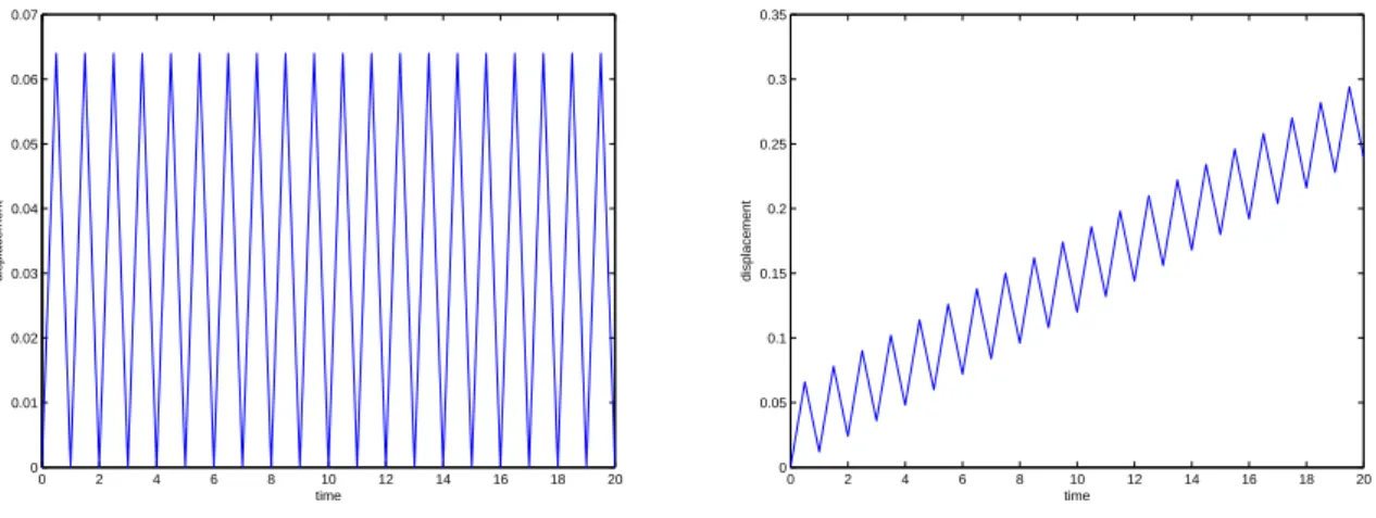
We apply on a rectangular specimen two kind of uniaxial ciclic displacements on its opposite borders, one with constant mean value and the other with a mean value that increases linearly with the time, both illustrated in Fig. 1.
0 2 4 6 8 10 12 14 16 18 20 0 0.01 0.02 0.03 0.04 0.05 0.06 0.07 time displacement 0 2 4 6 8 10 12 14 16 18 20 0 0.05 0.1 0.15 0.2 0.25 0.3 0.35 time displacement
Fig. 1: Applied ciclic displacements: (left) constant mean value; (right) displacement mean value increasing in time
Fig. 2 depicts the stress σxx evolution in both cases (constant and increasing displacement mean
value) at the center of the specimen, both solutions computed without any model order reduction, that is, by applying a standard incremental explicit elastoplastic integration.
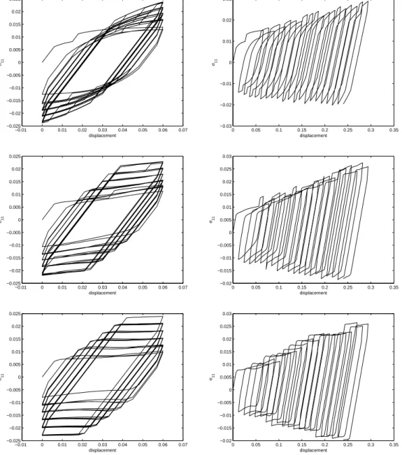
Fig. 4 compares the first three more significant space modes involved in the separated representa-tion of the displacement increment field, that is Xi, i = 1, 2, 3, for both the constant and the increasing
ciclic loadings. Finally from the reconstructed solution at the central point after each solution enrich-ment, Fig. 4 depicts the whole history of the stress versus the applied displacement. It can be noticed that the reduced solutions converge in both loading cases to the reference ones (the ones depicted in Fig. 2) after only 3 enrichment steps.
−0.01 0 0.01 0.02 0.03 0.04 0.05 0.06 0.07 −0.025 −0.02 −0.015 −0.01 −0.005 0 0.005 0.01 0.015 0.02 0.025 displacement σ11 0 0.05 0.1 0.15 0.2 0.25 0.3 0.35 −0.025 −0.02 −0.015 −0.01 −0.005 0 0.005 0.01 0.015 0.02 0.025 displacement σ11
Fig. 2: Stress versus applied displacement at the center of the specimens for both (left) constant and (right) increasing mean value of the applied displacement.
−1 −0.5 0 0.5 1 −1 −0.5 0 0.5 1 function of space 0.1 0.2 0.3 0.4 0.5 0.6 0.7 0.8 0.9 1 −1 −0.5 0 0.5 1 −1 −0.5 0 0.5 1 function of space 0.1 0.2 0.3 0.4 0.5 0.6 0.7 0.8 0.9 1 −1 −0.5 0 0.5 1 −1 −0.5 0 0.5 1 function of space 0.01 0.02 0.03 0.04 0.05 0.06 0.07 0.08 −1 −0.5 0 0.5 1 −1 −0.5 0 0.5 1 function of space 0.01 0.02 0.03 0.04 0.05 0.06 0.07 0.08 −1 −0.5 0 0.5 1 −1 −0.5 0 0.5 1 function of space 0.01 0.02 0.03 0.04 0.05 0.06 −1 −0.5 0 0.5 1 −1 −0.5 0 0.5 1 function of space 0.01 0.02 0.03 0.04 0.05 0.06
Fig. 3: First three space modes involved in the separated representation of the displacement increment
−0.01 0 0.01 0.02 0.03 0.04 0.05 0.06 0.07 −0.025 −0.02 −0.015 −0.01 −0.005 0 0.005 0.01 0.015 0.02 0.025 displacement σ11 0 0.05 0.1 0.15 0.2 0.25 0.3 0.35 −0.03 −0.02 −0.01 0 0.01 0.02 0.03 displacement σ11 −0.01 0 0.01 0.02 0.03 0.04 0.05 0.06 0.07 −0.025 −0.02 −0.015 −0.01 −0.005 0 0.005 0.01 0.015 0.02 0.025 displacement σ11 0 0.05 0.1 0.15 0.2 0.25 0.3 0.35 −0.02 −0.015 −0.01 −0.005 0 0.005 0.01 0.015 0.02 0.025 0.03 displacement σ11 −0.01 0 0.01 0.02 0.03 0.04 0.05 0.06 0.07 −0.025 −0.02 −0.015 −0.01 −0.005 0 0.005 0.01 0.015 0.02 0.025 displacement σ11 0 0.05 0.1 0.15 0.2 0.25 0.3 0.35 −0.02 −0.015 −0.01 −0.005 0 0.005 0.01 0.015 0.02 0.025 0.03 displacement σ11
Fig. 4: Stress versus applied displacement at the center of the specimen for one, two and three terms involved in the separated representation (from top to down) and (left) constant and (right) increasing mean displacement
References
[1] A. Ammar, B. Mokdad, F. Chinesta, R. Keunings. A new family of solvers for some classes of multidimensional partial differential equations encountered in kinetic theory modeling of com-plex fluids. Part II: Transient simulation using space-time separated representation. Journal of Non-Newtonian Fluid Mechanics, 144, 98-121, 2007.
[2] A. Ammar, M. Normandin, F. Daim, D. Gonzalez, E. Cueto, F. Chinesta. Non-incremental strate-gies based on separated representations: Applications in computational rheology. Communica-tions in Mathematical Sciences, 8/3, 671-695, 2010.
[3] A. Ammar, F. Chinesta, E. Cueto, M. Doblare. Proper Generalized Decomposition of time-multiscale models. International Journal for Numerical Methods in Engineering, 90/5, 569-596, 2012.
[4] F. Chinesta, A. Ammar, E. Cueto. Recent advances and new challenges in the use of the Proper Generalized Decomposition for solving multidimensional models. Archives of Computational Methods in Engineering, 17/4, 327-350, 2010.
[5] F. Chinesta, A. Ammar, A. Leygue, R. Keunings. An overview of the Proper Generalized De-composition with applications in computational rheology. Journal of Non Newtonian Fluid Me-chanics, 166, 578-592, 2011.
[6] F. Chinesta, P. Ladeveze, E. Cueto. A short review in model order reduction based on Proper Generalized Decomposition. Archives of Computational Methods in Engineering, 18, 395-404, 2011.
[7] F. Chinesta, A. Leygue, F. Bordeu, J.V. Aguado, E. Cueto, D. Gonzalez, I. Alfaro, A. Ammar, A. Huerta. Parametric PGD based computational vademecum for efficient design, optimization and control. Archives of Computational Methods in Engineering, 20/1, 31-59, 2013.
[8] P. Ladevèze, The large time increment method for the analyze of structures with nonlinear con-stitutive relation described by internal variables, Comptes Rendus Académie des Sciences Paris, 309, 1095-1099, 1989.
[9] D. Ryckelynck, F. Chinesta, E. Cueto, A. Ammar. On the a priori model reduction: Overview and recent developments. Archives of Computational Methods in Engineering, State of the Art Reviews, 13/1, 91-128, 2006.