Estimateurs de calage pour les quantiles

Université de Montréal

Estimateurs de Calage pour les Quantiles

par

Torsten Harms

Département de mathématiques et de statistique Faculté des arts et des sciences

Mémoire présenté à la Faculté des études supérieures en vue de l’obtention du grade de

Maître ès sciences (M.Sc.)

en statistique

aofit

2004

<

l

Université

titi

de Montréal

Direction des bibliothèques

AVIS

L’auteur a autorisé l’Université de Montréal à reproduire et diffuser, en totalité ou en partie, par quelque moyen que ce soit et sur quelque support que ce soit, et exclusivement à des fins non lucratives d’enseignement et de

recherche, des copies de ce mémoire ou de cette thèse.

L’auteur et les coauteurs le cas échéant conservent la propriété du droit

d’auteur et des droits moraux qui protègent ce document. Ni la thèse ou le mémoire, ni des extraits substantiels de ce document, ne doivent être

imprimés ou autrement reproduits sans l’autorisation de l’auteur.

Afin de se conformer à la Loi canadienne sur la protection des renseignements personnels, quelques formulaires secondaires, coordonnées

ou signatures intégrées au texte ont pu être enlevés de ce document. Bien

que cela ait pu affecter la pagination, il n’y a aucun contenu manquant.

NOTICE

The author of this thesis or dissertation has granted a nonexclusive license allowing Université de Montréal to reptoduce and publish the document, in

part or in whole, and in any format, solely for noncommercial educational and research purposes.

Ihe author and co-authors if applicable retain copyright ownership and moral

rights in this document. Neither the whole thesis or dissertation, nor

substantial extracts from it, may be printed or otherwise reproduced without the author’s permission.

In compliance with the Canadian Privacy Act some supporting forms, contact

information or signatures may have been removed from the document. While this may affect the document page count, it does not represent any toss of

Université de Montréal

Faculté des études supérieures

Ce mémoire intitulé

Estimateurs de Calage pour les Quantiles

présenté par

Torsten Harms

a été évalué par un jury composé des personnes suivantes

Christian Léger

(président-rapporteur)

Pierre Duchesne

(directeur de recherche)

Martin Bilodeau

(membre du jury)

Mémoire accepté le:

]o—-1H

SOMMAIRE

Dans la théorie des sondages, les estimateurs de calage, dont l’estimateur

par régression généralisé (GREC) est un cas particulier, représentent souvent la

méthode par excellence pour intégrer l’information auxiliaire dans les estimateurs.

Malgré le succès de cet estimateur, il n’existe pas un estimateur similaire pour

les quantiles ou encore la fonction de répartition. Dans ce mémoire de maîtrise,

un objectif est de développer un estirnateur pour les quantiles qui s’inspire du

concept qui mène à l’estimateur de calage original pour les totaux. Un avantage

de ce nouvel est.imateur par rapport aux alternatives modélistes est qu’il suffit de

connaître les quantiles correspondants pour la variable auxiliaire pour le mettre

en oeuvre, alors que pour les estirnateurs modélistes existants, toutes les valeurs

de la variable auxiliaire doivent être connues, et ce pour chaque unité dans la

population.

On montre que sous certaines conditions, on peut obtenir une représentation

analytique de l’estimateur. De plus, des estimateurs de la variance et des inter

valles de confiance peuvent être élaborés. Comme ce nouvel estimateur est basé

sur le même concept que l’estimateur de calage usuel pour les totaux, on va ana

lyser les parallèles entre les deux et discuter son applicabilité, surtout dans le

contexte des statistiques officielles.

Pour comparer notre proposition avec d’autres estimateurs existants qui uti

lisent aussi de l’information auxiliaire, on va présenter plusieurs études de simula

tion, basées sur des données réelles. Nous constaterons que notre alternative offre

une bonne performance et surtout se montre robuste à une mauvaise spécifica

tion du modèle, dans diverses situations où la population ne suit pas un modèle

iv

linéaire. Cependant, ceci n’est pas le cas pour d’autres estimateurs connus, modé

listes ou non, dont la performance est souvent sensible à la structure des données.

mots clés

estimateur de calage, quantiles, estimateur par le ratio, estimateur

par la différence.

V

SUMMARY

In survey sampling, calibration estimators are often the rnethod of choice in

order to incorporate auxiliary information in the estimation process. A special

case is the generalized regression estimator (GREG). Despite the success of this

estimator, its application is usually limited to the estimation of means or totals of

the population. Particularly, there are no calibration estirnators for quantiles or

distribution functions. The aim of this thesis is to develop a similar estirnator for

quantiles which follows the same concept. as the original calibration estimator for

totals. An advantage of this estimator is that it suffices to know the corresponding

quantile of an auxiÏiary variable, whereas the rnodel-based proposais require the

knowledge of ail values of the auxiliary variable.

We show that, under certain conditions,

we

eau obtain an analytical repue

sentation of this estimator. Variance estimators and construction of confidence

intervals are discussed. Since the new estimator is related to the usual calibration

estimator for totals,

we

_{analyze the similarities between those two and discuss}

possible applications in the area of officiai statistics.

Several simulation studies are presented, in order to compare ouï proposed

estimator with other existing estimators for quantiles which also use auxiliary

information. When the population is not adequately described by a linear modei,

these studies, based on real data, show a robust performance to model misspecifi

cation of

our

proposed estimator. By comparison, other estimators, model-based

or not, are often sensitive to the structure of the data.

Key words

_{Calibration estimators, Quantiles, Ratio estimators, Difference es}

vi

REMERCIEMENTS

Je voudrais remercier Pierre Duchesne et Carl-Erik Srndal pour leur avis

judicieux et leur participation dans ce projet.

Je tiens

aussi

à remercier Ray Chambers pour les commentaires positifs concer

nant l’application des idées développées dans cette recherche.

De pius, je remercie tout le département de statistique de l’Université de

Montréal qui m’a permis de réaliser cette maîtrise. Finalement, merci à mes amis

et ma copine pour leur support.

vii

TABLE DES MATIÈRES

Sommaire

iii

Summary

y

Remerciements

vi

Liste des figures

ix

Liste des tableaux

x

Chapitre 1.

Introduction

1

1.1.

Estimateurs basés sur le plan d’échantillonnage

1

1.2.

Utilisation de l’information auxiliaire

2

1.3.

Estiinateurs de calage

3

1.4.

Recherche existante

4

1.5.

Objectif

5

Chapitre 2.

Théorie des sondages

6

2.1.

Concepts fondamentaux

6

2.2.

Plan d’échantillonnage

Z

2.3.

Estimateur de Horvitz-Thompson

8

Chapitre 3.

Article

10

2.1.

Introduction

11

viii

2.3.

New Calibration Estirnators

16

2.4.

Simulation Resuits

24

2.5.

Concluding Remarks

33

Chapitre 4.

Discussion

43

Annexe A.

Complément d’information pour l’estimation de la

variance

A-i

Annexe B.

Estimateur de la fonction de répartition utilisant la

méthode par le noyau

B-i

Annexe C.

Simulations complémentaires

C-i

ix

LISTE DES FIGURES

1

The population 1V1U284, where y

=

P85 and x

=

P75

40

2

Histogram of the variable P85 in the MU284 population

40

3

The population MU284, where y

=

RMT85 and x

=

REV84

41

4

Histogram of the variable RMT85 in the MU284 population

41

5

The SL1D982 population, where the dependent variable is the taxable

income arid independent variable is the duration of current employment

(in months)

42

6

Histogram of the taxable income in the SL1D982 population

42

X

LISTE DES TABLEAUX

1

Factor

P2k

by age and sex of individual k in the SL1D982 population.

27

2

Comparison of the proposed calibration estimators and of some leading

estimators for quantiles

30

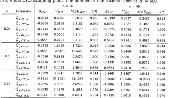
3

Monte Carlo simulation results for sampling from the MU284 population,

y

=

P85, ‘r

P75, under SR$ sampling plan

37

4

Monte Carlo simulation results for sarnpling from the MU284 population,

y

P85,

‘r

P75, under P0 sampling plan

37

5

Monte Carlo simulation resuits for sampling from the MU284 population,

y

RMT85,

‘r =

REV$4, under SRS sampling plan

3$

6

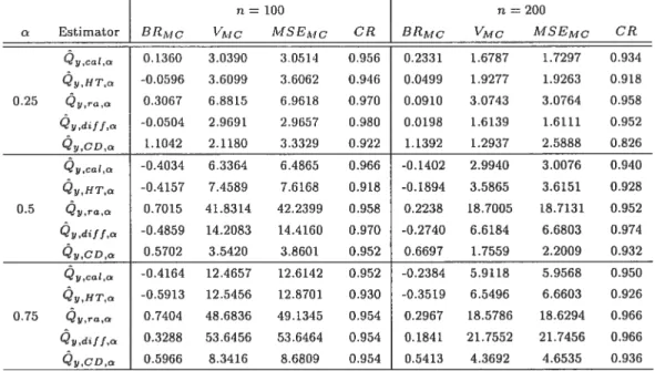
Monte Carlo simulation results for sampling from the $L1D982 population,

under $RS sampling plan

38

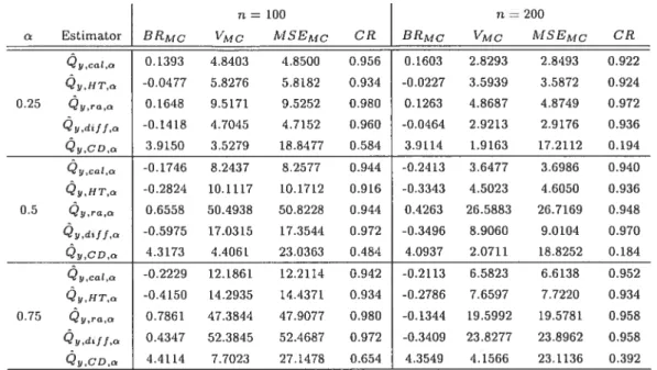
7

Monte Carlo simulation resuits for sampling from the $LID9$2 population,

under P0 sampling plan and the first rule for the construction of the

39

8

Monte Carlo simulation results for sampling from the SL1D982 population,

under P0 sampling plan and the second rule for the construction of

thelrk

39

9

Description des estimateurs par la méthode par le noyau. Tous les

estimateurs utilisent le noyau Gaussien

B-iv

10

Résultats des simulations pour la population MU284, y

=

P85,

‘r =

P75, selon le plan SI avec 500 simulations (à comparer avec Tableau 3

xi

11

Résultats des simulations pour la population MU2$4, y

RMT$5,

x

=

REV$4, selon le plan SI avec 500 simulations (à comparer avec

Tableau 5 dans l’article)

B-v

12

Résultats des simulations pour la population MU281, y

P85, x

=

P75, selon le plan SI avec 500 simulations (à comparer avec Tableau 3

dans l’article)

C-ii

13

Résultats des simulations pour la population MU281, y

=

P85, x

=

P75, selon le plan P0 avec 500 simulations (à comparer avec Tableau

4 dans l’article)

C-iii

14

Résultats des simulations pour la population MU284, y

P85, z

=

S82, sous un plan SI,

n

25 et n

=

50

C-vi

15

Résultats des simulations pour la population MU284, y

P85, x

=

S82, selon le plan P0, n

=

25 et

n =

50

C-vii

16

Résultats des simulations pour la population MU284, y

P85, x

=

S82, sous un plan SI, n

100

C-viii

17

Résultats des simulations pour la population MU284, y

=

P85, x

Chapitre

1

INTRODUCTION

1.1. EsTIMATEuR5 BASlS SUR LE PLAN D’ÉCHANTILLONNAGE

Les estimateurs basés sur le plan d’échantillonnage ont une longue tradition

dans la théorie des sondages. Depuis les travaux pionniers de Neyrnan (1934)

et Hansen et I-lurwitz (1943), ils

ont

offert une façon facile de construire des

estimateurs

pour

des populations finies.

La formulation de ces estirnateurs est assez simple, puisque chaque élément

k dans l’échantillon est habituellement pondéré avec un poids

dk

qui correspond

à l’inverse de sa probabilité de sélection selon le plan d’échantillonnage. Un esti

mateur pour le total, appelé couramment l’estimateur Horvitz-Thompson (selon

Horvitz et Thompson (1952)), d’une variable y se calcule donc comme la somme

des

Yk

dans l’échantillon, chacun pondéré avec le dk correspondant. L’interpré

tation

qu’un

élément k dans l’échantillon doit représenter dk éléments dans la

population semble une explication intuitive naturelle, du fait qu’on sélectionne

un échantillon avec pour objectif de faire une projection sur une population.

En plus de sa construction simple, cet estimateur possède d’autres propriétés

souhaitables. Si chaque élément dans la population a une probabilité non-nulle

d’être sélectionné, on peut montrer que cet estimateur est sans biais dans le sens

que l’espérance sur tous les échantillons possibles est égale au total de la variable y

pour cette population (Sârndal, Swensson et Wretman (1992)). De la même façon,

si les probabilités d’inclusion du second ordre sont toutes non-nulles, il existe des

2

formules simples pour estimer la variance de cet estimateur, et les estimateurs de

variance sont également sans biais.

Contrairement aux estirnateurs modélistes, cet estimateur n’exige aucune sup

position sur la distribution de la variable y dans la population et donc donne des

mesures d’inférence sur la vraie population et non pas sur une population hypo

thétique et infinie qui se comporte selon un modèle spécifié. En contrepartie, cette

propriété peut quelquefois aussi être un désavantage

comme les estimateurs ba

sés sur le plan d’échantillonnage ne suivent pas forcément un critère d’optimalité,

ils sont parfois inférieurs à un estimateur modéliste qui utilise le vrai modèle de

la population.

Néanmoins, à cause de leur simplicité, de leur interprétation naturelle et du

fait qu’ils donnent des mesures d’inférence sur la population finie que le méthodo

logiste désire étudier, ces estimateurs représentent souvent la méthode privilégiée

dans le contexte des statistiques officielles.

1.2. UTILIsATIoN DE L’INFORMATION AUXILIAIRE

Utiliser de l’information auxiliaire sur la population est un concept fort im

portant pour améliorer la performance d’un estimateur. Il est à noter que ceci

est aussi vrai pour les estimateurs modélistes qui exploitent la connaissance d’un

modèle pour la population comme information auxiliaire. Il semble intuitivement

raisonnable que plus on dispose d’information, plus la solution proposée risque

d’être performante et efficace. Normalement, plus on en connaît sur le problème

d’estimation à traiter, plus la solution proposée sera précise et performante. Les

estimateurs basés sur le plan d’échantillonnage ne font pas d’exception à cette

règle.

D’une certaine façon, les estimateurs selon le plan d’échantillonnage ont l’avan

tage qu’ils incluent un type d’information auxiliaire par défaut. En effet, comme

les poids d’échantillonnage sont une fonction des probabilités d’inclusion, une

grande partie de l’information sur le plan d’échantillonnage est déjà intégrée dans

l’estimation. Ainsi, dans l’évolution des estimateurs discutés jusqu’à maintenant,

les plans stratifiés développés par Neyman (1934) illustrent très bien ce propos.

3

En effet, en général ces plans sont à probabilités inégales et ils permettent d’avoir

des poids d’échantillonnage différents selon des mesures de taille.

Il existe néanmoins un autre type d’information auxiliaire: la connaissance de

variables auxiliaires qui sont corrélées

avec

la variable d’intérêt. Il arrive fréquem

ment qu’on connaît par exemple des variables socio-déinographiques sur tonte la

population cible. Cette information additionnelle peut être utilisée pour améliorer

la précision de l’estimation.

1.3. EsTIMATEuRs DE CALAGE

Dans le cas des estimateurs basés sur le plan d’échantillonnage et surtout pour

l’estimateur Horvitz-Thompson, la méthode la plus fréquemment appliquée pour

incorporer de l’information auxiliaire est la technique des estimateurs de calage.

Ce concept a été développé par Deville (1988) et s’est popularisé rapidement.

Le concept fondamental de cet estimateur est de remplacer les poids dk dans

l’estimateur de Horvitz-Thompson par des poids modifiés

Wk

qui doivent être les

plus près possible des poids originaux, mais en satisfaisant des contraintes qui

impliquent l’information auxiliaire. Plus précisément, on exige que l’estimateur

correspondant, appliqué aux variables auxiliaires, doit reproduire correctement

les totaux connus pour ces variables dans la population.

En plus de son interprétation facile avec les poids modifiés, cet estimateur est

aussi relativement facile à appliquer. Si on mesure la proximité entre les vecteurs

de poids w

(wk)kES

et d

= (dk)kES

par la distance euclidienne, il est même pos

sible d’obtenir des formules analytiques pour les poids

Wk.

De plus, pour ce nouvel

estimateur, on peut étudier facilement les concepts fondamentaux des estimateurs

basés sur le plan d’échantillonnage. Par exemple, il existe des formules similaires

pour la variance, l’estimation de la variance et les intervalles de confiance (voir

Deville et Sirndal (1992)).

Un domaine de prédilection pour le calage est la statistique officielle. Nor

malement, des échantillons de grande taille sont disponibles qui rendent d’autres

estimateurs modélistes trop coûteux. Dans un contexte de statistique officielle, il

est naturel de connaître de l’information auxiliaire sur la population, en raison

4

d’un recensement passé ou d’autres enquêtes de grandes envergures, en cours ou

répétitives.

Un autre avantage du calage, qui n’est pas toujours explicitement mentionné,

est le fait qu’il peut être utilisé afin d’homogénéiser différentes enquêtes. Ceci veut

dire que différentes enquêtes sur la même population cible donnent les mêmes

(et même exacts) estimateurs pour certaines mesures clés, comme la taille de

la population ou certains totaux particulièrement importants (par exemple les

variables âge et sexe).

Tenant compte de toutes ces réalités, il n’est pas surprenant que les techniques

de calage soient souvent adoptées par les agences statistiques gouvernementales

d’importance. Par exemple, pour Statistique Canada, cet estimateur est l’outil

principal pour incorporer de l’information auxiliaire, et le logiciel correspondant,

appelé le Système Généralisé d’Estimation (ou en anglais GES, pour Generatized

Estimation System) est aussi commercialisé dans plusieurs pays (voir Estevao,

Hidiroglou et $iirndal (1995)).

1.4. RECHERCHE EXISTANTE

Jusqu’à maintenant, la recherche a comporté en deux grandes parties. Premiè

rement, dans les fondements plus théoriques du calage. Voir par exemple Sârndal

et Deville (1992), qui ont montré qu’il existe un lien entre l’estimateur de calage

et l’estimateur par régression généralisé. En fait, si la taille de la population tend

vers l’infini, ces deux estimateurs sont convergents et asymptotiquement équiva

lents. De plus, ils ont montré que, pour les populations de grande taille, le choix

des différentes fonctions de distance entre w et d n’est pas trop important.

D’un autre côté, une multitude de modifications pratiques pour ce type d’es

timateur ont été développées. Un exemple est le travail de Estevao et Sârndal

(2002), qui préconise une méthode de calage en deux phases

une première étape

de calage au niveau de l’échantillon pour traiter la non-réponse et subséquemment

l’application de l’estimateur de calage au niveau de la population pour corriger

des erreurs échantillonnalles.

1.5. OBJEcTIF

Avec tous ces travaux et la popularité de l’estimateur de calage, il n’en demeure

pas moins que la recherche existante se concentre principalement sur l’estimation

des moyennes ou des totaux. Si on adopte le concept sous-jacent au calage, il

pourrait être tentant de l’appliquer à d’autres paramètres d’intérêt. Après une

introduction à la théorie des sondages, un article, dont un des auteurs est l’auteur

de ce mémoire, explore cette idée en utilisant le concept d’estimateur de calage

pour les totaux, pour développer cependant un estimateur pour les quantiles.

L’objectif n’est pas seulement de déduire un estimateur similaire pour les quantiles

ou fonctions de répartition. En plus, on veut établir des parallèles entre ces deux

estimateurs, afin d’analyser ses propriétés analytiques ainsi que son application

en pratique par des simulations réalistes dans des populations réelles.

Chapitre

2

TH1ORIE DES SONDAGES

Le but de ce chapitre est d’introduire les concepts de base de la théorie des

sondages pour un lecteur qui n’a pas une connaissance approfondie dans ce do

maine. Tous les points développés ici se trouvent également dans l’ouvrage de

Sirndal, $wensson et Wretman (1992).

2± CONCEPTS FONDAMENTAUX

Une particularité fondamentale dans la théorie de l’échantillonnage est le fait

qu’on travaille avec une population finie, dénotée par U

{1,.

.

,k,.

. .

,N}.

Ceci est différent de l’approche standard en statistique qui présume souvent une

population infinie. Avec chaque étiquette k, les valeurs de plusieurs variables

peuvent être associées. Pour une variable d’intérêt y, la valeur de cette variable

pour l’élément k est dénotée

_Yk

On note que ces valeurs sont considérées fixées.

Dans la population U, un échantillon

s

est selectionné à partir duquel on veut faire

des conclusions sur la population totale et inconnue. On note que l’échantillon

s

est sélectionné d’une façon aléatoire parmi l’ensemble de tous les échantillons

possibles S, mais le mécanisme qui détermine cet échantillon doit être déterminé

et connu, pour porter des conclusions valides sur la population.

Le but est souvent d’estimer le total d’une variable y dans la population. On

note ce total T

₌ Yk

(la notation

A’

A

C

U va être utilisée partout dans ce

mémoire pour

_kEA)

De manière plus générale, on veut effectuer des décisions

inférentielles valides basées sur l’échantillon

s.

z

2.2.

PLAN D’ÉCHANTILLONNAGE

Comme mentionné plus haut, l’échantillon

s

est déterminé selon un mécanisme

aléatoire, mais il doit être connu. Dans la théorie des sondages, ce mécanisme est

le plan d’échantillonnage et il est un des objets centraux dans la théorie des

sondages. Seulement avec un plan d’échantillonnage complètement connu, nous

sommes en mesure de faire de l’inférence valide sur les estimateurs dérivés. Le

plan donne la probabilité de sélection

p(s)

pour chaque échantillon

s

e

S.

Une quantité importante induite par le plan d’échantillonnage est la

pro

babilité d’inclusion dans l’échantillon. Soit I(k

E s)

la fonction indicatrice qui

est 1 si k

E s,

et zéro sinon. Alors la probabilité d’inclusion pour un élément

k

e

U est donnée

par

lCk

= ZSEsI(k

e

s)p(s).

De la même manière, la proba

bilité d’inclusion du second ordre pour deux éléments k, t

_e

U est donnée par

k1

_{ZsES I(k}

E

s)I(t é

s)p(s).

On note immédiatement que

7Ukk

=

Dans l’article qui suit, nous allons souvent faire référence à deux plans d’échan

tillonnage particuliers : le plan aléatoire simple, dénoté par SI et le plan de Pois

son, que l’on note P0. Pour le plan SI, on fixe d’abord la taille de l’échantillon

n

<

_{N. Ensuite tous les échantillons}

_s

_{U qui sont de taille n se voient attribuer}

la même probabilité de sélection

()1.

Par conséquent, on peut montrer que

n/N pour tout k

E

U et

rrkt

=

pour tout k, t

E

U avec k

t.

Comme

on peut le voir, ce plan correspond à une sélection aléatoire simple sans remise de

n parmi N éléments de U. L’autre plan, qui

va

être utilisé dans ce mémoire est

le plan P0. Pour ce plan, chaque élément k

E

U est assigné

une probabilité de

sélection

7k >

O, et les probabilités d’inclusion ne sont pas forcément les mêmes.

Après, chaque élément k est sélectionné avec probabilité 7rk indépendamment des

éléments déjà sélectionnés. Comme chaque élément peut entrer dans l’échantillon

s

ou pas, il y a

2N

différents échantillons possibles. Une autre conséquence est

que la taille échantillonnalle n’est pas fixée. On note aussi que les probabilités

d’inclusion de second ordre pour k

t sont simplement

“kt

=

Il existe d’autres plans beaucoup plus sophistiqués qui peuvent se composer

de plusieurs phases ou utiliser de l’information sur la partie de l’échantillon déjà

8

observée. Une description de plusieurs de ces plans et leur utilité dans certaines

situations ont aussi été traités par Sirndal, Swensson et Wretman (1992).

2.3. EsTIMATEuR DE

HORVITZ-THOMPSON

Un estimateur relativement simple qui sert aussi comme référence pour la

plupart des autres estimateurs est l’estimateur de Horvitz et Thompson (1952).

Comme mentionné dans l’introduction, cet estimateur est basé sur le concept na

turel, que chaque élément dans l’échantillon représente un certain nombre d’élé

ments dans la population totale. Dans le cas de l’estimateur de Horvitz-Thompson

(HT), on donne à chaque élément k

e s

un poids

dk 7T’.

Comme on va le voir,

ce choix des dk implique des propriétés désirables pour cet estimateur. Néanmoins,

il peut arriver que pour des éléments avec une probabilité de sélection très petite,

les poids correspondants donnent trop d’influence à ces unités. Basu (1971) a ex

ploré ce problème et mentionné que ce n’est pas principalement un problème de

la méthode de pondération, mais bien un problème de stratégie mal conçue (la

stratégie étant ici l’utilisation d’un estimateur Horvitz-Thompson avec un plan

d’échantillonnage mal adapté).

Dans le cas de l’estimation du total d’une variable y, l’estimateur Horvitz

Thompson est alors la somme des

Yk

dans l’échantillon

s,

chacun pondéré avec le

poids

dk

=

Pour analyser les propriétés de cet estimateur, on dénote par E(.) l’espérance

sous les différents échantillons possibles. Plus précisément pour un estimateur

m(s)

qui dépend de l’échantillon sélectionné, on définit E(m)

= sm(s)p(s).

Pour l’estimateur Horvitz-Thompson on peut montrer (voir par exemple Siirndal,

$wensson et Wretman (1992)) que E(Î’,HT)

=

T, impliquant que l’estimateur

est sans biais selon le plan d’échantillollnage.

Si on définit la variance échantillonnalle par V(m)

=

E[{m—E(m)}2], $àrndal,

Swensson et Wretman (1992) ont aussi constaté que

- YkYt

V(T,HT) =

9

où

Akj = kt — k’rt.

Cette variance peut être estimée par

k1YkYt

—,

k1 7rk 7r1

ce qui forme une expression utile dans la construction des intervalles de confiance.

De plus, on a

E((i,,HT)) =

V(f,ffT), impliquant que la variance est aussi

estimée saris biais.

L’article présenté dans le chapitre suivant va traiter d’une modification de l’es

timateur de Horvitz-Thompson. Il est question d’estimateurs de calage, comme

ceux qui sont présentés dans l’introduction. Ces estimateurs permettent d’utiliser

de l’information sur des variables auxiliaires pour améliorer la performance de

l’estimation; par exemple, dans un esprit de réduction de la variance et d’effica

cité.

Chapitre

3

ARTICLE

Le présent chapitre consiste en une copie intégrale de l’article ‘On Calibration

Estimators for Quantiles’, tel que soumis au journal

$urvey Methodotogy

en juin

2004 et révisé en novembre 2004. Le premier auteur de l’article est aussi l’auteur

du présent mémoire.

On Calibration Estimation for Quantiles’

December 1, 2004.

Torsten HARMS

Université de Mon tréal

a nd

Pierre DUCHESNE

Université de Mon tréal

ABSTRACT

In this paper, we _{consider the estimation of quantiles using the calibration paradigm. The}

proposed methodology relies on an approach similar to the one leading to the original calibra tion estimators of Deville and Srndal (1992). An appealing property of the new methodology is that it is not necessary to know the values of the auxiliary variables for ah units in the population. It suffices instead to know the corresponding quantiles for the auxiliary variables. When the quadratic metric is adopted, an analytic representation of the cahibration weights is obtained. In this situation, the weights are similar to those leading to the generalized re gression (GREC) estimator. Variance estimation and construction of confidence intervals are discussed. In a small simulation study, a calibration estimator is compared to other popular estimators for quantiles that also make use of auxiliary information.

Key words and phrases: Calibration estimators; Quantiles; Ratio estimators; Difference esti mators.

1. INTRODUCTION

In recent years, considerable attention has been given to the estimation of population distribution functions in the context of survey samphing. A particular target of this attention has been the median, which is often regarded as a more satisfactory location measure than the mean, especially when the variable of interest follows a skewed distribution. Traditional

‘Abbreviated title: “On Cahibration Estimation for Quantiles”.

Corresponding author: Pierre Duchesne, Université de Montréal; Département de mathéma tiques et de statistique; CP 6128 Succursale Centre-Ville; Montréal, Québec H3C 3J7; Canada. tel: (514) 343-7267; fax: (514) 343-5700; e-mail:

12

estirnators of population means or totals cari be usually substantialiy improved if relevant auxiliary information is made available. Consequently, the use of such auxiliary information seerns highly desirabie in sample quantiic estimators.

Using a rnodel-based approach, Chambers and Dunstan (1986) considered quantile es timators based on an estimator of the distribution function which do incorporate auxiliary information. Rao, Kovar and Mantel (1990) have proposed design-based alternatives to the model-based approach. They used simulation experirnents to compare two quantile estimators, based on ratio and difference estimators, to the simple design-based estimator which makes no use of the auxiliary information. It should be noted that neither of the two design-based proposais requires knowledge of the auxiliary information for each unit in the population; it rather suffices to know only the corresponding quantiies. While the model-based estimator proposed by Chambers and Dunstan (1986) can 5e more efficient than its design-based alter native if the model is correctly specified, Rao et aÏ. (1990) have pointed out the advantage of the design-based estimators under model misspecification. Chambers, Dorfman and Hall (1992) have compared these two estimators theoretically with respect to their consistency, asymptotic bias and variance under a population model. Their main conclusion is that neither of the two methods is a sharp winner. Dorfman (1993) has reevaluated the simulation resuits obtained by Rao et aÏ. (1990) and proposed a modified version of their methodology, using model-based arguments. Variance estimators in the model-based approach of Chambers and Dunstan (1986) and the design-based estimators of Rao et aÏ. (1990) are discussed in Wu and Sitter (2001).

Other related works on quantile and median estimators include that of Kuk (1988) who proposes quantile estimators under pps (proportionat to size) sampling and that of Kuk and Mak (1989) who use a method that is based on cross-classifying the individuals in the sample, according to the variable of interest and a single auxiliary variable. Meeden (1995) takes a diffèrent approach to construct a median estimator based on univariate auxiliary information, using the Bayesian concept of Polya sampling to impute ail the target variable’s unknown population values via a ratio-based approach. Rueda, Arcos and Martfnez (2003) have recently built quantile estimators that extend ratio, difference and regression estimators in ways similar to those developed for the population mean.

In this paper, we follow the concept of calibration which was first introduced by Deviiie (1988) in order to derive a quantile estimator. The calibration approach has gained popularity

13

in real applications, because the resulting estimators are easy to interpret and to motivate, relyirig, as they do, on sampling weights and natural calibration constraints. This approach was developed in the seminal work of Deville and Sàrndal (1992) as an alternative means of incorporating auxiliary information in the estimation of population totals. The so-called calibrated weights are found by minimizing a distance measure between the sampling weights and the new weights, which need to satisfy certain calibration constraints. For estimating totals the calibrated weights replace the original design weights used in Horvitz-Thompson type estimators. When the new weights are applied to the auxiliary variables available in the sample, they reproduce the known population totals of the auxiliary variables exactly; it is for this reason that the estimators in this class are called calibration estimators. See also Singh and Mohi (1996) who provide simple justifications of calibration estimators. They also present a very general and unifying treatment of calibration methods whose weights satisfy certain range restrictions and benchmark constraints.

Our fundamental aim is to propose calibration estimators for quantiles which are as easy to implemerit and interpret as the calibration estimators for totals developed by Deville and Sàrndal (1992). When compared to the quantile estimators available in the literature, the new calibration estimators should also be competitive with respect to their bias, variance, and coverage rates of the confidence intervals. farly calibration estimators for distribution func tions and quantiles include those proposed by IKovaevi (1997), who considered estimators of the distribution function calibrated on moments of the auxiliary variables. Harms (2003) has investigated a similar approach, with applications to the Finnish European Household Panel survey. Ren (2002) appears to have been the first to develop a unifying treatment of calibration estimators for distribution functions and quantiles. The calibration estimators for quantiles presented in this paper continue the work initiated by Ren (2002). We adhere to the original calibration paradigm for totals as closely as possible: when the parameter of interest is a total, it seems natural to calibrate on totals of the auxiliary variables. In the present context, since the parameter of interest corresponds to a quantile, the calibration constraints require that the weights are such that the sample quantile estimators of the auxiliary vari ables and their corresponding population quantiles are equal. In other words, the weighted quantile estimators for the auxiliary variables should yield exactly the population quantiles, which are assumed to be known. We present arguments which justify calibrating on quantiles, whenever the parameter of interest is itself a quantile. Interestingly, our methodology does not

14

necessitate knowledge of the values of the auxiliary variables for ail units in the population. Since the resulting estimators display a structural form very similar to the original calibration estimators for totals, it is expected that, under general conditions, the proposed estimators for quantiles vill be asymptotically design-unbiased. Furthermore, these similarities allow us to derive variance estimators which admit a familiar form. Contrary to some of the other estimators, the proposed approach is also applicable to vectorial auxiliary variables (that is, when several auxiliary variables are available), while requiring only minimal auxiliary infor mation. However, some restrictions may apply when the sample is highly unrepresentative of the sampled population or when the quantiles being estimated are very close to the population minimum or maximum. Note that highly unrepresentative samples cari also cause problems for calibration estimators for totals commonly used; in such situations, the algorithm for com puting calibration estimators may fail to converge for many distance measures of practical interest.

The organization of the paper is as follows: In Section 2, some preliminaries are given, in cluding a brief review of the calibration estimators for totals. The new calibration estimators for quantiles are developed in Section 3.1. The standard distribution function can be inter preted as a Horvitz-Thompson estimator, providing a possible approach to the construction of a calibrated distribution function estimator. Quantile estimators are then naturally derived by inverting the distribution function estimator (see e.g., Ren (2002)). As in calibration esti mators for totals, design weights cari be replaced by more general sampling weights, in order to take account the auxiliary information. However, for many situations of practical interest, it may happen that no solution exists for the calibration constraints when this kind of distri bution function estimator is adopted, the reason being that this estimator corresponds to a step function. In order to avoid existence problems of solutions for the calibration constraints, a new distribution function estimator is introduced, based on the natural concept of inter polation. Under the common quadratic metric, an analytic representation of the calibration weights is provided in Section 3.2; variance estimators and confidence intervals are discussed in Section 3.3. A practical aspect involves evaluating the methodology proposed with real popu lations and several sampling plans. Consequently, in Section 4, we present a small simulation study where we compare our new approach, with respect to variance, bias and coverage rates of the confidence intervals, with that of Chambers and Dunstan (1986) as well as with some of the estimators proposed by Rao et al. (1990). Finally, concluding remarks are offered in Section 5.

15

2. SOME PRELIMINARIES ON CALIBRATION ESTIMATORS

In this section, we present the fundamental concepts and notations useful for the sequel. We also give a brief review of calibration estimators for totals.

Let U {l,... ,k,... ,N} be a finite population of size N. Let T ZUYk be the

population total of the variable of interest y, (note that for a set A, A E U, _{ZA will be used}

as shorthand for _ZkEA). A sample s C U of size n is drawn according to a sampling plan. Let 7rk Pr(s k) and rkt = Pr(s k,t) be the first and second order inclusion probabilities,

respectively. We denote the design weights dk ir’ and Ty,HT

_Z5

dkyk represents the

Horvitz-Thompson (HT) estimator of T.

Let xk = (xlk, .. ,xJk)’ be a vector of auxiliary variables associated with unit k, k

e

U. Calibration estimators naturally include auxiliary information in the estimation. Let

s = {k1,... ,k}, s C U. Starting with the vector of original weights d = (dk1,.. . ,dkj’,

new weights are found which, when applied to the auxiliary variables available in s, make it

possible to retrieve the known population totals for the J auxiliary variables T = =

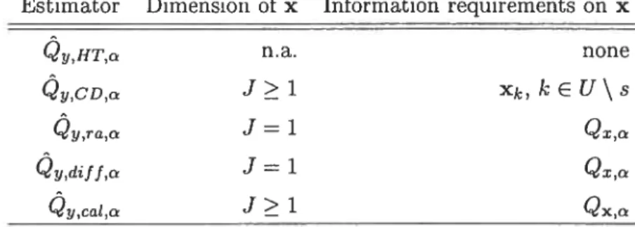
(T1,... ,T )‘. The calibration estimator for totals are more precisely defined in Definition 1. Definition 1 (Calibration estimator for totals). Let d = (dk1,... ,dkj’ be the design

weights. The calibration estimator for totats takes the form Ty,caj =

Zs

WksYk, where the

weights Wks, k E s are obtained as the fottowing minimization probtem with Tespect to the

variabte y = (vk1,. ,vkj’:

w = argrnin D(v, d), (1)

subject to the catibTatron constraints

Zs

VkXk = T, where D(.,.) denotes the distance measure

and w (wki,. . . ,Wkj corTesponds to the vector of the catzbrated weights.

For notational simplicity, we write wk Wk5 in Definition 1 when no confusion is possible.

It is common practice to let xlk 1, Vk

e

U, and consequently T1 = N. This means that

the calibrated weights satisfy the natural constraint

_>

= N. Many distance functions

D are available in the literature (see, e.g., Deville and Siirndal (1992), Chen and Qin (1993), Thompson (1997)). Consider the quadratic distance function

D(v,d) =

(vk—dk)2

(2) where _q determines the importance of the unit k

e

s in the calibration problem. Het

16

the optimization problem (1) using the Lagrange multiplier technique (see Deville and Sàrn

daT (1992), among others), the weights uk = dk(1 + qk4Às) _{are obtained, where À} =

dkqkxx)’(T — Fx,IT) and ‘tx,HT denotes the HT-estimator of T. This choice of distance function leads to the weights of the well-known generalized regression estimator

(GREC) of Cassel, SirndaÏ and Wretman (1976), which is studied in detail in Sàrndal, Swens

son and Wretman (1992). Under minimal requirements for the distance measure D, Deville and Sârndal (1992) have shown that ail calibration estimators in this class are asymptotically equivalent to the GREG. For case of interpretation and other cosmetic reasons, sorne users may want to have positive weights or restrict them to a specific interval (sec also Singh and

IViohi (1996)). In practical applications, these numerical features of the weights seem to be

the main motivation for an alternative choice of D.

3. NEW CALIBRATION ESTIMATORS

In this section we develop calibration estimators for quantiles, using ideas similar to those leading to the calibration estimators for population totals, as described in Section 2. The new

calibration estimators for quantiles are introduced in the next subsection, using interpolated distribution function estimators. Then, special attention is devoted to the quadratic distance

function. The last subsection prescrits variance estimation and the construction of confidence intervals.

3.1 Definition of the calibration estimators for quantiles Let

_Qx,c,

_(Qx,a,.

. . ,

Q,)’

denote the known vector of population quantiles for the

vector of auxiliary variables xk = _{(X 1k,-•} ,xjk)’, k E U. The Heavysicle function H(z) is

given by:

f

1 z>0, z<0.

The population distribution function of a scalar auxiliary variable x is defined in the usual

way as F(t) = N—’ H(t

— Xk), and the population quantile

Q

is obtained by letting

= inf{t F(t) cr}.

The vector

_Qx,a

_{contains quantiles of the auxiliary variables, obtained from information in} past surveys or from available administrative sources. For example, for skewed distributions

17

the record files the population medians rather than population means; in this case it seems natural to assume the knowledge of Qx,o.5. This suggests that, using the same approach as the one leading to calibration for totals described in Section 2, the proposed estimator for the population quantile

_Qy,a

of the variable of interest y, noted could be obtained by inverting a certain estimator of the distribution function (that we discuss below), subject to calibration constrairits such as

j

= 1,. .., J. Following the usual inter

pretation, if the calibrated weights allow us to retrieve the known population quantiles of the auxiliary variables then, under certain conditions, they should produce reasonable estimators for the quantile of the variable of interest y.

More precisely, the calibrated weights are obtained by solving the following optimization problein:

w = argmin D(v,d), (3)

subject to the calibration constraints Vk = N and _x,ca1, ,_{“Zxj,cai,c)’} =

Q

The estimators x,cat,a and

Jy,cat,a

rely on the vector of weights w, stemming from the solution of the calibration problem (3). To calculate these estimators for quantiles, we need to construct w-weighted estimators of the distribution function for variables x and y. Based on the sampling weights d, a natural estimator of the sampling distribution function is given by

= dH(t

— Yk)/ d, (4)

which provides a consistent estimator of F (t). Similarly, (t) can be consistently esti mated by F(t) = ZdkH(t—xjk)/Z8dk,

j

= 1,... ,J. A w-weighted distribution function

estimator of (t) is given by

Èxj,cat(t)

= wH(t

— Xjk)/

>

Wj. (5)

A similar formula holds for

_-y,cat

(t). These w-weighted estimators are considered in Ren (2002). However, if one estimates by = inf{t

I

.‘(t) a}, or makes a similar

estimation using a w-weighted version, then it is generally not possible to reach an exact so lution of the calibration problem (3). Indeed, if the previous definition is used to estimate the quantiles by inverting the distribution function using the previous definitions, then the constraints in the optimization problem (3) will not, in general, be fuffilled unless the sample s contains precisely a unit k such that Xjk =

Q,a.

When J is large, this problem can be more

18

pronounced. Furthermore, even if the sample does contain siich a value, it is sometimes not possible to obtain the weights needed to minimize the distance function, the reason being that under certain circumstances, the weights fuffihling the calibration constraints form an open set, whereas the optimal weights lie precisely on the border of this set. The following example illustrates this situation.

Example 1:

Consider a population U of size N = 30, such that the population median of z is Q1,o = 2.

A sample s of size n = 3 is drawn, and suppose that xk = k, Vk

e

s = {1, 2, 3}. For

simplicity, the distance measure D(v, d) = — dk)2 is adopted; it is supposed that

the sampling weights are (d1,d2,d3) = (15,9,6). Based on (5), the calibration constraint

S Qx,cat,O.5 = inf{t

I

Fx,cat(t) 0.5} = 2, which implies that

Z9

_wkH(2 — xk) > 15 and

wH(l — xk) < 15. Equivalently, w1 + W2 > 15 and w1 < 15. Thus we have to

choose w1 of the form w1 = 15 — e, for e > 0. In this case, since w1 + w + w3 = 30,

we have that D(v,d) E2 + (w2 — 9)2

+ (w2 9 — e)2 leading to the optimal solution

(wi,w2,w3) = (15—e,9+e/2,6+e/2). Consequently, for these weights D(v,d) 3e2/2, which

is obviously minimized when e —+ 0. However, the limit reduces to w = (w1, w2, w3) = (15, 9, 6)

with D(w, d) = 0, but based on these weights _Qx,cai,O.5 1 _Qx,O.5 = 2.

However, these difficulties can be naturally avoided by considering a smooth estimator of the distribution function. For simplicity, we consider here a distribution function estirnator calculated using a linear interpolation (another possibility is discussed in Section 5), which is precisely defined in Definition 2.

Definition 2 (Interpolated distribution function estimators). Define r

Z

wkff,8(t,Yk) Fy,catt) = , 6 wk wkH,8(t,Xjk) F. cai(t) = (7)

Z3

wk

where the Heavyside function H in

₍₎

and (5) is rcptaced by the stightty modified function

1, _Yk

H,5(t,_Yk) = t3,3(t), _Yk = U,3(t), (8)

19

where L,3(t) = max{{yk,k E s <t}U {—oc}}, U,5(t) = min{yk,k E s Yk > t} U {oo}}

and /3,(t) = {t— L,,,8(t)}/{U,5(t) — L,8(t)}. The fnnctiori H,S(t,xk) is defined simitarty.

The estimators (6) and (7), based on the fnnctions _{Yk) and H13,(t, xk), are catted} interpotated distTib’at2on fnctzon estirnators of F(t) and F1 (t), Tespect%vety.

The various quantities in (8) have easy interpretations: L,3 and represent the lower and upper neighbors of t in the sampled values Yk k E s, and ,5(t) denotes the linear in terpolation coefficient between these two quantities. In particular, for ail t E {Yk ,k E s} we

have H,5(t,yk) = H(t

— yk). Consequently, the relations

Êy,cat(t)

= .y,cat(t) are satisfied for

ail t E _{Yk ,k E s}. For ail the other values of t, _Êy,cat(t) consists of a linear interpolation

between these quantities. In the following example, Exampie 1 is revisited using the interpo lated distribution function estimator (Z).

Example 2:

In Example 1, using the interpolated version (Z), the constraints are now w1 + w2 + w3 = 30

and (w1 + w2)/(wl + w2 + w3) 0.5. Consequentiy w3 = 15, w1 + w2 = 15. Simple algebra

shows that the optimal solution is (w1,w2,w3) (10.5,4.5, 15), which is now well-cÏefined.

With the interpolated distribution function estimators, .1(a) and _at(Ù) are now

well defined a-quantile estimators for ail ci E (0, 1), as long as one can assure that the weights

wk are ail strictly positive. Letting _{Ê’cat(ci), we deftne the proposed calibration}

estimator _2y,cat,c for the quantile using the interpolated distribution function estimator given in Definition 2.

Definition 3 (Calibration estimator for quantiles). Consider tue optimization prob

terri (3,), subject to the catibration constraints

_>

vI, = N and_{(x,ca1, (Zx1,cat,c,..}

, L2xj,catc)’

Qx,a. Sotuing this optimization probtem md denoting hie Tesuttzng wcights as w, the proposed

catibratiori estzmator foT quantites of is defined by

2y,cat,ft

=

at(Ù),

(9)

where Êy,cai(t) iS given by (6).

One of the appealing properties of the proposed estimator (9) is that it yields exact popula

20

Assume that _Yk = a + bzk holds perfectly for ail units k é U and suppose that the units in the

sample s are such that xk < < x for sorne units xk and x1, k, t ê s. For the calibrated estimator (9), we have that Pxcai(Qxc) = n. We need to distinguish the two cases, b > O

and b < O (The case b = O is trivial since _Yk is then identically equal to a constant). Firstly,

consider the situation b > 0. Since the linear relation _Yk a+bxk is satisfied for ail units k and

since b >0, the following relations hold: L,5(a+bt) =a+bL,(t); U,(a+bt) a+bU,3(t)

and ,,3(a + bt) = These relations lead to H,5(a + bt,yk) H,5(t,zk). It follows that

_Êy,cai(a

+ bL) Êx,cat(t). Furtherrnore,

Êy,cat(a

+ bQi,a) = a and using the relation

a + we deduce that Êy,cai(Q,a) c. Consequently, when an exact linear rela tionship holds and b> 0, 2y,cat, =

Êjat()

= $econdly, consider the case b < 0. We

deduce in this case the following relations: L,(a+bt) a+bU,8(t); U,5(a+bt)

t3y,8(a + bt) 1 — i3,(t) and Hy,3(a + bt,yk) 1— H,(t,xk). Since b < 0, the relationship

between the quantiles of x and y is given by a + Then, we deduce that

Êy,cat(Qy,_c)

Êy,cat(O

+ bQx,a) 1 —

Êxcat(Qrcj

= 1 — a. Thus, in this situation,

Qy,i—a

is estimated exactly by This meatis that, when an exact relation holds, if b > O the

proposed calibration estimator

_y,cat,c.

yields perfect estimators with zero bias and variance of On the other hand, if b < O and calibrating on

_Qy,1—Q

is estimated exactly by

y,cat,1—

(which makes sense because the perfect linear relationship between x and y is such that the siope parameter is negative).

Note that when

Êy,cat

and

_Êxj,cat

are invertible at points

_Qy,a

and the calibration constraints in (3) can be rewritten in terrns of the distribution functions, that is the calibration constraints based on the quantiles are equivalent to

_{ÊXj,cat(QXj,Q)}

= a,

j

= 1,...

,

J. This

means that the original calibration problem can be alternatively written in terms of distribution functions with the above constraints.

A natural question arises as to the existence of a solution to the optimization problem (3). Even when formulated with the interpolated distribution functions, it is not always possible to find a solution to (3). For example, if is smaller or larger than ail values Xjk in the sample

s, then

Ès cat(Qz )

will equal zero or mie regardless of the choice of the weights w. Thus in these cases it may happen that the calibration constraints cannot be fulfilled. However, when the sample’s behavior differs widely from that of the target population, one should keep a very critical eye on any adjustment, and this situation can be considered somewhat extreme. In practice, this rarely occurs unless is chosen very close to zero or one. Note that it may

21

be impossible to obtain a solution when the sample size n is small. In these situations, the sample minimum or maximum could serve as a possible estimator or we could resort to the simple design-based estimator of the distribution function.

The second potential problem is that sorne weights wk might be negative. In this case

Fy,cat

is no longer bijective. This is not a problem as long as

1at(a)

is stiil uniquely determined. This problem can be avoided by restricting all the weights to be strictly positive, using an appropriate metric D(.,

_.).

This approach has been adopted by Kovaevi (1997) (for more details on distance functions yielding positive weights, sec also Deville and Sàrndal (1992) and Singh and Mohl (1996)).

Remark 1:

The proposed distribution functions estimators (6) and (7) rely on a linear interpolation. In a unified way, the population distribution function, which is a step function as well, could also be defined using a linear interpolation. In practice, the two definitions differ only slightly in behavior, if the population N is sufficiently large. However, it should be noted that if the population size N is relatively small, it might be worth using an interpolation to define distribution functions.

Remark 2:

In the optimization problem (3), we calibrated on a particular quantile. This approach could be extended by allowing to calibrateon a finite set of quantiles, if such information is available. More precisely, suppose that for an auxiliary variable x, the mqUantileS in 1,... ,M are known, where M < n — 1. In this case, we could consider the calibration constraints

Êx,cai(Qx,c,j

= in = 1,... ,M and solve the optimization problem (3) with these addi tional calibration constraints. Naturally, this information yields a more complete description of the distribution of the auxiliary variables; so the efficiency of the calibration estimators is expected to be higher.

Remark 3:

The proposed calibration estimator (9) is obtained by calibrating on population quantiles. An other possibilityhas been considered by Ren (2002) who calibrated on population moments, up to order m, of the same distribution. More precisely, Ren (2002) has proposed calibration

es-22

timators for quantiles satisfying constraints of the form wkX _ZuX, m 0, 1,... ,M. Calibration on different moments of the same distribution is closely related to calibrating on different quantiles of the sanie variable, and ail these constraints provide a more complete description of the distribution of the auxiliary variable. For other generalizations of the cali bration paradigm on moments, sec also Ren and Deville (2000) and Harms (2003).

3.2 Analytical solution of the calibrated weights when D is the quadratic metric

When the quadratic distance function (2) is adopted, an explicit solution of the opti mization problem (3) cnn be derived. This situation is similar to the calibration estimators for totals, where the weights of the GREC estimator are explicitly obtained under the met ric (2). A careful analysis of the estimation problem for quantiles reveals important similar ities, the reason being that the estimators given by (7) are weighted sums of the variables {H,(t,xjk),k E s},

j

= 1,..., J. This is stated in Proposition 1.

Proposition 1 (Calibrated weights for the quadratic metric). Consider the quadratic distance function (2). The vector of weights w which sotves the optimization probtem (3) satzsfles the relation:

Wk = dk(1 + qkaÀ8), k

e

s, (10)

where the vector ) = (Ào,. . . ,Àj)’ is determined via the J + 1 constraznts as:

À8

₍

dkqkaka)’(Ta —

>

d,aj), (11)

with Ta (N, a,... ,a)’ and the _{components of ak} = (1,a,k,.. . ,aJk)’ are given by

N’, Xjk

GJk = Xjk =

0, Xjk > Uxj,s(Qxj,a), withj=l,...,J.

Froof. To prove Proposition 1, first note that, since the first constraint W N must be satisfied, it follows that Êvj,cat(t) N’

Z3

wkHr,3(t, xjk). Proceeding as in Deville and Sirnda1 (1992), we can show that the vector ak (1,a,k,.. .,ajk)’ satisfies

6F1, cal cat

ak= (1, ,...,

)

, (12)

, 8w 6wk I

23

that we nowevaluate explicitly. Evaluating tue derivatives, wehave thataj = N’H,3(t,xk),

j

= 1,... , J, evaluated at t This leads to

— N’, 1jk

— N ijk

— Uxj,s(Qxj,a),

0, Xjk > Uxj,s(Qxj,a),

j

= 1,... , J, as announced.

In (11), Ta can be interpreted as the expected value of dkak. The derived weights (10) in the distribution function estirnator (6) rely on the variables a, k s defined by (12). Note that they correspond to a certain transformation of the auxiliary variable xk. The difference between the weights for totals and quantiles relies on this variable ak; when ak is repÏaced by xk, we retrieve the original weights for totals. Consequently, it is useful to interpret this new variable. When estimating a total, the impact on the jth calibration constraint is measured by Xjk, for each unit k s. In our framework, the impact of the unit k is now given by N’ if 1jk Lx,s(Qx,); it corresponds to the factor N’ij,s(Qxj,a) when Xjk = Uxj,s(Qxj,a)

and it is nuli elsewhere. In Section 5, we shah discuss other estimation problems, leading to different ‘ariab les a.

Noting the similarities between the estimation of totals and quantiles, variance estimation can also be consjdered. This issue is addressed in the next subsection.

3.3 Variance estimation and confidence intervals

As described in the previous section, the estirnator y,cat, displays several similarities to the usual GREG estimator for population totals. The transformed variables given by (12) provide the main difference between the calibration estimators for quantiles and totals. In terestingly, because of the structural similarity with the original calibration estimators, it is straightforward to derive a confidence interval for the proposed estimator We consider the construction of confidence intervals following Woodruff’s (1952) approach. The confidence interval is given in Result 1.

Resuit 1 (Woodruff confidence interval for the calibration estimator for quan tues). The confidence intervat based on Woodruff’s (1952) approach, using the catibration estimator (9) for the quantite Qy,c, ?5 given by

24

where ê, = a — Z1_/2[V{Fy,caj(Qy,a)}]’/2 and = c + The

resutting procedure yietds an approxirnate confidence intervat for at a specified 1 —

confidence tevet.

Proof. Assuming that Fy,caj,a(Qy,a) is approximately normally distributed, it follows that Pr(c10

_{Êy,t;at,(Qy,)}

<c2) should approxiniately be equal to 1 — y, if one chooses

Cly a — zi12[V{Êy,cai(Qy,)}]’/2, (14)

C20 €Y + ZI7/2[V{Fy,cat(Qy,Œ)}j2, (15) wherez. denotes the 7th-quantile of the N(0, 1) standard normal distribution. Since _{Êy,cai,a(Qy,a)} represents essentially a sample mean, a possible variance estimator justified by the classical Taylor linearization is given by

{y,cat(Qy,a)}

= N2 _{(wkek)(wtet),} (16)

where _kt = 7T&i — ‘ir7rt; the weights w, k E s, correspond to the calibrated weights (3)

which reduce to (10) when D is the quadratic distance function (2); the residuals are given by ek Hy,s((2y,cat,s,Yk) —

aÊ3

where

B5

=

wkqkaka) WkqkakHy,s(Qy,ca1,,_Yk)

represents the regression coefficient estimator. Since the constants cii, and C2y given hy (14) and (15) rely on V{P,,,caz(Qy,)}, we cari estimate these quantities using the variance estima

tor (16). E

In Result 1, note that Deville and Srnda1 (1992) advocated a w-weighted variance estima tor similar to (16) for estimating the variance of the calibration estimators of the population totals. The performance of the proposed calibration estimator (9) and the confidence interval given by (13) are studied empirically in Section 4.

4. SIMULATION RESULTS

From a practical point of view, it is natural to inquire about the finite sample properties of the new calibration estimators and to compare them to popular estimators for quantiles available in the literature. In this section, simulation experiments are undertaken, to illustrate

25

ernpirically the new estirnators. In particular, their einpirical bias and variance in real popu lations are investigated. The coverage properties of the confidence intervals represent another question of practical interest, which is also studied.

In partial answer to these questions, we carried ont three small simulation studies. For several sampling plans and for real populations, the proposed calibration estimator for quan tHes is compared to its popular competitors. In the next subsection 4.1, we describe in detail

the populations investigated and we discuss the sampling plans chosen. In subsection 4.2, the estimators included in the empirical study are presented and, in subsection 4.3, the frequentist

measures (empirical bias, variance and mean squared error, coverage rates of the confidence intervals) are described. Our empirical resuits are analyzed in subsection 4.4.

4.1 Description of the real populations and the sampling plans

The real populations are displayed in Figures 1 to 6. The first population, noted MU284, is taken from Sàrndal et al. (1992, Appendix B). This population consists ofN = 284 munic

ipalities in Sweden. We retain as variable of interest the population in 1985 (variable P85), and we assume that the auxiliary information available is the population in 1975 (variable P75). Both variables are measured in thousands. In Figure 1, the variable P85 is expressed as a function of P75; as expected, the relationship between P85 and P75 is strongly linear. The variable P85 follows a highly skewed distribution, as shown in Figure 2. In this population, 500 samples were drawn according to simple random sampling without replacement (SRS). In

addition, the same study vas carried ont under a sampling pla;1 with unequal probabilities, the Poisson (P0) sampling scheme. The properties of the P0 sampling plan are described in Sirndal et at. (1992). Due to the wide range of values for y, it was not possible to construct

sample selection probabilities lrk of the form lrk xYk, since this would mean that some had

to be greater than one. For the purpose of our illustration, we determined selection probabili ties using the relation C 0.2yk + 0.05 (we recognize that these rrk’s are idealized, since _Yk is not available in practice). Under the SRS sampling plan (P0 sampling plan), we considered

the sample sizes (expected sample sizes) n = 25 and n = 50.

For the second study, we chose the MU284 population, but now made the variable of

interest y = RMT85, wliich represents the revenues from 1985 municipal taxation (in millions

of kronor). Here the auxiliary variable chosen is x = REV84, which denotes real estate values

26

Figure 3, the relationship between x and y is somewhat spread out for larger values of x. The histogram of the variable RMT85 reveals that it follows a skewed distribution (Figure 4). For this study, 500 samples were drawn according to the $RS scheme of size n 25 and n = 50.

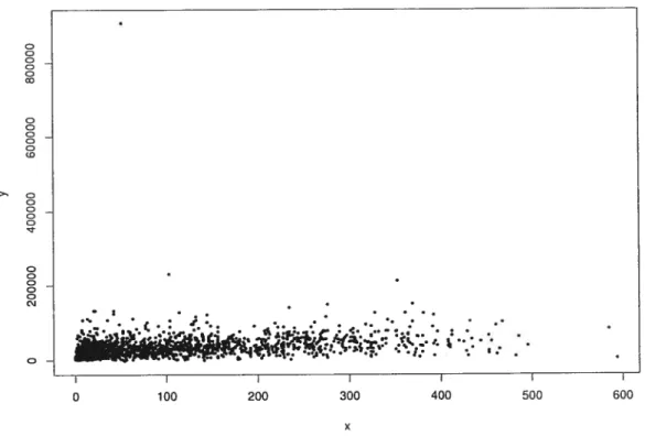
The third population is based on a random subsample of the $urvey ofLabor azid Income Dynamics, noted SL1D982. The survey vas conducted at Statistics Canada in 199$. For simplicity’s sake, only entries with no missing values were selected. The size of the subsample is N = 2000 and for our purpose this is assumed to be a population (the original sample

size of this survey is approximately 60,000). Taxable income (in thousands of dollars) is the target variable and the auxiliary variable is the duration in months of the current employment. From Figure 5, the linear relationship between taxable income and length of employment is Iess pronounced. However, the two variables do not appear to be independent. In Figure 6, the variable of interest exhibits a strong coefficient of skewness. We have drawn 500 samples from the SL1D982 population, according to SRS and P0 sampling plans. The sample sizes (expected sample size) n = 100 and n 200 were considered. For P0 sampling, the first order probabilities, lrk, k E U, were defined according to two rules. Under the first rule, the

lrk’swere created such that rk is approximately proportional to the variable ofinterest, that is taxable income (for the purpose of our study we assume that it is possible to create such lrk’s).

$ince some _Yk are negative in this population, we chose PIk Yk — min{yk, k E U} + 1 and

we defined 7rk = E(n)p1k/ >ZUP1k, where E(n) stands for the expected sample size, in our

case E(n8) = 100 and 200. Under the second rule, the ‘)rk’s were proportional to the entries

in Table 1. This means that for each k E U, there exists a factor ?2k, which is determined by the age-sex group of individual k. Then Jrk E(n)p2k/ P2k, where the factorsP2k are given in Table 1. The factors ?2k in Table 1 are based on a hypothetical sampling plan, in which we assume that these factors provide suitable size measures for the units in the various age-sex classes (see e.g., $iiindal et aÏ. (1992, p. 87)); for these units, more males than females are likely to be selected and, for both sexes, aduits in the 27 to 37 and 38 to 46 age range are more likely to be included in the sample.

In these three studies, we estimate the quartiles, that is the population parameters with a = 0.25, 0.5 and 0.75. Since the variables of interest display highly skewed distributions, it might be particulary interesting to study the quantile corresponding to a = 0.75, in addition

to the median and the first quartile. The next section describes the estimators included in the study.

27

Table 1: Factor _P2k by age and sex of individual k, in the $L1D982 population. Age

16—25 27—37 3$—46 17—69

Sex Male 3 6 5 4

Female 1 2 3 2

4.2 Estimators included n the empricaI study

Since one of our goals is to propose estimators with reasonable properties with respect to bias, variance and coverage rates of the conFidence intervals, we compare the new estimator defined by (9) based on the metric (2) to sorne of the popular quantile estimators proposed in the literature.

First, we include the simple design-based estimator based on the inversion of the estimator

Ê(t)

=

Z

dkH,5(t,Yk)/

Z

Qy,HT,c

Ê’().

(17)

The estimator (17) does not make use of auxiliary information. A possible variance estimator is

-2 A

{

Yk) -a

} {

Hy,s(y,ij,a, Yt) - a

}

where P/ ₌ d,, and confidence intervals can be calculated using

t’t1y),ÊYt2y)],

where

= — z1,2[Ç/{Py(Qy,)}]1/2,

(18) C2y = a + Z17/2[V{FY(QY,c)}1/. (19)

For more details, see Siirndal et aï. (1992, p. 202).

We also include in our empirical study the model-based estimator of Chambers and Dun stan (1986), which is motivated by a linear superpopulation model Yk = j3 +/3’xk+Ek, k E U,