HAL Id: hal-01931165
https://hal.insa-toulouse.fr/hal-01931165
Submitted on 23 Nov 2018HAL is a multi-disciplinary open access archive for the deposit and dissemination of sci-entific research documents, whether they are pub-lished or not. The documents may come from teaching and research institutions in France or abroad, or from public or private research centers.
L’archive ouverte pluridisciplinaire HAL, est destinée au dépôt et à la diffusion de documents scientifiques de niveau recherche, publiés ou non, émanant des établissements d’enseignement et de recherche français ou étrangers, des laboratoires publics ou privés.
J-Integrals Using the Submodeling Technique
Eduard Marenic, Ivica Skozrit, Zdenko Tonkovic
To cite this version:
Eduard Marenic, Ivica Skozrit, Zdenko Tonkovic. On the Calculation of Stress Intensity Factors and J-Integrals Using the Submodeling Technique. Journal of Pressure Vessel Technology, American Society of Mechanical Engineers, 2010, 132 (4), �10.1115/1.4001267�. �hal-01931165�
On the Calculation of Stress Intensity Factors and J-Integrals
Using the Submodeling Technique
Eduard Marenić, Ivica Skozrit and Zdenko Tonković* Faculty of Mechanical Engineering and Naval Architecture,
University of Zagreb, I. Lučića 5, 10000 Zagreb, Croatia
*Telephone: ++38516168450, Fax: ++38516168187, E-mail: [email protected]
Abstract
In the present paper, calculations of the stress intensity factor (SIF) in the linear elastic range and the J-integral in the elastoplastic domain of cracked structural components are performed by using the shell-to-solid submodeling technique to improve both the computational efficiency and accuracy. In order to validate the submodeling technique, several numerical examples are analyzed. The influence of the choice of the submodel size on the SIF and the J-integral results is investigated. Detailed finite element (FE) solutions for elastic and fully plastic J-integral values are obtained for an axially cracked thick-walled pipe under internal pressure. These values are then combined, using the General Electric/Electric Power Research Institute (GE/EPRI) method and the reference stress method (RSM), to obtain approximate values of the J-integral at all load levels up to the limit load. The newly developed analytical approximation of the reference pressure for thick-walled pipes with external axial surface cracks is applicable to a wide range of crack dimensions.
Keywords: finite element analysis, submodeling technique, stress intensity factor,
1. Introduction
Assessment of the structural integrity of cracked pressure vessel components fabricated from ductile materials can be performed by using elastoplastic fracture mechanics (EPFM) parameters and the limit load analysis. The most commonly used fracture parameter in EPFM is the J-integral. The calculation of the J-integral and the plastic limit load by using the incremental theory of plasticity requires a high computational effort [1, 2]. The J-integral estimation method based on the reference stress method [3] could reduce this effort since it only requires three basic data to be applied: the linear elastic fracture mechanics (LEFM) parameter (called the stress intensity factor) of the cracked component, the uniaxial true stress-strain curve of the material and the limit load able to produce its plastic collapse [4, 5, 6].
Due to fabrication defects, or damage in service, cracks exist generally in the areas of geometrical discontinuity of pressure vessel components where the stress concentration occurs. Therefore, cracks can be found near tubular joints, around weld toes. For a cracked tubular joint, the junction curve is a complicated space curve and the 3D meshing is very difficult and is even more demanding when the crack geometry has to be included. In order to calculate SIF one needs to use singular elements along the crack front, which generally leads to a 3D model. The number of elements required for a three dimensional FE model of the whole vessel volume, for example, would be very high, leading to extremely time-consuming solutions; therefore, the methodology would not be appropriate for design purposes. Furthermore, the accuracy of the numerical SIF results depends on the element type, mesh quality, mesh refinement, integration scheme and weld shape modeling. Elements near the crack front often have a high aspect ratio and, occasionally, some elements near the crack front are found to be badly distorted. This will influence SIF results significantly, and hence, in [7, 8, 9] a new method is
proposed to model the surface crack and to generate the FE mesh for cracked tubular joints. The tubular joint is divided into different, distinct zones which can greatly simplify the mesh generation process. For each zone, an FE mesh is generated separately and then merged in order to perform an analysis. The mesh quality can be controlled and improved, thus producing accurate and stable numerical results.
The line spring model introduced by Rice and Levy [10] reduces a 3D surface crack problem into a two-dimensional plate or shell theory problem. This approach is computationally inexpensive compared to fully 3D models and, within certain restrictions, provides acceptable accuracy [11, 12]. The main disadvantage of the model is that it does not take into account the curvature of the crack front and is not a good approximation near the ends where the crack intersects the free surface and its depth varies rapidly, due to the three-dimensional nature of the solution in such areas.
Recently, the submodeling technique has often been used in the FE numerical analysis to study in detail an area of interest in a model [13, 14, 15, 16, 17, 18]. Herein, the area of interest is the region of high stress caused by geometric discontinuities. The main idea of the submodeling technique is to perform a global (shell)-local (3D) transition. This approach gives an opportunity to make a local mesh refinement which brings considerable advantages. In the submodeling technique, the results from the global model are interpolated onto the nodes on the appropriate parts of the submodel boundary. A basic condition of the technique is that in the analysis the global model must define the submodel boundary response with sufficient accuracy. That means, when one is defining the submodel boundaries, in that area on the shell global model the displacement results must be accurate to a certain extent. In order to accomplish accuracy in the global model with a relatively coarse shell mesh, the submodel boundary must lie far enough from the intensive stress concentration. As the submodel
region has a finer mesh, the submodel can provide an accurate, detailed solution. Besides better accuracy, another advantage is that one can model a real problem more accurately by using a 3D submodel whose boundaries are driven by the shell submodel. This gain in accuracy is obtained because the 3D submodel can model cracks, welds, fillets, chamfers, etc. Unlike a large number of papers where the submodeling capability is used to obtain linear elastic SIF [13, 14, 15, 16, 17, 18], a very limited number of studies have been reported in the area dealing with the submodeling techniques in nonlinear EPFM. In that case, the loads are usually chosen so that the plastic zone around the crack tip is sufficiently small [1].
In the present investigation the submodeling capability is used to obtain a more accurate stress field at the crack tip in the linear elastic and nonlinear elastoplastic fracture mechanics problems. Efficiency and accuracy of the submodeling technique are demonstrated by several numerical examples. Thereby, the following is considered: a membrane with a semi-elliptical crack, a pipe with an external axial crack and a welded vessel-nozzle junction with a semi elliptical crack in the weld toe. The objective of this work is to determine the submodel size where nodal displacements for driven nodes of the submodel will be correctly interpolated from the results of the global model. Additionally, on the basis of detailed FE results obtained from the submodel analysis and using the reference stress approach [3], new reference pressure and J estimation equations are proposed for thick-walled pipes with external axial surface cracks under internal pressure. All computations have been performed within the FE software ABAQUS/Standard [19].
2. Elastic fracture mechanics analysis using submodeling
Three examples are used to check and verify submodeling in the SIF calculation with the results from the literature. The first example is a membrane with a semi-elliptical crack. In the second, a pipe with an external axial crack is analyzed. Finally, a semi-elliptical crack is included into the submodel of the vessel-nozzle junction.
2.1. A membrane with a semi-elliptical crack
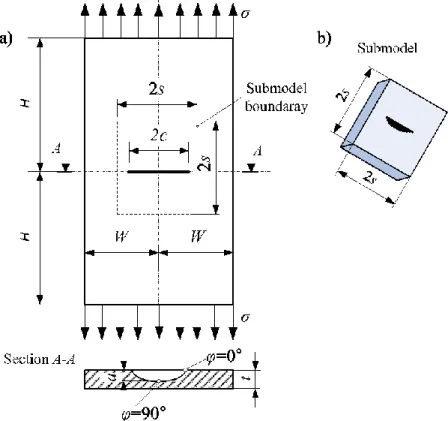
The first geometry to be analyzed is a membrane with a symmetric, centrally located, semi-elliptical crack loaded in Mode I by uniform tension applied to its top and bottom surfaces, as shown in Fig. 1. Employing symmetry, only one-quarter of the membrane is analyzed. The dimensions of the membrane relative to the membrane thickness t are as follows: the half-width W t/ 10, the half-length H t/ 25, the crack depth
/ 0.6
a t , and the crack half-length c t/ 0.8. A numerical solution for an uncracked membrane (global model) is obtained initially, where the membrane has been modeled without any crack. For shell-to-solid submodeling, the global model consists of 110 S8R shell elements, as shown in Fig. 2a. The results from the global analysis are interpolated on the boundary of the submodel with a crack included. The submodel consists of about 990 three-dimensional C3D20R elements (Fig. 2b). To avoid problems associated with incompressibility, the reduced integration is applied. In order to model strain singularity at the crack tip correctly, collapsed wedge-shaped elements are used.
Fig. 1 A membrane with a semi-elliptical crack subjected to tension: a) geometry,
dimensions and loading of the membrane, b) geometry of a submodel
Fig. 2 Meshes for semi-elliptical surface crack in a rectangular membrane: a)
one-quarter of the global (shell) model mesh without a crack, b) one-one-quarter of the submodel mesh with a semi-elliptical crack.
In order to be able to carry out the global analysis without a crack, and drive the cracked submodel with results from the global analysis, the submodel boundaries have to be chosen with good care. The submodel boundaries should be taken as close as
possible to the crack tip, but sufficiently far so that the stress field in the boundaries is completely unaffected by the crack. Herein, the submodel size 2s is chosen to be 2.5 times the size of the semi-elliptical crack, (i.e. the length 2 = (2.5...3) (2 )s c in Fig. 1) according to [15]. This example is simple and is used for the verification purpose. The assumption of a typical submodel size 2s is checked by modeling the whole membrane with three dimensional elements and with a crack included (Fig. 3). Numerical results show that stress distribution is altered only near the defect and it is enough to choose the submodel boundary such as 2 = 2.5 (2 )s c .
Fig. 3 A solid reference model of the cracked membrane
Verification of the numerical technique together with the validation of the submodeling technique in general and the submodel boundary selection are done by comparing numerical results with those obtained by Eq. (1) from API 579, Appendix C,
Compendium of stress intensity factor solutions [20]. According to the quoted reference,
SIF is estimated by using the following equation:
I ( m m b b) a K M M Q , (1)
where Mm and Mb are membrane and bending correction factors, respectively, and Q is
the elliptical integral approximated by
1.65 1 1.464 a Q c . (2)
A comparison of results for the SIF obtained numerically by using the submodeling technique and those obtained by using Eq. (1) is shown in Table 1. As one can see from the table, the results are in very good agreement. Good agreement shows that it is possible to perform the linear fracture mechanics analysis using the global-local technique. Although there are two steps that have to be carried out, this approach allows only the local mesh refinement with 3D elements together with singularity elements along the crack front. This kind of analysis where the refined 3D submodel is driven by a coarse global model enables a cost-effective analysis.
Table 1 Checking the validity of the submodeling technique
KI (MPa mm ) φ = 0° φ = 90°
API 579 [20] 127.8 156.4
submodeled FE analysis 123.4 152.8
2.2. A pipe with an external axial surface crack
The next step is to check the submodeling technique when a crack is introduced into a model with a more complex geometry, namely pressurized pipe. The surface-cracked pipe geometry and loading are shown in Fig. 4. Ri and Ro are the inner and the outer radius, while t denotes the wall thickness. The external surface crack is assumed to have a semi-elliptical shape described by a length 2c and a maximum depth a. An axial surface-cracked pipe is characterized by three non-dimensional parameters, i.e. Ri/t, c/a and a/t. Besides that, solutions for the limit pressure in literature are usually expressed in terms of a non-dimensional parameter ρ associated with the crack length c/ R t.
As evident from Fig. 4a, the internal pressure p is applied as a distributed load to the inner surface of the computational model. Since a pipe capped at both ends is considered, the corresponding axial tension force FπRi2p is applied at the ends of the model.
Fig. 4 A pipe with an external axial surface crack subjected to internal pressure: a)
geometry, dimensions and loading of the pipe, b) geometry of the submodel, c) geometry of the crack
As in the previous example, a numerical solution for an uncracked pipe is obtained initially (global model without a crack). Results obtained from the global analysis are interpolated on the submodel boundary and are used to drive the submodel with a crack included. A typical FE mesh applied in the analysis is shown in Fig. 5. Due to the symmetry of the problem, only a quarter of the pipe is considered in the modeling. The global model for the submodeling analysis is meshed with S8R shell elements as shown in Fig. 5a. The crack is not taken into consideration in the shell
model. The submodel is meshed by using three-dimensional C3D20R elements (see Fig. 5b). The overlay plot of the global model and the submodel is shown in Fig. 6.
Fig. 5 Typical FE meshes for a pipe: a) global (shell) model mesh without a crack, b)
submodel mesh with a semi-elliptical crack (Ri/t = 10, c/a = 10, a/t = 0.4, s/c = 2)
Fig. 6 Overlay plot of the global model and the submodel
In addition, a full three-dimensional C3D20R solid element mesh is considered for use as a reference solution (Fig. 7). The full solid element mesh in the crack-tip area is very similar to that used in the submodeling analyses. Moreover, both models have the same general characteristics. A difference exists in the modeling of pressure loading using the shell and continuum elements. The pressure loading is applied to the midsurface of the shell elements in contrast to the solid elements, where the pressure is accurately applied along the inside surface of the pipe.
Fig. 7 A solid reference model of the cracked pipe (Ri/t = 4, c/a = 10, a/t = 0.8)
A parametric study is performed, in which an inner radius-to-thickness ratio Ri/t takes the values of 4 and 10. Thereat, the wall thickness of the pipe t is held constant at a value of 1.625 mm. These values are chosen to represent a standard thick-walled pipes geometry (inner radius-to-thickness ratio Ri/t typically less than 10). Four different half crack length-to-crack depth ratios of c/a = 5, 10, 15 and 20, and crack depth-to-thickness ratios of a/t = 0.2, 0.4, 0.6 and 0.8 are considered. The actual dimension of the crack depth ranges from 0.325 mm to 1.3 mm and the crack length varies from 3.25 to
52 mm. Thus, a total of 32 cases are considered in the present investigation, as summarized in Table 2. In all analyses, the total length 2L of the pipe is chosen large enough so that the length would have a negligible effect on results (L/c ≥ 10). The material properties chosen are: E = 200 GPa, ν = 0.3, σy = 250 MPa where E is Young's modulus, ν Poisson's ratio and σy is the yield stress. The FE SIF solutions will be properly normalized in such a manner that the above mentioned choices do not affect the present results.
Table 2 FE models considered in the present analyses
FEM model no. Ri/t c/a a/t FEM model no. Ri/t c/a a/t
1 4 5 0.2 17 10 5 0.2 2 0.4 18 0.4 3 0.6 19 0.6 4 0.8 20 0.8 5 10 0.2 21 10 0.2 6 0.4 22 0.4 7 0.6 23 0.6 8 0.8 24 0.8 9 15 0.2 25 15 0.2 10 0.4 26 0.4 11 0.6 27 0.6 12 0.8 28 0.8 13 20 0.2 29 20 0.2 14 0.4 30 0.4 15 0.6 31 0.6 16 0.8 32 0.8
The linear-elastic FE computations yield the stress intensity factor K for an external axial surface crack in a pipe under internal pressure, which may be expressed by the following relation [21]: ) , , , ( m m t a t R F a t R p K (3)
where F(Rm/t,a/t,,) is a dimensionless function depending on the pipe and crack geometry and φ is the angle on an inscribed circle for locating a point on the crack, as shown in Fig. 4. The values of function F(Rm/t,a/t,,) obtained from the
submodeled analysis for the considered pipe geometry and the ratio of 2s/(2c) equal to 2.5 are tabulated in Table 3. As the SIF values reach the largest values at the deepest crack front location ( = π/2), only the results at that location are given.
Table 3 Dimensionless function F for the stress intensity factor
Rm/t 4 10
a/t c/a c/a
5 10 15 20 5 10 15 20 0.2 0.921 0.993 1.019 1.030 1.031 1.117 1.151 1.168 0.4 1.171 1.350 1.413 1.443 1.280 1.516 1.615 1.667 0.6 1.593 1.966 2.098 2.165 1.693 2.235 2.486 2.614 0.8 2.187 2.895 3.138 3.256 2.200 3.346 3.911 4.230
The variations of the difference in stress intensity factor with the increasing submodel size 2s from 2 to 12 times the size of the crack length 2c in the submodeled analysis are compared to the full solid (3D) element analysis in Fig. 8. The comparison is expressed as a percent difference that is defined as 100 ( KK3D) /K3D. It can be concluded from the results that for the pipe with an inner radius/thickness ratio of 10 a submodel size 2s equal to 2.5 times the size of the crack length 2c is sufficiently large for the linear elastic analysis (Fig. 8a). However, for very thick pipe with Ri/t = 4 the K value is stabilized for the ratio of 2s/(2c) equal to 5 (Fig. 8b). The error thereby introduced in the SIF value is up to around 1%.
Fig. 8 Dependence of the stress intensity factor on the submodel size:
In order to validate this assumption, the error analysis on the extracted submodel displacement boundary conditions is performed. In Figs 9 and 10 radial displacements distribution of inner surface of the pipe along a longitudinal and circumferential cross-section obtained from the FE submodeling approach is presented and compared to the full 3D solid and shell models. Responses in hoop stresses are plotted in the Figs 11 and 12. The results given in this graphs refer to R ti/ 10, c a/ 10, a t/ 0.4, t = 1.625 mm, s c/ 2 and 3. As may be observed from Figs 9 to 12, the results obtained by the submodel ratio of 2s/(2c) equal to 2 deviate significantly. On the other hand, for the submodel ratio of 2s/(2c) equal to 3 the displacements and hoop stresses show very little difference between the two analysis.
Fig. 9 Radial displacements distribution of inner surface of the pipe along a
Fig. 10 Radial displacements distribution of inner surface of the pipe along a
circumferential cross-section (R ti/ 10)
Fig. 11 Hoop stresses distribution of inner surface of the pipe along a longitudinal
Fig. 12 Hoop stresses distribution of inner surface of the pipe along a circumferential
cross-section (R ti/ 10)
As mentioned before, the same pressure is applied on the inner radius of the 3D solid FE model as on the mean radius of the shell model (Fig. 13a). For very thin pipes this doesn’t make a practical difference, but for pipes studied here the membrane displacement for pipes with ratio R ti/ 10 and R ti/ 4 is too high in shell model for 3.4% and 8.9% respectively. For the hoop stress this difference is 4.8% and 11.4% for ratio 10 and 4 respectively. In order to study this effect, in Figs 9 to 12 the results for the radial displacements and hoop stresses are also presented for the submodel without crack. Internal pressure acting on the internal surface of the 3D submodel results in smaller load than in the shell’s mid surface. Due to smaller load on inner surface of 3D submodel without crack, displacement distribution (Fig. 9) underestimate global, shell membrane displacement which is used as a submodel boundary condition. This displacement mismatch causes submodel bending shown in Figs 13a and b. Besides shell and submodel without crack, in Fig 13a deformed configuration of full 3D model without crack is shown. Even though the radial displacement of the global model are too high and causes submodel bending, when crack is introduced in submodel firstly
finally SIF obtained by submodeling analysis (driven with higher global displacements) are not overestimated compared with cracked full 3D model. Described effect of displacement mismatch and submodel bending and it’s influence to hoop stress is more obvious in thicker pipes. For pipe with radius-to-thickness ratio Ri/t = 4, in order to have equivalent submodeling analysis to full 3D, one have to build bigger submodel (Fig. 14), say s/c = 4. In addition it can be concluded from Figs 9. to 12. that the submodel size in circumferential direction may be smaller than in the longitudinal. So for the pipe with ratio of Ri/t = 10 optimum submodel size in circumferential direction is
circ / 2
s c , and in longitudinal
long / 3
s c .
Fig. 13 Submodel and full 3D model without crack under the same pressure:
a) schematic representation of deformed configurations, b) deformed configuration of the submodel
Fig. 14 a) Hoop stresses distribution of inner surface of the pipe along a longitudinal
cross-section (R ti/ 4,c a/ 5, a t/ 0.4, t = 1.625 mm, s c/ 3 and 4), b), c) details A and B
The values of the dimensionless function F for the stress intensity factor obtained by the submodeled analysis are also compared with the solutions obtained by [21] for the selected values of t/Ri = 0.1, a/c = 0.2, 0.4, 1.0, a/t = 0.2, 0.5, 0.8 and s/c = 3 (Fig. 15). The results compare satisfactorily, while only slight differences in less than 6% of the F values are exhibited. These differences could arise from the fact that the solutions obtained by Raju and Newman are given for the model with two diametrically located cracks. Additionally, the differences occur due to the numerical inaccuracy of the results in [21], as also shown in [5].
Fig. 15 A comparison of the dimensionless function F for the stress intensity factor
between the present work and the published solutions obtained by Raju and Newman [21]
2.3. A welded vessel-nozzle junction with a semi-elliptical crack in weld toe
In the above examples, submodeling has been verified as an efficient, cost-effective approach in the calculation of fracture mechanics parameters in simpler examples; it is justified to use the same procedure for a real welded vessel-nozzle junction. The accurate calculation of stress intensity factors for semi-elliptical weld toe cracks (Fig. 16) is a rather difficult task because the geometry of the joint with crack is extremely complex and, hence, difficult to model.
In general, a major problem in using solid elements lies in generating an adequate mesh for accurate solutions (for example to create a good 3D, hexahedral mesh). This problem is partially solved when the global-local approach is used because just part of interest is modeled as a solid. Usually, the geometry of this relatively small submodel (with respect to the whole global model) can be divided into considerably simpler cells which can be meshed easily. A similar approach is used in [7, 8, 9], as described in the introduction section of the paper, where the joint is divided into zones, meshed zone by zone, and afterwards merged together for analysis.
The computational model of the considered junction is shown in Fig. 16. Weld joints are marked with numerals from 1 to 3. In the present analysis only weld 1 is taken into consideration. The semi-elliptical surface crack is introduced into the model near the weld toe of the vessel-nozzle junction, where a high stress concentration exists. In [20], this type of crack which is located on the outer surface is labeled as type D.
Fig. 16 Computational model of the vessel-nozzle junction with a crack in the weld toe
A nozzle of the inner diameter d2 = 43.9 mm and the wall thickness t2 = 8.7 mm is attached to a vessel which has an inner diameter of d1 = 1220 mm, wall thickness of t1 = 15 mm, and is assumed to be very long (2L = 8000 mm). Length and depth of the external semi-elliptical crack are 2c = 24 mm and a = 6 mm, respectively. Considering symmetry again, only a half of the assembly is modeled by a FE mesh. The nozzle, vessel and joint are assumed to be made of the same material with E = 200 GPa and = 0.3. Again, the global shell model is meshed with S8R elements, and the submodel is meshed with C3D20R elements (see Figs 17a, b and c). The submodeling technique enables the easy modeling of a real geometry (welds, chamfers, etc.) because it is possible to use a global model, consisting of a coarse mesh of shell elements without a weld, to drive a more complex local model with an explicit weld. Accordingly, the crack and the weld 1 are not taken into account in the shell model. The 3D submodel mesh models the crack and the ring of welded material accurately to include the welded joint 1. In the considered example, the vessel-nozzle junction is subjected to the internal pressure of 1 MPa.
Fig. 17 Typical FE meshes for a vessel-nozzle junction: a) global (shell) model mesh
without a crack, b) a junction detail of the global model, c) the submodel mesh with a semi-elliptical crack in the weld toe, d) 3D model mesh without a crack
In order to have accurate results from the global (shell) model, the optimal submodel size for the vessel-nozzle junction (Fig. 17c) is selected on the basis of the error analysis on the extracted submodel displacement boundary conditions. In Fig. 18 variations of the difference in radial displacements distribution of mid surface along a longitudinal and circumferential cross-section of the pressure vessel obtained from the shell model are presented and compared to the full 3D solid FEA. Thereby, the crack and the weld are not taken into account in the shell model (Fig. 17a and b). On the other hand, the 3D model mesh models the crack and the ring of welded material accurately to
that is defined as 100 ( ur,shellur,3D) /ur,3D. It can be concluded from the results that a submodel size s equal to 10 times the size of the wall thickness t1 is sufficiently large for the SIF analysis. The error thereby introduced in the radial displacement values is up to around 1.5%. It should be noted that this is true when the crack in the weld toe is small. Additionally it can be concluded from Fig. 18 that the submodel size in circumferential direction may be somewhat smaller than in the longitudinal.
Fig. 18 Variations of the difference in radial displacements distribution of mid surface
along a longitudinal and circumferential cross-section of the pressure vessel obtained from the shell model and the full 3D solid FEA
The numerical results and submodeling technique are verified with the results from [20]. Using API code [20], KI can be calculated by means of the following equation: I 0 ( , ) ( ) a K
h x a x dx, (4)where h(x, a) is the weight function, and σ(x) is the stress normal to the crack plane but when the junction is in uncracked state. Coordinate x is the through-thickness distance measured from the outer surface of the vessel. A comparison between numerical results
obtained by using the submodeling technique and the results calculated by means of Eq. (4) is shown in Table 4. In this table 0 represents the right point (far from the weld), 90 the deepest point and 180 defines the left point (close to the weld). The results are in good agreement, so it is obvious that the submodeling technique is an efficient technique, especially for complicated geometries like in this case.
Table 4 Comparison of the SIF results between the present work and [20]
KI (MPa mm ) φ = 0° φ = 90° φ = 180°
API 579 [20] 270.2 365.6 -
submodeled FE analysis 268.8 354.2 256.6
3. Elastoplastic fracture mechanics analysis using submodeling
In the previous section, the SIF calculation is performed by using the FE submodeling technique. In this section, the intention is to verify the submodeling technique in the elastoplastic Jep-integral evaluation for a pipe with an external axial surface crack considered in the section 2.2.
3.1. J estimation by the GE/EPRI method
In the structural integrity assessment procedures the values of the elastoplastic Jep-integral are obtained by using the deformation theory of plasticity, where the stress-strain response in the FE analyses is described by the well-known Ramberg-Osgood model in the following form:
0 y y n . (5)
In Eq. (5), 0 denotes the associated reference strain 0 y/ E while the values and
developed by the General Electric/ Electric Power Research Institute (GE/EPRI) , the total crack driving force Jep can be divided into elastic, Jel, and plastic, Jpl, parts, as
ep el pl
J J J . (6)
The elastic component of the Jep-integral, Jel, can be estimated from the SIF with a plasticity correction [4] as follows:
2 e el , K a J E , (7)where E' E for the plane stress (0) and E'E/(12) for plane strain conditions (0). ae is the effective crack length defined by the relation
2 e 2 y 1 1 1 6 1 1 / L n K a a n p p . (8)In Eq. (8), pL is the plastic limit pressure that produces the plastic collapse of the surface cracked pipe for a rigid-plastic, non-hardening material with the yield stress y [22, 23]. The empirical expression for the estimation of the plastic limit pressure for the considered pipe and crack geometry in terms of the non-dimensional crack configuration parameters a/t and ρ was proposed by the authors [23, 24]. The basic equations are compiled in Table 5. In the previously mentioned references, extensive FEAs have been performed to validate the results of the plastic limit pressure by comparing the computed values with the existing solutions [2, 25, 26]. As shown, the analytical approximation of the plastic limit pressure for thick-walled pipes is applicable to a wide range of crack dimensions.
Table 5 Basic equations for the estimation of the plastic limit pressure [23]
Plastic limit pressure: ) , / ( 0 L p P a t p . (9)
Limit pressure of an un-cracked thick-walled pipe based on the Von Mises yield criterion:
i o y 0 ln 3 2 R R p . (10)
Dimensionless parameter which is a function of crack configuration parameters a/t and ρ:
2 2 1 1 t a P t a P P , where P10.1353120.3515170.06717320.0049543, 3 2 20.1234880.0110680.009342 0.001921 P . (11)
Nonlinear FE analysis has been performed to evaluate the J-integral. The values of the
J-integral are computed around 5 contours surrounding the crack tip. The result from the
1st contour closest to the crack tip is discarded, and the J-integral value is the average of all the values obtained on the 2nd to 5th contour. The submodeling capability is now used to analyze the crack-tip region when the material behavior is elastoplastic. In the present investigation, the FE solutions for elastic and fully plastic J-integral values are first obtained for an axially cracked pipe, and are then combined, using GE/EPRI and the reference stress method [3], to obtain approximate values of the Jep-integral at all load levels up to the limit load. In order to validate the model, the mesh convergence is investigated to describe the fully plastic flow field accurately. A total of 160 cases are considered. Herein, values of the strain hardening index n are systematically varied: n = 3, 5, 7 and 10, while parameter is fixed to = 1.
Additionally, in order to investigate the dependence of the Jep-integral results on the submodel size, ten different submodel size-to-crack length ratios of 2s/(2c) = 2, 3, 4, 6, 8, 10, 12, 14, 16 and 18 are considered. The results for the Jep-integral values at the deepest crack front location (φ = π/2), as functions of applied pressure, from the submodeled analyses are compared to the full solid (3D) element mesh. Figure 19
plastic zone size is less than about 10% of the crack length, small-scale yielding conditions exist around the crack tip. In that case, the far-field elastic region is not affected by the plastic zone. In our case, this will be true for the relatively small pressures that cause the sufficiently small plastic zones. As may be observed from Fig. 19, with a further pressure increase, larger plastic strains occur on the model and a submodel size 2s equal to 2.5 times the size of the crack length 2c is not sufficiently large for analysis. For the load levels of up to 180% of limit load, the J value is stabilized for the ratio of 2s/(2c) equal to 4. It is valid only for the pipe with R ti/ 10 (Fig. 19a). However, for very thick pipe with Ri/t = 4 there is no significant stabilization of the J value (Fig. 19a). Since the differences in results are generally lower for submodel size of s/c = 4 then for other submodels, the submodel size of s/c = 4 can be taken as relevant for submodeled elastoplastic analysis of cracked pipes. For this reason, submodeled analyses for calculation of the J-integral are performed by using the submodel size-to-crack length ratio of 4.
From Fig. 19 it can also be concluded that the difference between the results obtained by submodeled and full solid element analysis becomes larger with increasing pressure. Thus, for the larger submodels the maximum differences in results are 1.3% for pipe with Ri/t = 10 and 4% for Ri/t = 4. These differences are connected with the modeling of the spread of the plastic zone through the thickness of the pipe and different finite element formulations of shell and solid elements applied to perform submodeled and full solid element analysis. In the present example, the global model for the submodeling analysis is meshed with S8R thick shell elements (Fig. 5a) with five integration points through the thickness. On the contrary, the full solid element analysis is performed by using a single C3D20R element with reduced integration (2x2x2) through the thickness (Fig. 7) further away from the crack.
Fig. 19 Dependence of the Jep-integral results on the submodel size: a) R ti/ 10, /c a10, a t/ 0.4, b) R ti/ 4, /c a5, a t/ 0.4
Following reference [27], the plastic part of Jep-integral, Jpl, for semi-elliptical surface cracked pipes is given by
1 2 y i pl 1 L , , , , , n p R a c J t a h n E p t t a (12)where h1 is the dimensionless plastic influence function which depends on the crack and pipe geometry. In order to obtain the values of the function h R t a t c a1
i/ , / , / ,
, the plastic part of Jep integral is determined bypl_FE FE el
J J J . (13)
It is to be noted that the value of h1 depends on the load magnitude, as shown in Fig. 20. Since the power-law part of Eq. (5) describing the material behavior during the loading process is dominant at sufficiently large loads, the values of h1(a/t, c) at high loads should be taken from appropriate diagrams [5]. The values of h1(a/t, c) obtained from the submodel analysis for the considered pipe geometry and ratio of 2s/(2c) equal to 4 at the deepest crack front location ( / 2) are presented in Table 6. Thus, according to the GE/EPRI method, the Jep-integral can be estimated by using Eqs (5) to (13) and the data given in Tables 3 and 6.
Fig. 20 Dependence of the plastic influence h1-function on the load magnitude (Ri/t 4,c/a5): a) a/t0.2, b) a/t0.6
Table 6 Values of the plastic influence h1-functions Ri/t c/a a/t n Ri/t c/a a/t n 3 5 7 10 3 5 7 10 4 5 0.2 1.358 1.737 2.020 2.370 10 5 0.2 1.521 1.872 2.161 2.540 0.4 5.563 7.228 8.357 9.482 0.4 6.424 8.254 9.739 11.386 0.6 15.943 18.571 19.581 20.009 0.6 19.903 23.354 25.421 26.766 0.8 37.093 38.727 38.132 34.822 0.8 51.712 57.183 60.255 59.333 10 0.2 1.570 2.075 2.449 2.868 10 0.2 1.803 2.299 2.688 3.174 0.4 6.556 8.604 9.708 10.356 0.4 8.395 11.071 12.818 14.223 0.6 16.592 17.815 17.681 17.112 0.6 26.156 29.434 31.093 32.007 0.8 29.855 27.973 25.438 21.583 0.8 57.742 58.603 60.943 60.396 15 0.2 1.581 2.102 2.483 2.879 15 0.2 1.865 2.405 2.819 3.324 0.4 6.312 8.256 9.146 9.504 0.4 8.678 11.579 13.262 14.492 0.6 14.925 15.394 14.875 14.002 0.6 25.213 27.009 27.327 27.030 0.8 27.514 27.749 27.309 25.622 0.8 47.198 45.301 45.762 43.527 20 0.2 1.536 2.033 2.392 2.743 20 0.2 1.850 2.388 2.792 3.272 0.4 5.958 7.772 8.554 8.803 0.4 8.387 11.241 12.750 13.676 0.6 14.133 14.476 14.087 13.490 0.6 23.587 24.393 24.021 23.255 0.8 22.731 22.968 22.615 21.040 0.8 43.821 42.614 44.701 45.104
A summary of the typical computational requirements for the full 3D solid and submodeled elastoplastic FE analysis of the pipe with an external axial surface crack is given in Table 7. The results given in this table refer to R ti/ 10, c a/ 10, a t/ 0.4,
/ 4
s c . All computations were done on the PC Intel Core 2 Quad processor with 4x2.4GHz (4GB RAM). The computational cost in CPU seconds of the submodeled analysis is approximately 58% of the CPU time of the full 3D solid analysis. This gain in CPU time gets more and more obvious for complex geometry of the cracked component. The global shell model with 3D submodel has 72% of the total number of degrees of freedom required for the full 3D solid model. The size of the data library for the submodeled analysis is approximately 60% of the size of the data library required for the analysis of the full 3D solid model. The size of the model is greatly reduced by adopting the submodeled analysis with negligible loss of the results.
Table 7 Summary of computational requirements for the elastoplastic analysis of the
pipe with an external axial surface crack
Model
Measures of computational effort Total number of
degrees of freedom CPU s
Size of data library, (megabytes)
Full 3D solid model 76461 686 38.0
Global shell model +
3D submodel 55052 398 22.7
3.2. J estimation by the reference stress method
As presented, the J estimation based on GE/EPRI method requires the Ramberg-Osgood coefficient and strain hardening index as basic input to represent material tensile data. The disadvantage here is that Ramberg-Osgood fitting of the stress-strain curve can be seriously inaccurate, leading to inaccuracy in the estimated J [5, 28]. The limitation of this method is that plastic influence functions should be found, which requires detailed 3D elastoplastic FE analyses [5, 27, 28, 30]. Thereby, the solutions for plastic influence functions, available in fracture mechanics handbooks, are limited to a relatively simple geometrical configuration and dimensions of both the crack and the structural element under simple loading conditions. For more realistic and complex crack geometries and loading conditions, the GE/EPRI J estimation method is impractical for engineering application. Additionally, Kim et al. [5] and Chattopadhyay et al. [28] showed that GE/EPRI method over-estimates the plastic J with respect to the incremental plasticity FE solutions. For application to general stress-strain laws, the Jep estimation equation is now re-formulated by using the reference stress method in the form [3, 4, 29]
2
ref ref ref
ep el ref y ref 1 2 E J J E , (14)
where ref denotes the reference stress, ref ( /p pref)y, and ref is the reference strain at ref, determined from the true-stress strain data, while pref stands for the reference pressure. Unlike the conventional reference stress method [3, 4] where the reference stress is defined by using the plastic limit load, the enhanced reference stress method (ERSM), proposed in [5], defines the reference stress with the optimized reference load. The optimized reference load is found to give the best estimates of J. Detailed information on the proposed method can be found in Ref. [5, 30]. Based on the FE results from the submodeled analyses and the mentioned enhanced reference stress concept, the empirical expression for the estimation of the optimized reference pressure
pref for pipes with external axial semi-elliptical surface cracks is derived as follows:
1 1 1 ref 0 1 ( 1) / , ( ) n L h n p p p S a t h n , (15)where pL and p0 are defined by Eqs (9) and (10). S is the dimensionless factor which is a function of non-dimensional crack configuration parameters a/t and ρ given by:
2 1 2 1 a a S S S t t , (16) where 2 3 1 2 3 2 0.92351 0.18551 0.058677 0.00539 , 1.066525-0.16797 0.00265 0.002479 . S S (17)
The reference stress-based Jep estimation (Eq. 14) is compared with the GE/EPRI solutions as well as with FE results where the non-linear material behavior is modeled by using incremental plasticity with the von Mises yield function, together with the
for the austenitic steel 08X18H10T that corresponds to the German grade 1.4541 (equivalent to AISI 321), used in the analysis and determined experimentally in a standard tensile test, are taken from [31]. The basic material parameters are summarized in Table 8 for 300 C. Figure 21 displays the engineering stress-strain curve (σe, εe).
Table 8 Mechanical properties of the austenitic steel 08X18H10T at 300°C [31]
Temperature, T (C) Modulus, E (GPa) Yield stress, σy (MPa) Ultimate stress, σu (MPa) n 300 184 160 420 1.375 4.01
Fig. 21 Engineering stress-strain curves of the 08X18H10T steel at 300 C [31]
The true stress and strain values (σt, εt) used in the incremental plasticity analysis are determined by the following relationships:
e
e t 1 , (18)
e
t ln 1 . (19)The values of both the engineering terms and true terms are shown in Table 9. The data is given up to the ultimate tensile stress level (25% of strain). After this specified point, the response is assumed to be perfectly plastic.
Table 9 Material data of the austenitic steel 08X18H10T at 300 C [31] Engineering stress, σe (MPa) Engineering plastic strain, εe,pl True stress σt (MPa)
True plastic strain, εt,pl 160 0.000 160 0.000 184 0.006 186 0.006 223 0.016 226 0.016 251 0.026 258 0.026 283 0.042 295 0.041 312 0.059 330 0.057 344 0.079 371 0.076 365 0.098 401 0.094 413 0.198 495 0.181 420 0.248 524 0.221
As may be observed from Fig. 22, excellent agreement of the two RSM and FE solutions is exhibited. On the other hand, the results obtained by the GE/EPRI deviate significantly.
Fig. 22 Comparison of FE and GE/EPRI J results with the proposed reference
stress-based J estimations (Rm/t = 4.8, c/a = 2.08, a/t = 0.8)
Conclusions
In the present investigation the shell-to-solid submodeling capability is used to obtain a more accurate crack tip stress field in the linear elastic and nonlinear elastoplastic fracture mechanics problems. Computational efficiency of the submodeling technique
for SIF calculation is demonstrated by three numerical examples. The first one is a membrane with a semi-elliptical crack under tension, and the other one is a pressurized thick-walled pipe with a finite external axial surface crack. These two examples are used to verify submodeling in the SIF calculation with the results from the literature. The influence of the choice of the submodel size on the SIF results is investigated. Together with the submodel size study, the effect of the error caused by the same pressure defined on the inner radius of the 3D solid FE model as on the mean radius of the shell model is analyzed. It is concluded that the choice of the submodel can compensate for pressure definition error and that there is no need for pressure correction. In accordance with literature results [15], the study also concluded that a submodel size equal to 2.5 times the size of the crack length is sufficiently large for the linear elastic analysis. Finally, the semi-elliptical surface crack is introduced into the real model near the weld toe of the vessel-nozzle junction, where a high stress concentration exists. The submodeling technique, based on the transition from the global shell model to the three-dimensional submodel discretized with a finer mesh of elements, is proven to be very efficient for this purpose.
As the last example, in order to verify the submodeling technique in the elastoplastic J-integral evaluation, a thick-walled pipe with an external axial surface crack under internal pressure is considered. The dependence of the J-integral results on the submodel size is investigated for the load levels up to the limit load. In addition, the submodel mesh convergence is analyzed to describe the fully plastic flow field accurately. It is shown that, unlike the LEFM problems, the submodel size must be minimum 4 times the size of the crack length. Based on the FE results from the submodel analyses and by using the enhanced reference stress concept, an empirical expression for the estimation of the optimized reference pressure for cracked pipes is
proposed. The proposed SIFs, J-integral and the analytical approximation of reference pressure for the considered pipe and crack geometries are very useful tools for assessing the integrity of pressurized pipes.
Acknowledgements
The authors express their gratitude to the Ministry of Science, Education and Sports of the Republic of Croatia for their financial support.
References:
[1] Simha, N.K., Fischer, F.D., Shan, G.X., Chen, C.R. and Kolednik, O., 2008, “J-integral and crack driving force in elastic–plastic materials,” Journal of the Mechanics and Physics of Solids, 56(9), 2008, pp. 2876-2895.
[2] Kim, Y. –J., Shim, D. –J., Huh, N. –S., and Kim, Y. –J., 2002, “Plastic Limit Pressures for Cracked Pipes Using Finite Element Limit Analyses,” International Journal of Pressure Vessels and Piping, 79, pp. 321–330.
[3] Ainsworth, R. A., 1984, “The Assessment of Defects in Structures of Strain Hardening Material,” Engineering Fracture Mechanics, 19, pp. 633-642.
[4] R6, 2001, “Assessment of the Integrity of Structures Containing Defects”, revision 4. British Energy Generation Ltd.
[5] Kim, Y. J., Kim, J. S., Park, Y. J., and Kim, Y. J., 2004, “Elastic-Plastic Fracture Mechanics Method for Finite Internal Axial Surface Cracks in Cylinders,” Engineering Fracture Mechanics, 71, pp. 925-944.
[6] Moreno, J., and Valiente, A., 2008, “Assessment of the Reference Stress Method for J-Integral Estimation of Cracked Riveted Beams of an Old Wrought Iron,” Engineering Failure Analysis, 15, pp. 194-207.
[7] Chiew, S. P., Lie, S. T., Lee, C. K., and Huang, Z. W., 2001, “Stress Intensity Factors for Surface Crack in a Tubular T-Joint,” International Journal of Pressure Vessels and Piping, 78, pp. 677-685.
[8] Lie, S. T., Lee, C. K., and Wong, S. M., 2003, “Model and Mesh Generation of Cracked Tubular Y-Joints,” Engineering Fracture Mechanics, 70(2), pp. 161-184. [9] Lie, S. T., Lee, C. K., Chiew, S. P., and Shao, Y. B., 2005, “Mesh Modelling and
Analysis of Cracked Uni-Planar Tubular K-Joints,” Journal of Constructional Steel Research, 61, pp. 235-264.
[10] Rice, J.R. and Levy, N., 1972, “The part-through surface crack in an elastic plate,” Transactions of the ASME, Journal of Applied Mechanics, 39, pp. 185–194. [11] Parks, D.M., 1981, “The inelastic line-spring: estimates of elastic–plastic fracture
mechanics parameters for surface cracked plates and shells,” Transactions of the ASME, Journal of Pressure Vessel Technology, 103, pp. 246–254.
[12] Berg, E., Skallerud, B. and Thaulow, C., 2008, “Two-parameter fracture mechanics and circumferential crack growth in surface cracked pipelines using line-spring elements,” Engineering Fracture Mechanics, 75(1), pp. 17-30.
[13] Haryadi, S. G., Kapania, R. K. and Haftka, R. T., 1998, “Global/local analysis of composite plates with cracks,” Composites Part B: Engineering, 29(3), pp. 271-276.
[14] Bakuckas Jr., J.G., 2001, “Comparison of boundary correction factor solutions for two symmetric cracks in a straight-shank hole,” Engineering Fracture Mechanics, 68(9), pp. 1095-1106.
[15] Diamantoudis, A., and Labeas, G., 2005, “Stress Intensity Factors of Semi-Elliptical Surface Cracks in Pressure Vessels by Global-Local Finite Element Methodology,” Engineering Fracture Mechanics, 72, pp. 1299-1312.
[16] Levy, C., Perl, M. and Kotagiri, S., 2008, “The Combined Stress Intensity Factors of Multiple Longitudinally Coplanar Cracks in Autofrettaged Pressurized Tubes Influenced by the Bauschinger Effect,” Transactions of the ASME, Journal of Pressure Vessel Technology, 130 (3), 031208.
[17] Liu, Y., Stratman, B. and Mahadevan, S., 2006, “Fatigue crack initiation life prediction of railroad wheels,” International Journal of Fatigue, 28(7), 2006, pp. 747-756.
[18] Mikhaluk, D.S., Truong, T.C., Borovkov, A.I., Lomov, S.V. and Verpoest, I., 2008, “Experimental observations and finite element modelling of damage initiation and evolution in carbon/epoxy non-crimp fabric composites,” Engineering Fracture Mechanics, 75(9), pp. 2751-2766.
[19] Hibbitt, Karlsson & Serensen, Inc., 2008, “ABAQUS/Standard. User's Guide and Theoretical Manual,” Version 6.8.
[20] API 579, 2000, “Recommended practice for fitness-for-service,” American Petroleum Institute, Issue 6.
[21] Raju, I. S., and Newman, J. C., 1982, “Stress-Intensity Factors for Internal and External Surface Cracks in Cylindrical Vessels,” Transactions of the ASME, Journal of Pressure Vessel Technology, 104, pp. 293-298.
[22] Miller, A. G., 1988, “Review of Limit Loads of Structures Containing Defects,” International Journal of Pressure Vessels and Piping, 32, pp. 197-327.
[23] Tonković, Z., Skozrit, I., and Alfirević, I., 2008, “Influence of Flow Stress Choice on the Plastic Collapse Estimation of Axially Cracked Steam Generator Tubes,” Nuclear Engineering and Design, 238, pp. 1762-1770.
[24] Tonković, Z., Skozrit, I., and Sorić, J., 2005, “Numerical Modelling of Deformation Responses of Cracked Tubes,” Transactions of FAMENA, 29(1), pp. 31-38.
[25] Carter, A. J., 1991, “A Library of Limit Loads for FRACTURE TWO,” Internal Report TD/SID/REP/0191, Nuclear Electric.
[26] Staat, M., 2005, “Local and Global Collapse Pressure of Longitudinally Flawed Pipes and Cylindrical Vessels,” International Journal of Pressure Vessels and Piping, 82, pp. 217-225.
[27] Kumar, V., and German, M. D., 1988, “Elastic-Plastic Fracture Analysis of Through-Wall and Surface Flaws in Cylinders,” EPRI Topical Report. NP-5596, Electric Power Research Institute, Palo Alto, CA.
[28] Chattopadhyay, J., 2006, “Improved J and COD estimation by GE/EPRI method in elastic to fully plastic transition zone,” Engineering Fracture Mechanics, 73, pp. 1959–1979.
[29] Miller, A. G., and Ainsworth, R. A., 1989, “Consistency of Numerical Results for Power-Law Hardening Materials and the Accuracy of the Reference Stress Approximation,” Engineering Fracture Mechanics, 32, pp. 237-247.
[30] Kim, Y., Huh, N., Park, Y., and Kim, Y., 2002, “Elastic–Plastic J and COD Estimates for Axial Through-Wall Cracked Pipes,” International Journal of Pressure Vessels and Piping, 79, pp. 451-464.
[31] Norms, 1989, “Norms for the Calculation of Strength of the Equipment and the Pipelines of Nuclear Power Installations (PNAE G-7-002-86),” Regulatory Authority for the Control of Nuclear Power of the USR-Moscow, Energoatomizdat (in Russian).
Figure captions:
Fig. 1 A membrane with a semi-elliptical crack subjected to tension: a) geometry,
dimensions and loading of the membrane, b) geometry of a submodel
Fig. 2 Meshes for semi-elliptical surface crack in a rectangular membrane: a)
one-quarter of the global (shell) model mesh without a crack, b) one-one-quarter of the submodel mesh with a semi-elliptical crack.
Fig. 3 A solid reference model of the cracked membrane
Fig. 4 A pipe with an external axial surface crack subjected to internal pressure: a)
geometry, dimensions and loading of the pipe, b) geometry of the submodel, c) geometry of the crack
Fig. 5 Typical FE meshes for a pipe: a) global (shell) model mesh without a crack, b)
submodel mesh with a semi-elliptical crack (Ri/t = 10, c/a = 10, a/t = 0.4, s/c = 2)
Fig. 6 Overlay plot of the global model and the submodel
(Ri/t = 10, c/a = 10, a/t = 0.4, s/c = 2)
Fig. 7 A solid reference model of the cracked pipe (Ri/t = 4, c/a = 10, a/t = 0.8)
Fig. 8 Dependence of the stress intensity factor on the submodel size:
Fig. 9 Radial displacements distribution of inner surface of the pipe along a
longitudinal cross-section
Fig. 10 Radial displacements distribution of inner surface of the pipe along a
circumferential cross-section
Fig. 11 Hoop stresses distribution of inner surface of the pipe along a longitudinal
cross-section
Fig. 12 Hoop stresses distribution of inner surface of the pipe along a circumferential
cross-section
Fig. 13 Submodel and full 3D model without crack under the same pressure:
a) schematic representation of deformed configurations, b) deformed configuration of the submodel
Fig. 14 a) Hoop stresses distribution of inner surface of the pipe along a longitudinal
cross-section (R ti/ 4,c a/ 5, a t/ 0.4, t = 1.625 mm, s c/ 3 and 4), b), c) details A and B
Fig. 15 A comparison of the dimensionless function F for the stress intensity factor
between the present work and the published solutions obtained by Raju and Newman [21]
Fig. 16 Computational model of the vessel-nozzle junction with a crack in the weld toe
(type D according to [20])
Fig. 17 Typical FE meshes for a vessel-nozzle junction: a) global (shell) model mesh
without a crack, b) a junction detail of the global model, c) the submodel mesh with a semi-elliptical crack in the weld toe
Fig. 18 Variations of the difference in radial displacements distribution of mid surface
along a longitudinal and circumferential cross-section of the pressure vessel obtained from the shell model and the full 3D solid FEA
Fig. 19 Dependence of the Jep-integral results on the submodel size: a) i/ 10, / 10, / 0.4
R t c a a t , b) R ti/ 4, /c a5,a t/ 0.4
Fig. 20 Dependence of the plastic influence h1-function on the load magnitude (Ri/t 4,c/a5): a) a/t0.2, b) a/t0.6
Fig. 21 Engineering stress–strain curves of the 08X18H10T steel at 300 C [31]
Fig. 22 Comparison of FE and GE/EPRI J results with the proposed reference
Table captions:
Table 1 Checking the validity of the submodeling technique
Table 2 FE models considered in the present analyses
Table 3 Dimensionless function F for the stress intensity factor
Table 4 Comparison of the SIF results between the present work and [20]
Table 5 Basic equations for the estimation of the plastic limit pressure [23]
Table 6 Values of the plastic influence h1-functions
Table 7 Summary of computational requirements for the elastoplastic analysis of the
pipe with an external axial surface crack
Table 8 Mechanical properties of the austenitic steel 08X18H10T at 300°C [31]