HAL Id: hal-00988164
https://hal.inria.fr/hal-00988164
Submitted on 7 May 2014
HAL is a multi-disciplinary open access archive for the deposit and dissemination of sci-entific research documents, whether they are pub-lished or not. The documents may come from teaching and research institutions in France or abroad, or from public or private research centers.
L’archive ouverte pluridisciplinaire HAL, est destinée au dépôt et à la diffusion de documents scientifiques de niveau recherche, publiés ou non, émanant des établissements d’enseignement et de recherche français ou étrangers, des laboratoires publics ou privés.
Dedicated to Model Transformation
Vincent Aranega, Jean-Marie Mottu, Anne Etien, Thomas Degueule, Benoit
Baudry, Jean-Luc Dekeyser
To cite this version:
Vincent Aranega, Jean-Marie Mottu, Anne Etien, Thomas Degueule, Benoit Baudry, et al.. Towards an Automation of the Mutation Analysis Dedicated to Model Transformation. Software Testing, Verification and Reliability, Wiley, 2014, pp.30. �10.1002/stvr.1532�. �hal-00988164�
Published online in Wiley InterScience (www.interscience.wiley.com). DOI: 10.1002/stvr
Towards an Automation of the Mutation Analysis Dedicated to
Model Transformation
Vincent Aranega
1, Jean-Marie Mottu
2, Anne Etien
1∗,
Thomas Degueule
2, Benoit Baudry
3, Jean-Luc Dekeyser
11
LIFL - University of Lille 1, Lille, France 2LINA - University of Nantes, Nantes, France
3
INRIA - IRISA, Rennes, France
SUMMARY
A major benefit of Model Driven Engineering (MDE) relies on the automatic generation of artefacts from high-level models through intermediary levels using model transformations. In such a process, the input must be well-designed and the model transformations should be trustworthy.
Due to the specificities of models and transformations, classical software test techniques have to be adapted. Among these techniques, mutation analysis has been ported and a set of mutation operators has been defined. However, mutation analysis currently requires a considerable manual work and suffers from the test data set improvement activity. This activity is seen by testers as a difficult and time-consuming job, and reduces the benefits of the mutation analysis. This paper addresses the test data set improvement activity. Model transformation traceability in conjunction with a model of mutation operators, and a dedicated algorithm allow to automatically or semi-automatically produce test models that detect new faults. The proposed approach is validated and illustrated in a case study written in Kermeta. Copyright c 0000 John Wiley & Sons, Ltd.
Received . . .
KEY WORDS: MDE; Model Transformation; Mutation Analysis; Traceability; Mutation Operator
1. INTRODUCTION
Model Driven Engineering (MDE) relies on models (i.e. high level abstractions) to represent the system design. Model transformations are critical assets in MDE, which automate essential steps in the construction of complex software systems (i.e. they can transform artifacts from an abstraction layer to a lower one). For example, in the Gaspard2 project [1], model transformations automatically generate source code for different languages such as OpenMP (in case of scientific computing applications) or VHDL (in case of embedded applications) from UML models. Model transformations are used many times to justify the efforts relative to their development. So if they are faulty, they can spread faults to models several times. Moreover, since transformations are black boxes for the end users, they have to be trustworthy. So, for all these reasons, model transformations have to be tested during development and thoroughly validated.
Among all the existing testing techniques, this paper focuses on mutation analysis [2] as a way to systematically qualify and improve a set of test data for detecting faults in a program under test. For this purpose, faulty versions of this program (called mutants) are systematically created by injecting one single fault per version. Each injected fault depends on a mutation operator that represents a
kind of fault that could be introduced by programmers. The efficiency of a given test data set is then measured by its ability to highlight the fault injected in each mutated version (killing these mutants). If the proportion of killed mutants [3] is considered too low, it is necessary to improve the test data set [4].
This activity corresponds to the modification of existing test data or the generation of new ones, and is called test data set improvement. It is usually seen as the most time-consuming step. Experiments measure that the test data set initially provided by the tester often already detect50
to 70% of the mutants as faulty [5]. However, several works state that improving the test set to highlight errors in95%of mutants is difficult in most of the cases [6, 7]. Indeed, each non-killed (i.e. alive) mutant must be analysed in order to understand why no test data reveals its injected fault and consequently the test data set has to be improved.
This paper focuses on the test data set improvement of the mutation analysis process. It is dedicated to the test of model transformation. In this context, test data are models.
Due to their intrinsic nature, model transformations rely on specific operations (e.g. data collection in a typed graph or collection filtering) that rarely occur in traditional programming. In addition, many different dedicated languages exist to implement model transformation. Thus, the mutation analysis techniques used for traditional programming cannot be directly applied to model transformations; new challenges to model transformation testing are arising [8]. A set of mutation operators dedicated to model transformation has been previously introduced [9]. This paper tackles the problematic of the test model set improvement by automatically considering mutation operators. Tools and heuristics are provided to assist the creation of new test models. The approach proposed in this paper relies on a high level representation of the mutation operators and a traceability mechanism establishing, for each transformation, links between the input and the output of the transformation. The first original contribution consists in precisely modeling the mutation operators dedicated to model transformation. Thus, all the results of the mutation testing process (i.e. which model kills which mutant created and by which mutation operator) are gathered in a unique model. Based on this model, relevant elements of some input test models are selected among the initial test set. The second original contribution is the generation of new test models from those elements of input models. For this purpose, each mutation operator is studied to identify a set of cases that could let a mutant alive. Patterns and heuristics are associated to each of these cases. The patterns specify, in terms of the test model, cases where the input model lets the mutant alive. The heuristics provide recommendations to generate new test models that should highlight errors in the mutants. It has been observed that in most cases, the patterns are automatically detected, and models automatically generated using those heuristics, reducing the efforts needed to increase the mutation score.
The approach is illustrated with the transformation from UML to a database schema showing for some mutation operators how patterns are detected and how new test models are produced. An experiment is run on a second case study and measure the effort necessary to get a 100% mutation score. Whereas a tester should entirely analyse existing test models to create new models, with a dedicated assistant only 33% of the models and 27% of the elements they contain should be analysed.
This paper is composed as follows. Section 2 briefly introduces the MDE concepts used in the paper. Section 3 presents existing works for mutation analysis, test model qualification and test set improvement approaches. Section 4 presents the mutation analysis adapted to model transformations and highlights challenges. Section 5 reminds previous works about test model improvement, which are used as the basis of the current contribution. Section 6 introduces the modeling of the mutation operators. Section 7 details how new test models are created based on the identification of a problematic configuration. Section 8, illustrates the approach proposed in this paper on the example of the class2rdbms transformation where the test model set is improved until 100%. Finally, conclusions are drawn and perspectives are proposed in Section 9.
2. MODEL TRANSFORMATION TESTING: CONCEPTS AND MOTIVATING EXAMPLE This section introduces a motivating example of model transformation; its concepts that require adaptation of testing techniques are then detailed. The model transformation, called class2rdbms, has been chosen. It creates a Relational Database Management Systems (RDBMS) model from a Simple Class Diagram (simpleCD). This transformation is the benchmark proposed in the MTIP workshop at the MoDELS 2005 conference [10]. It was designed to experiment and validate model transformation language features, and then it has been used in several works.
2.1. Modeling
In order to work at an abstract and higher level than the one proposed by classical programming, the model paradigm has been proposed. A model represents a system. It is an abstraction because it synthesizes a part of a system and avoids some details [11]. A model is restricted to a given goal, thus it only gathers information relevant to it. It represents a system with elements interconnected by
relations(e.g. UML diagrams in Object-Oriented programming). These relations are used to access elements from others. For example, Figure 1 presents a simple class diagram (underlined attributes are primary keys) and the corresponding relational database (PK means primary key and FK foreign key). Person name : String persistent Student studentID : Int persistent Address street : String address
(a) Simple Class Diagram Model Sample
Address street : String PK Student studentID : Int PK name : String address_ street : String FK (b) RDBMS Model Sample
Figure 1. One Input Model and its Output Model produced by class2rdbms transformation
2.2. Metamodeling
The models are defined using dedicated languages: the metamodels. A metamodel precisely defines the model elements, their structure as well as their semantic. It could be viewed as a language grammar; thus, many different models may be associated to a single metamodel [12, 13]. Figure 2(a) represents a simplified version of the class diagram metamodel. It defines the concepts ofClassM odel that containsClassif iersand Associations. A Classif ier is either a
P rimitiveDataT ypeor aClass. AClass may be persistent or not, it may inherit from another
class (through theparentlink), and may contain one or severalAttribute. AnAssociationlinks two classes, one being the source (src), the other the destination (dest).
Class is_persistent : Boolean Association name : String Attribute name : String is_primary : Boolean PrimitiveDataType ClassModel attrs association parent type classifier src dest Classifier name : String 1 1 * * 1 1..* 0..1
(a) Simple Class Diagram Metamodel (b) RDBMS Metamodel
Figure 2. The Input and Output Metamodels of class2rdbms transformation
The strong link between a metamodel and the associated models is called a “conformance” link. A model conforms to a metamodel if all its features are defined by the metamodel.
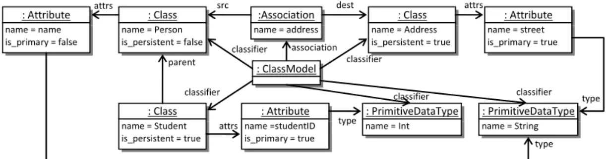
The class diagram example is represented in Figure 1(a) using a graphical syntax close to UML. In MDE, this model could be represented with an abstract syntax where each element is defined
as an instance of a metamodel class. This level of detail is close to the way model transformation manipulates a model and will be useful in the proposed contributions. In Figure 3, the class diagram of Figure 1(a) is represented with this abstract syntax.
: Class name = Student is_persistent = true : Class name = Person is_persistent = false : Class name = Address is_persistent = true :Association name = address : Attribute name =studentID is_primary = true : Attribute name = street is_primary = true : Attribute name = name is_primary = false : PrimitiveDataType name = String : ClassModel : PrimitiveDataType name = Int attrs attrs attrs association parent classifier classifier type type classifier classifier type classifier
src dest
Figure 3. The Input Model Example as an Instance Diagram of the Input Metamodel of class2rdbms
2.3. Model Transformation
Model transformationsallow the automatic production or modification of models and present thus a major interest for MDE [14]. A model transformation is based on its input and output metamodels specifying respectively its input and output domains. Basically, the transformation establishes a set of relationships between input model elements and output model elements.
class2rdbms transforms an input simple class diagram model into an output RDBMS model. Such a simple class diagram model is illustrated in Figure 1(a). A person has a name and an address, and she could be a student with a studentID. class2rdbms transforms this model into the RDBMS model of the Figure 1(b). Briefly, the persistent classes are changed into tables. The attributes and associations become columns. Primary attributes (underlined) become primary keys PK and the associations become foreign keys FK. Figure 2(b) presents the RDBMS metamodel, defining the output model elements.
Concretely, a model transformation is expressed in a model transformation language. In order to describe a model transformation, many approaches and languages can be used. A classification of these approaches is proposed by Czarnecki et al. [15]. Most of the model transformation languages decompose transformation into smaller parts called rule such as a program is decomposed into functions. Practically, a rule focuses on the transformation of a specific input element. In this paper, the rule concept is used to express the way input elements are transformed. Moreover, even if the transformation approaches are different, they usually work in the same way. Indeed, most transformations aim to create a new model†, and can be considered as a set of three kinds
of operations: navigations between model elements in order to reach some specific elements;
f iltering of model element collections in order to express some conditions and keep only some
subparts of the initial collections; andcreations/modif icationsof new model elements. Listing 1 is an extract of the class2rdbms transformation written in QVTo [16]. Examples of navigation can be found all over the listing and are expressed using dot notation. Line 5 and the expression between brackets line 10 illustrate filtering. Creations are expressed with the mapping of object key words. In other languages like Kermeta (see Listing 2, page 23), these operations are differently specified.
Listing 1: Extract of the class2rdbms transformation in QVTo
1 transformation class2rdbms (in srcModel:UML,out dest:RDBMS);
2 [...]
3 -- maps a class to a table, with a column
4 mapping Class::class2table () : Table
5 when {self.kind=’persistent’;}
6 {
7 name := ’t_’ + self.name;
8 column := self.attrs->map attr2OrdinaryColumn();
9 key_ := object Key { -- nested population section for a ’Key’
10 name := ’k_’+self.name; column := result.column[kind=’primary’]; };
11 }
12 -- Mapping that creates an ordinary column from a leaf attribute
13 mapping Attribute::attr2OrdinaryColumn (): Column {
14 name := prefix+self.name;
15 kind := self.kind;
16 type := if self.attr.type.name=’int’ then ’NUMBER’ else ’VARCHAR’ endif;
17 }
2.4. Model Transformation Testing
Obviously, model transformation may be considered as a program and consequently tested. However, existing approaches do not take into account the specific features of model transformations, i.e. (i) the three fundamental operations composing them and (ii) models as input data. Traditional testing approaches have thus to be adapted to model transformations. Such adaptations may be performed for each specific transformation language / approach or in the opposite may take into account their heterogeneity. The approach proposed in this paper adopts the second alternative relying on the common features of the transformations.
As seen before, the definition of model transformations relies on their input and output metamodels. Thus to test the transformations, the elements of the input and the output models have to be considered as instances of the metamodel elements leading to large and complex graphs. Figure 3 illustrates the complexity of an input model example, despite the simplicity of that Class diagram model represented in Figure 1(a). Consequently, the generation and the evaluation of the test data, which are test input models, are complex. Moreover, this complexity increases by considering that the test data set (i) should cover the input domain of the model transformation, which may be very large, and (ii) should be able to detect faults in transformation. In addition, MDE development environments lack reliable support to analyze and transform models. Therefore, it is more efficient to propose techniques to automate or assist in the generation of test models, rather than to evaluate the efficiency of a test model set and leave the tester to manage to improve it manually.
In this paper contrary as in other works [17, 18], the test oracle challenge is not concerned.
3. IMPROVING A TEST DATA SET: STATE OF THE ART
Among the various proposed approaches, test model qualification provides information useful to generate efficient test data. Few works study test model qualification and generation, considering efficiency in terms of input domain coverage, model transformation rules coverage, specification coverage and potential fault coverage. First these different ways to obtain qualified test model sets are presented, then the focus is put on the last one with mutation analysis.
3.1. Test Model Qualification and Generation Approaches
Model transformation domains are specified with metamodel and several works consider that characteristic to qualify test model sets.
Fleurey et al. [19] qualify a set of test models regarding its coverage of the input domain. This approach is based on the partitioning of the metamodels. Sen et al. [20] developed the Pramana tool (formerly named Cartier) to generate test models based on the proposal of Fleurey et al. However, both approaches produce more models than necessary because they aim to provide tests covering the whole input domain, even if only a subpart of the input domain is used by the transformation. In the case of UML, it often occurs that transformations only deal with a subpart (e.g. the class diagram or the state diagram). To avoid producing test models relative to metamodel parts not involved in
the transformation, Sen et al. [21] prune the metamodel to extract only the subparts involved in the transformation before providing the tests.
Mottu et al. [22] propose a white-box approach that uses a static analysis to automatically generate test inputs for transformations. This static analysis uncovers knowledge about how the input model elements are accessed by transformation rules. On the other hand, because these approaches rely on static analysis of the transformation, if there is some dead code, tests are generated for these parts, even if they are never executed.
Guerra [23] tackles the test model generation challenge by deriving, from the transformation specification, a set of test models ensuring a certain level of coverage of the properties in the specification. These input models are calculated using constraint solving techniques.
Those approaches study transformations only statically, i.e. without executing them and without considering the potential errors. As a result, a 100% mutation score has not yet been reached in the experiments of those papers (70% [23], 89.9% avg. [20], 97.62% avg. [22]). Moreover, these methods help to generate qualified test models without providing information and methods to improve test models when highest quality is mandatory (for example, in case of the generation of highly critical applications). In the opposite, the contributions proposed in this paper help the tester to improve the quality of test models set thanks to mutation analysis enhanced with mutation operator metamodeling and traceability.
3.2. Mutation Testing Approaches to Measure Test Data Set Efficiency to Detect Faults
Numerous papers study mutation testing in a general context. Jia et al. propose a survey on mutation testing development [24]. They observe an increase of mutation testing publications from
1978(mutation testing emergence) to 2009making the mutation testing a mature technique. The main problem tackled in the literature is the creation of mutation operators. In this subsection, works related to the design of mutation operators are discussed and, in the next subsection, the improvement of the test data quality with mutation testing.
Several works advise to use mutation testing [25, 26, 27]. They analyse its ability to qualify test set with a high fault power detection and with different properties (for instance, test sets with fewer test cases). Those papers compare mutation testing with edge-Pair [28], All-uses [29] and Prime Path Coverage criteria (line coverage or statement coverage) [30] techniques, concluding that mutation testing provides better results.
Most of the works consider the mutation operators directly based on the syntax of a programming language: C [31], ADA [32], Java [33]. These mutation operator sets take into consideration the programming paradigm of the language (e.g. procedural [34], object oriented [33]). However, they are defined using the syntax of a programming language.
To fit with model paradigm and model transformations, Mottu et al. proposed an adaptation of mutation testing [9]. The originality of that work was not to use a programming syntax to define mutation operators, but to consider abstract operations applied by the transformation on models. Based on this work, Tisi et al. propose to formalize these mutation operators as a set of higher-order transformations (HOT) (i.e. transformations whose input or output model is itself a transformation [35]). For instance, Fraternali et al. propose an implementation of Mottu
et al. operators as ATL HOTs [36] (ATL is a specific model transformation language). Some transformation languages do not use a model as an internal representation of the transformations. The approach proposed by Tisi et al. [35] can thus only be used for transformation languages supporting such a representation.
Few works consider mutation operators independently from the syntax of a language. Mutation operators proposed by Ferrari et al. are designed considering aspect oriented programming characteristics [37]. Recently, Sim˜ao et al. [38] proposes MuDeL, a language used to precisely define mutation operators independently from the used language. They provide generic definitions of each operator that may be reused with several languages. They also use a compilation from MuDeL operators to the language syntax. However, the proposed generic definitions of operators do not consider the specificity of new programming paradigms (as model transformation in model-driven engineering) and new kinds of analysis and transformation of specific data (as models). Moreover,
MuDeL deals with context-free mutations (whenx = 2becomesx+ = 3it is context free but not when it becomesy = 2) whereas in the approach proposed in this paper, several mutation operators are not context free (for instance, some operators require to know the elements of the metamodel to perform the mutation of the transformation rules).
3.3. Mutation Analysis to Improve Test Data
Several works deal with test set improvement to increase mutation score. Fleurey et al. propose an adaptation of a bacteriologic algorithm to model transformation testing [39]. The bacteriologic algorithm [40] is designed to automatically improve the quality of a test data set. It measures the power of each data to highlight errors to(1)reject useless test data,(2)keep the best test data,(3)
combine the latter to create new test data. Their adaptation consists of creating new test models by covering part of the input domain still not covered.
MuTest is a project that aims to use mutation analysis to drive test case generation [41]. In order to produce new test data, MuTest generates multiples assertions to kill a selected mutant. Once the new test data is found, the test set is minimized in order to keep the test set as small as possible.
EvoSuite is a tool which is able to improve automatically a test set for the Java language [42]. It relies on mutation testing to produce a reduced set of assertions that maximizes the mutation score. In order to produce the new test data, EvoSuite tries to find test cases that violate the oracles. However, this tool directly handles Java byte code, and it is so close to the Java language that it makes its adaptation particularly difficult.
Some other works use evolutionary and genetic algorithms for automatic test input data generation in the context of mutation testing. A fully automated ant colony optimization algorithm is provided by Ayari et al. [43]. From an initial test set, the algorithm progressively promotes best test cases and combines them to generate new test data in order to kill mutants. The authors obtain a maximum mutation score of89%on a small Java program.
However, all of these works only consider traditional programming, even if some propose bacteriologic algorithm for component based programming [39]. They do not take into account the particularities of model transformations (such as models as input data) ,and prevent their use for model transformations, as explained in the introduction.
4. MUTATION ANALYSIS AND MODEL TRANSFORMATIONS
Mutation analysis relies on the following assumption: if a test data set can reveal the faults voluntary and systematically injected in various versions of the program under test, then this set is able to detect involuntary faults. The efficiency of the test data set to detect the injected faults is evaluated by calculating the mutation score, i.e. the proportion of detected faulty versions [3]. Next subsections present the mutation analysis process adapted to model transformations and the challenges considered in this paper.
4.1. Mutation Analysis Dedicated to Model Transformations
Model transformations have their own specificities such as the manipulated data structures (i.e. models which conform to their metamodels) or characteristic operations that may lead to semantic faults. The mutation analysis process for traditional programs [44] has been adapted to model transformations [9]. It is presented in Figure 4. The four main activities are the following.
Preliminary step (activity(a)): this activity is divided into two parts: the creation of mutants and an initial test data set creation. Mutants are defined by modifying an instruction in a transformation rule from the original model transformation. This rule which owns the modified instruction is called mutated rule in the remainder of the paper. The modification of the instruction is performed using one of the mutation operators dedicated to model transformations [9]. These operators have been defined independently from any transformation language. They are based on the three basic operations performed by a model
Legend Activity Data
Repeated Activity Sequence Between Activities
Data Consumption Data Production Preliminary Step Operators Execution [too weak] Models Mutation Score Computation Test Set Improvement
Figure 4. Mutation Testing Process Dedicated to Models
transformation: the navigation through references between objects in models, filtering of objects collections and the creation (or the modification) of model elements. An initial test data set containing several test models is possibly automatically built, using approaches such as the ones discussed in section 3.1.
The mutant and original program execution (activity(b)): each created mutantT1,T2, . . . , Tk,
as well as the original non-mutated transformationT is executed on each input test model. The mutation score computation (activity(c)): the mutation score is the proportion of killed
mutants compared to the overall number of mutants. A mutant is marked as killed when one (or several) test model highlights the injected error. A test model highlights an error if the result of its execution by the mutant differs from the execution by the original transformation. Thus, if for a given test modelm,Ti(m) 6= T (m)thenTi is killedelseTi isalive. Output
model comparison can be performed using adequate tools adapted to models or large graphs such as EMFCompare [45]. The mutation score computation is thus automatically performed. The test data set improvement (activity(d)): if the mutation score is considered too low, new test models are produced in order to kill live mutants; and equivalent mutants are rejected [24] (these last have the same behaviour than the transformation, so they are not considered being faulty).
Although, once again as the classical mutation testing process, the whole process starts again until the mutation score reaches a beforehand fixed threshold,100%is ideal [4].
4.2. A Process Remaining Mainly Manual
Although some tasks of the mutation testing process are automatic, this process remains a complex and long work for the tester. For any program under test (including model transformation), among the mutation testing tasks:
• creation of mutantscan be automated. However, mutation operators are applied to the code of the program under test. Thus, for each new language, mutation operators must be designed in its syntax (or ported from non syntactic ones [36]), and implemented,
• executionof the program and the mutants is an automated task,
• comparison of the output datais also an automated task.
The test data set improvement task (requiring analysis of mutants), is considered as time-consuming [26] and is currently performed manually. Indeed, injected faults which are not highlighted by test data must be analysed in both ways: statically (i.e. using a static analysis of the code) and dynamically (i.e. an execution of the program is required) in order to create new data which could kill a live mutant. The result of activity (a) is considered in the remainder of the paper as a prerequisite.
This paper focuses on the test data set improvement task (activity(d)) for the mutation analysis process dedicated to model transformations.
4.3. Contribution to Model Transformation Mutation Analysis
This paper proposal is based on the following hypothesis: building a new test model from scratch can be extremely complex, while taking advantage of existing test models could help to construct new ones. Consequently, an approach helping to create new test models from modifications of relevant existing models has been developed. Thus, first, a relevant test model is selected to be modified. As the work deals with a large amount of information, the induced problems could be resumed in three questions:
• Among all the existing pairs(test model, mutant), which ones are the most relevant to be studied? Moreover, in those models, which parts are relevant to improve the models?
• Why a mutant has not been killed by a specific test model?
• How to modify a selected test model to produce a different output model and thus kill the studied mutant?
In this paper, answers to these three questions are provided and thus the automation of the test data set improvement activity of the mutation analysis process is improved. The approach is composed of two major steps: (i) the selection of a relevant pair(test model, mutant)and (ii) the creation of a new test model by adequately modifying the one identified. The first step relies on an intensive use of the model transformation traceability [46]. It is briefly reminded in Section 5. The second step corresponding to the heart of this contribution is presented in Section 6 and 7. Both steps are illustrated in Section 8, and are experimented in Section 8.9.
5. MODEL TRANSFORMATION TRACEABILITY: A WAY TO COLLECT INFORMATION This Section reminds previous works [46] proposing a systematic procedure to answer the first question: “Among all the existing pairs (test model, mutant), which ones are the most relevant to
be studied? And in those models, which parts are relevant to improve the model?” The principles of model transformation traceability are summarized, the mutation matrix is introduced and the relationships between these two concepts are detailed.
5.1. Model Transformation Traceability
Regarding MDE and more specifically model transformations, the traceability mechanism links input and output models elements [47]. It specifies input model elements used by the transformation to generate output model elements.
Excerpt of Input Model Sample
: Class
name=Person
is_persistent =false : Class
name=Address is_persistent =true parent src dest attrs : Column name= type=String Link1 : Class name= is_persistent =trueStudent
Link2 : Table name=Student :Association name=address : Attribute name=
is_primary=truestreet address_street
cols
Excerpt of Output Model Sample Model transformation
transform createColumns
Excerpt of Trace Link3
Figure 5. Trace Example
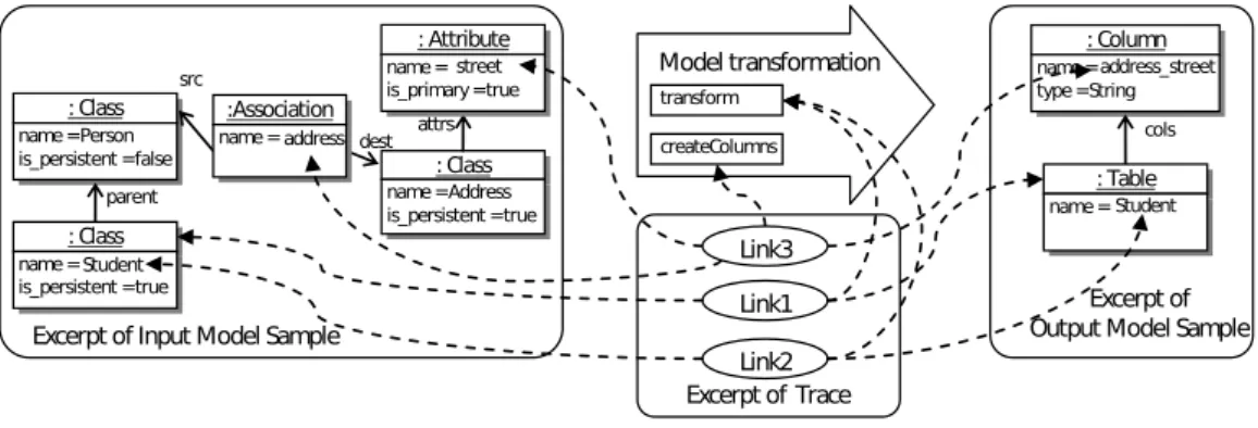
Various traceability approaches have been developed, but they are dedicated to a specific transformation language [48], [49], [50] or they take into account only classes and not attributes [47]. A traceability approach has been developed [51] independently from any transformation language. Each creation/modification of an element by a rule leads to the creation of a unique link. Each
link refers to (i) a set of source elements (attribute or class instances), (ii) a set of target elements and (iii) the transformation rule that leads to this creation/modification. Each link corresponds to an execution of a rule, that may be executed several times on different input elements. Figure 5 illustrates an example.Link1indicates that the output instance ofT ablehas been created from one input instance ofClass. Moreover,Link1specifies that the instances it binds have been read and created by thetransf ormrule.
Each trace is formally modeled. It captures formal relations between models and the transformation. Moreover, it can be analyzed independently from any transformation language. Nevertheless, the automatic generation of traces must be tied to a specific transformation language. In this paper, the trace generation is adapted for the Kermeta‡ language in order to pursue the
works initiated by Mottu et al. [9, 20]. Usually traces can be automatically generated without altering the transformation by adding plugins to the transformation engine [51]. However, these solutions rely on an intermediary internal representation of the transformations used by other transformation languages such as QVTo [16]. Kermeta does not use any intermediary representation. Two alternatives remain: drastically modifying the engine or manually inserting instructions in the transformation [48]. This latter solution has been adopted in the experimentations since it allows quick prototyping and requires a small development effort§.
5.2. Model Transformation Traces and Mutation Matrix Generation
The execution step named(b)in Figure 4 is more complex than just executing the mutants for each test model. A trace model is generated for each execution and a mutation matrix [9] is built to gather all the results. Figure 6 sketches this step that has been detailed in [46].
Mutant Execution Mutation Matrix Trace Models [Test Model?] Status Definition Transformation T Execution Original TransformationT Execution
Figure 6. Mutation Matrix and Trace Generation
The execution step requires the following parameters: the transformation under testT, its mutants
Tiand the test models. For each transformation execution (original or mutant), a trace (Trace Model)
is produced and associated to the corresponding pair(test model, mutant). Furthermore, the state (i.e. killed or alive) for this pair is stored in a cell of the mutation matrix.
More precisely, each cell of the mutation matrix corresponds to the execution of a mutantTiwith
a test modelmj. The mutation matrix is presented in Figure 7. It is organized through three main
concepts [46]:
• Mutant(T0. . . Tn) which represents the executions of a mutant in a column,
• Model(m0. . . mm) which represents the transformations of a test modelmjin a row,
• Cell(C00. . . Cmn) which represents the execution of one mutant with one single test model.
It specifies if the test model lets the mutant alive or not (with aboolean). Furthermore, each cell is associated to a Trace (lt00. . . ltmn).
Thus, from a Mutant or a Model, it is possible to access to its Cells and so to its Traces. The mutation matrix acts as a pivot between the mutants, the test models and the traces. It is then used
‡http://www.kermeta.org §Experimental material [52]
Mutants M od el s T T1 ... Tn m0 m1 mm c00 c01 ... c0n c10 c11 ... c1n cm0 cm1 ... cmn ... ... ... ... ... lt00 lt01 ... lt0n lt10 lt11 ... lt1n ltm0 ltm1 ... ltmn ... ... ... ... Traces
Figure 7. Mutation Matrix
to define final status of the mutant. Indeed, if a mutant has no cell marked as killed, it is considered as alive.
5.3. Identification of Relevant Pairs (Model, Mutant)
The proposed approach relies on the assumption that test models owning elements which are used by the mutated rule (and so by the mutated instruction) are good candidates to be improved to kill the mutant. Indeed, this rule has been executed on elements of these test models, but the resulting models do not differ from the ones of the original transformation executions possibly because of neutralization by the remainder of the transformation. The mutant is the exact copy of the original transformation except the mutated instruction. The difference of the outputs can only result from the execution of this mutated instruction and thus of the mutated rule. The traceability mechanism allows the tester to identify these candidate models and, for each one, to highlight the elements consumed and produced by the mutated rule. Thus, the test model improvement activity (Figure 4, activity(d)) is decomposed into three steps as illustrated in Figure 8.
Operator Test Model Trace Model
Test Model Set Improvement Mutation Matrix Live Mutant Selection Relevant Test Model Identification New Test Model Creation Test Model
Figure 8. Test Model Set Improvement Process
Live Mutant Selection. The selection of a relevant pair begins by the choice of a live mutant (activity(1)). This is automatically performed by exploring the boolean attribute of the mutation matrix cells.
Relevant Test Model Identification. For the selected mutant, the corresponding cells of the mutation matrix are explored, and each trace model is navigated to identify if the mutated rule has been executed, i.e. if, in the trace, there exists alinkpointing to it. Two situations can occur: (i) If the rule has never been executed, a new test model must be created, potentially from scratch, taking care that conditions for the mutated rule to be executed are fulfilled. (ii) If the mutated rule has been called at least once the algorithm selects some candidate test models. Moreover, for each identified test model, two other sets are provided representing respectively the input and the output elements handled by the mutated rule. Among these models, the one with the smallest sets of elements is selected: using the two sets associated to the chosen model, the tester can focus on the smallest set of input model elements and its small counterpart in the output model to understand why these elements do not kill the mutant being considered and consequently to modify the identified model. Using the input model with the smallest set of elements reduces the space search and, consequently, the effort to analyse why its elements do not kill the mutant.
3 3a
3b
3c
New Test Model Creation
Mutation Matrix
Trace Model Operator Test Model Test Model Handled
Parts Identification ModificationTest Model Initial Test
Model Copy
Figure 9. New Test Model Creation Process
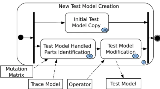
New Test Model Creation. In order to increase the test model set without regression (i.e. without making alive some mutants killed by the identified test model), this identified test model is preliminary copied as shown in Figure 9, activity 3(b) and then modified. The activity2 has provided the input and output elements handled by the mutated rule. According to the mutant and the applied operators, the input or the output elements are identified in the corresponding model (Figure 9, activity 3(a)). Section 7 focuses on the modification of the test model (activity 3(c)) to automate and assist this activity which is manual until now. The mutation matrix and the trace may be used to automatically identify relevant pairs(test model, mutant)and the input and output elements involved in the execution of the mutated rule. In the next section, the mutation operators automatically use them as input of the3(c)activity (Figure 9).
6. MODELLING MUTATION OPERATORS
In order to automate the treatment of the live mutants, mutation made in them should be more precise than an informal description (as it was proposed by Mottu et al. [9]). The mutation operators are designed to automatically detect where they could be applied. The heterogeneity of model transformation languages issue is prevented by using a language independent approach. Moreover, only the modification and creation of new test models that are not dependent on the transformation language are addressed.
The original contribution consists in modeling mutation operators based on their effects upon the data manipulated by the transformation under test instead of based on their implementation in the transformation language being used. The mutation operators proposed by Mottu et al. [9] are thus designed based on the metamodels of the models manipulated by the transformation.
6.1. Principle
The mutation operators for model transformation are based on the three classical operations that occur in model transformations: navigation, filtering, and creation (or modification) of input and output model elements [9]. These three operations are sequentially applied. They form a basic cycle which is repeated to compose a whole model transformation. Such a decomposition into elementary operations provides an abstract view which is useful for fault injection.
Each mutation operator is designed as a metamodel expressing how the operator may be applied on any transformation. The 10 mutation operators defined by Mottu et al. [9] lead to the creation of 10 mutation operator metamodels. Those metamodels are independent from any transformation and any transformation language. Their instantiations depend on the transformation under test and express how mutants operate on its input/output metamodels. A single instance can be used to represent a kind of mutation applied to several code areas leading to the creation of several mutants. The application of one mutation operator on one transformation returns mutation models which conform to the corresponding mutation operator metamodel. Whereas a mutation metamodel is generic, its models are dedicated to one model transformation, but still language independent.
Class is_persistent : Boolean Association name : String Attribute name : String is_primary : Boolean PrimitiveDataType ClassModel attrs association parent type classifier src dest Classifier name : String 1 1 * * 1 1..* 0..1
(a) Simple Class Diagram Metamodel
eAttributes Eclass EAttribute EDataType EReference eReferences eReferenceType eSuperTypes eOpposite eAttributeType 1 0..* 0..* 0..1 1 0..* EMOF MM (b) EMOF Meta-Metamodel
Figure 10. Class diagram metamodel and its own metamodel: EMOF meta-metamodel
Those mutation models are based on the input and output metamodels of the transformation. They define how input/output model elements could be treated by the original transformation and how the mutants would treat them. For instance, Figure 10(a) reminds the metamodel of the class2rdbms transformation. One mutation model would describe that the srclink is navigated instead of the dest link. Another mutation model would describe that the destlink is navigated instead of the src link. Another one would select a subset of Class instances in a set collected through theclassif ierlink.
The application of one mutation operator model on one transformation implementation returns the mutants. This step is out of the scope of this paper since it depends on the transformation language. To understand how those mutation operator metamodels are created and then instantiated in mutation operator models, the concept of metamodel needs to be further explained.
A metamodel is itself a model, and thus it conforms to one metamodel which defines its concepts. This metamodel called meta-metamodel is the EMOF meta-metamodel and is illustrated in Figure 10(b). The class diagram metamodel (Figure 10(a)) conforms to the EMOF meta-metamodel. Thus, for example, Class and P rimitiveDataT ype are instances of EClass whose eSuperT ype is
Classif ier, another instance of EClass. is persistent, is primary, or name are instances of
EAttributeand theirEDatatypeareBoolean,Boolean, andString, respectively.destandsrc
areERef erencewithouteOpposite ERef erence.
6.2. Three Examples of Mutation Operator Models
The following subsections present the metamodels of three mutation operators with definition extracted from Mottu et al. work [9], an application example extracted from the class2rdbms transformation, and a description of the used concepts and relations. For the sake of conciseness, the 7 other mutation operators are detailed in an annex [52]. In order to create the mutants, the effective operators applied to the transformation under test (i.e. the mutation operator models) have to be effectively defined. This is automatically performed with a model transformation [52].
6.2.1. Navigation Mutation: Relation to the Same Class Change Operator (RSCC)
Definition “The RSCC operator replaces the navigation of one reference towards a class with the navigation of another reference to the same class.”
The RSCC operator can be applied on the input or the output metamodel of the transformation but only if it exists, in the metamodel, at least two EReferences between the two same EClasses. One EReference is originally navigated, the other is navigated by a mutant. Thus applied on a model transformation, RSCC operator replaces the original navigation by another to the same EClass.
The RSCC operator metamodel is presented in Figure 11. In order to ensure its independence from any transformation and transformation language, it is expressed on generic concepts that can appear in any transformation whatever the used language. Indeed, the RSCC operator metamodel uses the EMOF metamodel (on the left of Figure 11) to specify the input or output elements of the transformation the operator is applied on. Note that for each operator metamodel, several abstract
classes have been introduced (on the right) refactoring some references and increasing reusability between operator metamodels as shown in the Annex [52].
eAttributes Eclass EAttribute EDataType EReference eReferences eReferenceType eSuperTypes eOpposite eAttributeType 1 0..* 0..* 0..1 1 0..* Navigation Replacement RSCC newNavigation 1 initNavigation 1 EMOF MM
Figure 11. RSCC operator metamodel
Metamodel Description Table I gathers the classes and the relations dedicated to the RSCC operator. Additional constraints are necessary to ensure the viability of the mutant created. The first constraint prevents the mutants to be equivalent. The second constraint requires the two EReferences being to the same EClass.
CLASS/RELATION DESCRIPTION
RSCC The mutation operator
initNavigation EReference initially navigated by the transformation
newNavigation EReference navigated after the mutation
additional constraint newNavigation != initNavigation
additional constraint newNavigation.eReferenceType = initNavigation.eReferenceType
Table I. Description of the RSCC Operator Metamodel
Example The mutation model illustrated in Figure 12 is an example of the application of the RSCC mutation operator on the class2rdbms transformation. The grey part instantiates the operator RSCC. This mutation model would be applied in the transformation each time a rule navigates the dest EReference (replacing it with the src EReference), whatever its place in a navigation chain, returning each time a different mutant. Note that the RSCC operator metamodel would be instantiated a second time by invertinginitN avigationandnewN avigation.
Class is_persistent : Boolean Association name : String Attribute name : String is_primary : Boolean PrimitiveDataType ClassModel attrs association parent type classifier src dest Classifier name : String 1 1 * * 1 * 0..1 Op1 : RSCC initNavigation newNavigation
Figure 12. One example of the RSCC mutation models for the class2rdbms transformation
Such a mutation operator model could then be applied to the implementation of the transformation. For instance, the following mutant has been produced in the Listing 3, page 23, written in Kermeta with its mutated navigation Line 3.
6.2.2. Filtering Mutation: Collection Filtering Change with Addition (CFCA)
The filtering operations handle collections and select a subset of elements useful for the transformation; based on specific criteria. The collection may be collected by an eAttribute or through an EReference, or it may be an EClass collection.
Definition “This operator [. . . ] uses a collection and processes [an extra] filtering on it. This operator could return an infinite number of mutants and need to be restricted. It has been chosen to take a collection and to return a single element arbitrarily chosen.”
Figure 13 and Table II describe the metamodel of the CFCA mutation operator.
eAttributes Eclass EAttribute EDataType EReference eReferences eReferenceType eSuperTypes eOpposite eAttributeType 1 0..* 0..* 0..1 1 0..* Filter CardFilter CFCA attributeFrom eRefFrom 0..1 dataTypeRes 0..1 eClassRes 0..1 EMOF MM 0..1 eClassFrom 0..1
Figure 13. CFCA operator metamodel
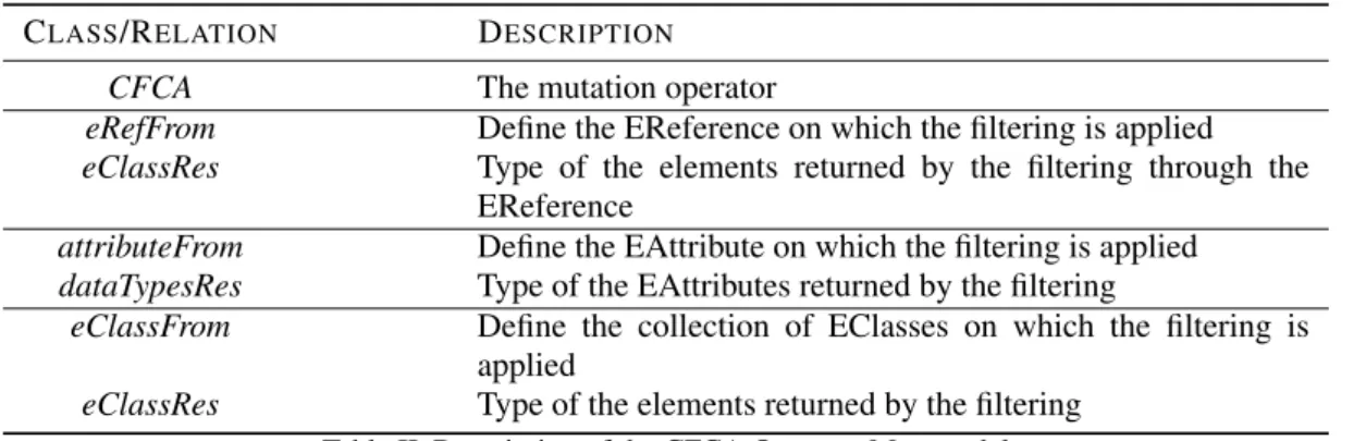
Metamodel Description Table II gathers the classes and the relations dedicated to the CFCA operator. The table is divided into several parts because the three last ones are mutually exclusive. In fact, the filter may concern either an EReference, an EAttribute (both pointing collections of element), or a collection of EClasses and that also appears in the cardinalities associated to the
eRef F rom,attributeF rom, andeClassF romEReferences. The fault is not directly described in
this metamodel (as it was withnewN avigationin RSCC), since the operator modifies the original filter, arbitrarily, selecting only one element, for instance.
CLASS/RELATION DESCRIPTION
CFCA The mutation operator
eRefFrom Define the EReference on which the filtering is applied
eClassRes Type of the elements returned by the filtering through the EReference
attributeFrom Define the EAttribute on which the filtering is applied
dataTypesRes Type of the EAttributes returned by the filtering
eClassFrom Define the collection of EClasses on which the filtering is applied
eClassRes Type of the elements returned by the filtering
Table II. Description of the CFCA Operator Metamodel
Example Figure 14 illustrates one mutation model of CFCA applied to class2rdbms transforma-tion. The grey part instantiates the operator CFCA whereas the remainder is the input metamodel of the transformation. This mutation model would be applied to the transformation each time a rule filters a collection of Classinstances returned by theclassif ier reference. i.e. if aClassM odel
has severalClasses(such as in Figure 1a), CFCA operator modifies the filter to select only one of
theClassin the model.
6.2.3. Creation Mutation: Classes’ Association Creation Addition (CACA) Operator
The creation mutation operators are relative to the last phase of the transformation process (i.e. they concern the creation or modification of output metamodel elements).
Definition “This operator adds an extra relation between two class instances of the output model, when the metamodel allows it.”
Class is_persistent : Boolean Association name : String Attribute name : String is_primary : Boolean PrimitiveDataType ClassModel attrs association parent type classifier src dest Classifier name : String 1 1 * * 1 * 0..1 Op2 : CFCA eRefFrom eClassRef
Figure 14. One example of the CFCA mutation models for class2rdbms transformation
The creation operators (e.g. CACA) are defined on the output metamodel of the transformation. The output model resulting from the execution of the original transformation or from a mutant must always conform the output metamodel. Thus, the mutant may add in the output model only references that are instances ofERef erencesin the output metamodel. Moreover, according to [9], if the EReference has an upper cardinality equals to 1 and if an instance already exists, then adding an extra has no consequence, the EReference is overridden. The CACA operator metamodel is illustrated in Figure 15. eAttributes Eclass EAttribute EDataType EReference eReferences eReferenceType eSuperTypes eOpposite eAttributeType 1 0..* 0..* 0..1 1 0..* Creation Modification CACA refToModify 1 EMOF MM
Figure 15. CACA Operator Metamodel
Metamodel Description Table III sums up the description of the CACA metamodel by describing its specific classes and relation. For this mutation operator, the refToModify EReference corresponds to the reference which is added in the output model.
CLASS/RELATION DESCRIPTION
CACA The mutation operator
refToModify EReference added by the mutant
Table III. Description of the CACA Operator Metamodel
Example Figure 16 illustrates one mutation model of CACA applied to class2rdbms transfor-mation. An EReference references from aF Keyinstance to aT ableinstance is wrongly added in an output model. Since the ref erencesEReference has a cardinality of1 and may have already been initialized, the EReference is simply overridden.
The other operators are described using the same technique in the Annex [52]. In order to use these models, it is necessary to bind them with the other models corresponding to the tested transformation or the mutants, the trace and the test models. The mutation matrix already plays a pivot role between these latter; it is thus modified to also handle the mutation models.
cc
CACA refToModifyFigure 16. CACA Operator Application Example
6.3. Mutation Matrix Binding
Each mutant is returned by a single application of one mutation operator on the original transformation. In order to enable a direct access from a given mutantTjto its associated operator
Opk, a link is added to each mutant in the mutation matrix, as shown in Figure 17. Two mutantsT0
andT1may be linked to the same mutation operator model. Indeed, as an instruction can be used
many times at different places in a model transformation (as in traditional programming), a same mutation operator modelOpkcan fit for several mutants.
Op1 Op2 Opk Mutation Operator Models ... c c c c c c c c c
Figure 17. Mutation Matrix and Mutation Operator
7. CREATION OF A NEW TEST MODEL BY MODIFYING AN EXISTING ONE BASED ON PATTERN IDENTIFICATION
Based on the abstract representations of the operators and their definition on the input or output metamodel of the transformation, it is possible to identify why a mutant remains alive, and give some recommendations to modify existing test models that in their new versions should kill the mutant. For each mutation operator, few test model patterns (i.e. specific configurations in the model) leaving a mutant alive are identified. For each pattern, modifications that should kill the mutant are identified. This solves the two unresolved issues: “Why a mutant has not been killed by
a specific test model?” and “How a selected test model could be modified to produce the expected
output model and thus kill the studied mutant?”. It has to be noticed that the following works are specified at a meta level based only on the abstract representation of the operators. It is not possible to be absolutely sure that the recommended modifications applied to a test model will kill the mutant. In other terms, the approach proposed in this paper provides an automatic analysis of the situation and advises some first modifications to be performed; in a lot of cases, they will be enough to kill the mutant.
7.1. Presentation of the Patterns Notion on the RSCC operator
In this subsection, some cases (also called patterns) that may let a mutant alive are illustrated. For example, the RSCC- Relation to the Same Class Change operator is considered. This operator replaces the navigation of one reference towards a class with the navigation of another reference to the same class (cf. 6.2.1). Thus, for an original transformation navigating theself.a.ba.csequence, one mutant may navigate the self.a.bb.csequence. The dot notation is used as in object oriented languages to navigate from one class to another:selfrefers to a class,a,baandbbto references, and
ceither to another reference or an attribute (see Figure 18 for an example of possible input models for this transformation). For this operator, three patterns letting the mutant alive are identified:
• Pattern 1: the original sequence and the mutated one finally point to the same instance,
• Pattern 2: the original sequence and the mutated one finally point to null,
• Pattern 3: the value of the element property pointed by the original sequence and the mutated one are the same.
These three patterns are represented in Figure 18 on three simple models and described below. Those models would have been selected because they execute the mutated rule without killing the mutant (following the process of the Section 5). The way to modify the test model is different according to the pattern.
b1: B a c2: C label = "tmpLab" s1: S a a1: A Pattern 1 example Pattern 3 example Pattern 2 example label = "tmpLab" b2: B ba bb s1: S a1: A c1: C b1: B a label = "tmpLab" b2: B ba bb s1: S a1: A c1: C c c c c
Figure 18. Patterns Examples
Pattern 1 The first pattern occurs when either the mutated navigation points to the same element as the original navigation (baandbbpoint to the same instance ofB) (not represented in the Figure) or the original sequence and the mutated one point to the same instance (as in the Figure).
The mutant can be killed if the mutated and the original navigation sequences point to two different instances of the same EClass. To produce the new test model, a new instance of this EClass, with different attribute values, is added to the model and the EReferences are updated.
Recommendation for Pattern 1: the idea is to add a new instance completely different from the one recovered by navigating the original EReference. This recommendation, albeit simple, may not
killa live mutant. It may therefore be more appropriate to add an element in the collection handled by the mutant:
• If at least one of the two EReferences (original or mutated) has its upper bound strictly greater than1 (1 − nand 1 − ∗EReferences, i.e. collections), a new instance is added into the collection. Indeed, adding a new instance into a collection handled by the mutant or the original transformation can greatly influence the navigation results.
• If at least one of the two EReferences has its lower bound equal to0, it is possible to delete that instance. Thus, the original transformation or the mutant could not recover the instance and could return a different result (according to the deleted reference).
Pattern 2 The second pattern occurs when an intermediate reference cannot be navigated. In this example, if theareference (orcreference) points to null, neither the original sequenceself.a.ba.c
nor the mutated oneself.a.bb.ccan be fully navigated. The element recovered by the two sequences is null.
The selected test model can then be modified by updating empty references, i.e. by updating the
nullreference to an element with the correct type.
Recommendation for Pattern 2: once again, the idea is to add a new instance. As for the previous pattern, a new instance is created and the reference navigated by the original transformation is updated in order to point to this new object.
Pattern 3 The third pattern occurs when the elements recovered by the original sequence
self.a.ba.csequence and by the mutated oneself.a.bb.chave the same value for a given attribute
(e.g. an attribute named “label” with valuetmpLab).
To solve this problem, the tester can modify one of the attributes by changing its value.
Recommendation for Pattern 3: this time, it is the value of the properties that must be modified. Thus, once the elements handled by the faulty rule are identified, the value of their attributes is changed to create a new test model.
Automatic Pattern Detection: for each element retrieved by the algorithm described in Section 5.3 (elements handled by the mutated rule), references pointed by initNavigation and
newNavigationare navigated. These instances are then compared with each other in order to detect if they are the same (Pattern 1) or null(Pattern2). If the instances are different, their attributes are compared in order to detect common values (Pattern3). According to the identified pattern, the model can be modified.
7.2. Patterns for the CFCA Operator
The mutants created by the application of the CFCA operator select a single item in a collection. The mutant remains alive, because the original filter did not return any element or returned a single element. Indeed, if no item is returned by the original filter, the mutated filter will also return an empty set. Similarly, if one element is returned by the original filter, the mutation will have no effect. In both cases, the mutant and the original transformation will behave the same way. In the opposite, if the filtered collection contains several elements, a different behaviour should be highlighted between the original transformation and the mutant.
Without a complete specification of the filtering condition, it is difficult to provide a seamless solution to produce a new model. Nevertheless, it is possible to consider two patterns which let a mutant alive:
Pattern 1 the collection does not contain any element, Pattern 2 the collection contains only one element.
Automatic Pattern Detection: to automatically determine the number of items in the collection, the elements that are handled by the mutated rule and that are in the collection pointed by the eRefFrom EReference (respectively the collection of attributeFrom in case of collection of attributes) are selected (Figure 13). The number of items in the collection is then computed.
Recommendation for Pattern 1: if no element is present in the collection, two different instances satisfying the filtering condition are created and added to the collection. Adding only one element resolves the Pattern 1 but Pattern 2 would occur.
Recommendation for Pattern 2: if one element is present in the collection, an instance which satisfies the filtering condition is created and added to the filtered collection.
Depending on the complexity of the filtering condition, modifying an existing model can be tedious. In the cases not covered by the two proposed patterns, the recommendations will not be adapted; the s will have to study in details the input test models to create a new one. Nevertheless, the testers’ work is eased thanks to the traceability mechanism, by identifying the test model elements handled by the mutated rule.
7.3. Pattern for the CACA Operator
Creation operators inject faults that add, delete, or replace elements in the output models. Consequently, the probability to observe a difference between the mutated transformation output model and the original transformation output is higher than navigation or filtering operators. However, since the creation operators imply changes in the output model, patterns are not based on specific configuration in a test model.
The description of the operator [9] states that when the upper bound of the mutated EReference is 1, whatever the number of times an element is linked to others, only the last one is taken into account, all the previous ones are overridden. For EReferences whose upper bound is∗, the mutated instruction execution involves the addition of one extra element in the collection. So normally, the number of elements in the collection should be different in the output model resulting from the original transformation and the one generated by the mutant. If it is not the case, it may mean that this mutated instruction has not been executed.
Since the CACA operator concerns the output model, it is difficult to provide a seamless solution to produce a new model. Nevertheless, it is possible to consider three patterns which let a mutant alive. They are pretty vague since they are expressed directly on the output metamodel and not the input model. The associated recommendations are very generic; they concern the way to modify the input model.
Pattern 1 the cardinality of the mutated EReference in the output metamodel is0..1, Pattern 2 the cardinality of the mutated EReference in the output metamodel is1,
Pattern 3 the cardinality of the mutated EReference in the output metamodel is0..∗,1..∗orn..m
and this part of the rule has never been executed.
Automatic Pattern Detection: the model of the CACA operator applied to the mutant is automatically analysed in order to identify the cardinality of the output metamodel EReference pointed by the ref T oM odif y reference of the operator. The pattern3 is identified if the upper bound of the cardinality differs from 1 and if there is no instance of the EReference pointed by the
refToModifyreference in the output model.
Recommendation for Pattern 1: It is possible to apply an ad hoc modification; the idea here is to avoid the overriding of the original EReference. The output model element pointed by the original EReference must thus be removed. So, in the output model returned by the original transformation, the reference will point to no object, whereas the reference in the mutant output model returned by the mutated transformation should point to an element. To achieve that, the refToModify reference is navigated and the instance it points to is collected. The input model elements creating this instance are automatically identified using the trace. Finally, the choice of the input model elements to delete or modify is the only task left to the tester.
Recommendation for Pattern 2: As previously explained, only the last time the element is linked to others is taken into account. If a mutant whose CACA operator is applied to an EReference with cardinality 1 is alive, this means that the added reference and the original one lead to the same result. The way this element is obtained from the input elements has to be studied and consequently modified.
Recommendation for Pattern 3: The CACA operator adds an element in a collection. Since the mutant remains alive, this means that the part of the mutated rule has not been executed. The test model has to be modified in order to force the execution of this part of the mutant. Of course, it is possible that the mutation is applied to a dead code zone and in that case no test model will lead to its execution.
7.4. Synthesis
In this section, 8 patterns, 2 or 3 for each mutation operator have been identified. For the sake of conciseness, the patterns for the other mutation operators are explained in the Annex [52]. These patterns undoubtedly leave mutants alive. For each of these patterns, a modification of an existing input model has been proposed to create a new test model that should kill a mutant. However, for some operators, it may occur that the identified patterns are not enough and that a more detailed
Relevant Model and Elements Identification Model Creation Test Model
[is the mutated rule executed?] yes no Problematic Cases Detection Careful Mutation Analysis Modification Suggestion Model Modification Operator Test Model Trace Model
[is a case identified?] [is an automatic modification possible?] no yes yes no Trace Model Model Creation Test Model Manual Model Modification Test Model Automatic Task Semi-Automatic Task Manual Task
Figure 19. Choices During the New Test Model Creation
analysis is required. This analysis then relies on the results of the “relevant model and element identification” step (cf. 5.3).
To summarize the different steps of the proposed approach and their order, Figure 19 shows an activity diagram corresponding to the choices made by the final algorithm to support the creation of new test models. The process starts when relevant models and subparts of them are automatically identified. If the algorithm does not identify any relevant model, this means that the mutated rule has never been executed: this is the first information provided by the approach that helps testers. Therefore, the mutated rule must be analysed to determine the elements which are required to activate the rule execution, and a new test model is generated. If the mutated rule has been executed and if the mutant remains alive, the context must be analysed. The process then continues by trying to automatically identify whether the test model contains one of the proposed patterns. To perform this task, the modeled mutation operator and the model trace are used. When this activity is ended, if no pattern has been identified, the tester must semi-automatically analyse the mutant. To assist her in this task, the trace as well as the results of the “relevant model and element identification” step are provided. Once the mutant has been analysed, the tester can manually create the new test model. However, if a pattern has been identified, the proposed recommendation can be automatically implemented, a new test model is automatically created. For patterns where the change cannot be automatically performed, a modification suggestion is reported to the tester to help her to create a new test model.
Although the process is not fully-automated, assistance is provided thanks to the identification of relevant models and elements, the trace that helps to understand the transformation or the mutant execution, and the recommendations associated to the patterns.
8. CASE STUDY
In this section, the approach is deeply illustrated with the class2rdbms transformation. An initial test set is provided. In order to increase the mutation score, the approach is used to propose new test models owning the ability to kill a mutant with a minimal or even without any manual analysis. The input and the output metamodels of the transformation have been presented in section 2. Finally, in Section 8.9, the approach is experimented on a second case study to kill all the mutants of the fsm2ffsm transformation.