Design of Small Structural Titanium Aeronautic Parts Made by Laser Powder Bed Fusion

(1)

UNIVERSITÉ DE MONTRÉAL

DESIGN OF SMALL STRUCTURAL TITANIUM AERONAUTIC PARTS MADE BY LASER POWDER BED FUSION

JEAN-PHILIPPE CARMONA

DÉPARTEMENT DE GÉNIE MÉCANIQUE ÉCOLE POLYTECHNIQUE DE MONTRÉAL

MÉMOIRE PRÉSENTÉ EN VUE DE L’OBTENTION DU DIPLÔME DE MAÎTRISE ÈS SCIENCES APPLIQUÉES

(GÉNIE MÉCANIQUE) JUILLET 2016

(2)

UNIVERSITÉ DE MONTRÉAL

ÉCOLE POLYTECHNIQUE DE MONTRÉAL

Ce mémoire intitulé :

DESIGN OF SMALL STRUCTURAL TITANIUM AERONAUTIC PARTS MADE BY LASER POWDER BED FUSION

présenté par : CARMONA Jean-Philippe

en vue de l’obtention du diplôme de : Maîtrise ès sciences appliquées a été dûment accepté par le jury d’examen constitué de :

M. TURENNE Sylvain, Ph. D., président

M. BIRGLEN Lionel, Ph. D. membre et directeur de recherche Mme BROCHU Myriam, Ph. D., membre

(3)

DEDICATION

(4)

ACKNOWLEDGEMENTS

I first wish to thank the CRSNG, FRQNT and Bombardier Aerospace for giving me the financial support through the Industrial Research Scholarship Program. My thanks go as well to my professor Lionel Birglen for his great advises and the use of his whip at sound moments.

My work at Bombardier was under the direct supervision of Julien Chaussée, Engineering Professional at Bombardier. One of the most creative person I ever met, his support was a huge contribution to this work. He originally acted as a focal for additive manufacturing and he patiently transferred me his knowledge and experiences on the technology. I want to thank him for the countless hours spent on discussing innovation and other philosophical things. He thought me how to communicate in a complex environment and how to go from “guts feeling” to “proven facts”. His geekiness is contagious.

Nothing of all this would have been possible without Martin Deshaies, Technologist at Bombardier Aerospace. Despite his young age, Martin is a living library of aircraft design. If he had received 1$ every time I went to see him for help, today he could fly his own Challenger 350. Driven by the quality of his work, Martin was a great mentor. He showed me how to manage pressure in difficult times and how to search for answers when I was outside my comfort zone.

All this work was initiated by Franck Dervault my manager at Bombardier. Franck pulled the strings at crucial moments. Whether I needed some signatures or phone calls from unreachable people he was always there to help. I want to thank him for the intense but yet friendly conversations we had about my career and other philosophical things. I have to apologize to him for thinking he was 10 years older than he actually is but that is, I guess, the side effect of climbing in the hierarchy.

I also have to thank the skillful Edmond Boileau from Bombardier Aerospace for his time spent on the CATIA interpretation of the track fitting. Special thanks to Bruce Thomas as well from Bombardier Aerospace for his contribution on the materials and processes aspect of this project.

(5)

RÉSUMÉ

Ce mémoire explore à l’aide d’études de cas l’utilisation et l’intégration de la fabrication additive dans l’industrie aérospatiale. La fabrication additive est définie comme étant tous les « procédés de mise en forme d’une pièce par ajout de matière, par empilement de couches successives, en opposition aux procédés par retrait de matière, tel que l’usinage » [1]. Un survol du monde de la fabrication additive est présenté dans ce travail ainsi qu’un état de l’art concernant l’optimisation topologique, un outil mathématique qui « consiste à trouver la répartition de matière idéale dans un volume donné soumis à des contraintes » [2].

La fabrication de structures aéronautiques étant majoritairement dominée par les procédés soustractifs comme l’usinage ou de mise en forme comme le forgeage, les méthodes de conception sont peu adaptées aux procédés additifs. En effet, les contraintes des procédés de fabrication conventionnels limitent les géométries innovantes. Une nouvelle méthode de conception est proposée ici qui intègre l’usage de l’optimisation topologique afin de réduire le poids des pièces d’avion. Une revue des solveurs commerciaux disponibles sur le marché est aussi faite avec une évaluation de leur niveau de maturité ainsi que leur potentiel pour à des développements futurs. La configuration des modèles d’optimisation topologiques est explorée et des lignes directrices sont extraites. Subséquemment vient l’interprétation des résultats d’optimisation qui a toujours été un grand défi, spécialement avec la méthode d’optimisation topologique SIMP, utilisée dans ce mémoire. Ici, une approche innovante est présentée qui permet de déterminer le degré d’exactitude d’un résultat d’optimisation topologique et donc éviter l’interprétation de résultats aux performances insatisfaisantes. De plus, comme l’interprétation avec des outils de modélisation avec éléments paramétrés comme CATIA est une étape très longue, une étape d’interprétation partielle a été ajoutée à la méthodologie. À l’aide d’un outil de conception basé sur la déformation du maillage, on est alors capable d’adoucir et de corriger les erreurs numériques d’un résultat d’optimisation. Ceci permet de réduire l’étape d’interprétation de plusieurs heures à quelques minutes.

La qualification et la certification des pièces et du procédé est un élément majeur de l’intégration de la fabrication additive en aéronautique. C’est pourquoi une des études de cas sera amenée jusqu’à la qualification dans ce projet. Une petite pièce de la structure primaire faite en titane et se trouvant à l’arrière d’un avion d’affaire a été conçue pour la fusion laser sur lit de poudre. Sa

(6)

résistance mécanique a été analysée numériquement et une campagne de test comprenant 88 coupons et 18 répliques grandeur nature a été lancée. Les résultats expérimentaux ne seront pas présentés dans ce travail dû à des contraintes d’échéancier.

(7)

ABSTRACT

This paper explores through case studies the use and integration of additive manufacturing in the aerospace industry. Additive manufacturing is the “process of joining materials to make objects from 3D model data, usually layer upon layer, as opposed to subtractive manufacturing methodologies such as machining” [3]. A brief overview of the additive manufacturing industry is resented along with a literature review of a design simulation technology called topology optimization. “Topology optimization is a mathematical approach that optimizes material layout within a given design space, for a given set of loads and boundary conditions such that the resulting layout meets a prescribed set of performance targets” [4].

Manufacturing of aeronautics structures is mostly dominated by subtractive processes such as machining or by forming processes such as forging. Thus, design methodologies are not well adapted to additive methods. Therefore, a new design methodology is proposed with the use of topology optimization as a design tool to potentially minimize weight of the parts. Review of available commercial solvers is done with comprehensive insights from their maturity level and their potential.

Configurations of optimization models is explored and general guidelines are extracted. Interpretation of optimization results always represented a great challenge, especially with SIMP method. An innovative approach is presented here that helps to determine if an optimization result is worth being interpreted. As well, interpreting with feature-based tools being a lengthy process, a partial interpretation step has been added in the methodology. With help of mesh-based tool from the video game industry we are now able to smooth surfaces and correct numerical discrepancies from optimization results. This helped reducing interpretation stage from hours to minutes. Qualification and certification of the parts and processes is also a major milestone in the integration of additive manufacturing in aerospace. That’s why one of the design case studies will pushed into qualification in this project. A small titanium part of the primary structure in the aft of a business aircraft was designed for laser powder-based fusion. Its strength was numerically analyzed and a test campaign with 88 coupons and 18 full size parts replica was launch. Experimental results won’t be presented in this report due to schedule problem.

(8)

LIST OF TABLES

Table 2.1 – Categories of additive manufacturing technologies with their benefits and limitations

... 6

Table 2.2 – Most important AM machine manufacturers in the world and their accumulated sales and revenues in 2014 [6]. ... 11

Table 2.3 – Publicly released AM aerospace applications ... 15

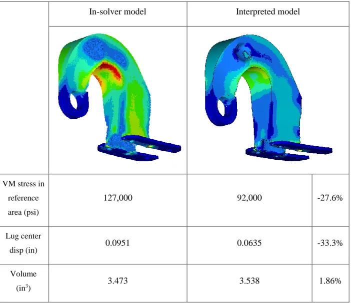
Table 3.1 – Performance and volume of an in-solver optimization result and its interpreted model. Volume of the latest is significantly lower than in-solver which leads to higher stress level and displacement. The iso-density filter was 0.75. ... 42

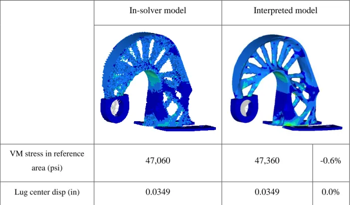
Table 3.2 – Example 1. Performance and volume difference between in-solver and interpreted models with iso-density filter at 0.5065. ... 44

Table 3.3 – Example 2. Performance and volume difference between in-solver and interpreted models. ... 46

Table 3.4 – Example 3. Performance and volume difference between in-solver and interpreted models. ... 48

Table 3.5 – Comparison between geometry from optimization result, mesh-based modeling and feature-based modeling. Interpretation time is significantly shorter when interpreted with mesh-based software. The red arrow shows where one bolt has not been considered during partial interpretation with mesh-based software. ... 53

Table 3.6 – Performance of optimization results and its interpretations ... 54

Table 3.7 – Loads applied on forward hinge ... 58

Table 3.8 – Loads applied on aft hinge ... 59

Table 3.9 – Material allowable at 200F for FE analyses ... 60

(11)

Table 3.11 – Margins of safety of the aft hinge ... 64

Table 3.12 – Lug margins of safety of the forward hinge ... 64

Table 3.13 – Lug margins of safety of the aft hinge ... 64

Table 3.14 – Margins of safety of bolts on forward hinge ... 65

Table 3.15 – Margins of safety of bolts on aft hinge ... 65

Table 3.16 – Partial interpretation methodology with SIMP and LSM ... 69

Table 3.17 – Comparison between two similar models optimized with SIMP (left) and LSM (right) on different computers ... 70

Table 3.18 – Comparison between original design and LSM optimizations done with volume target and stress target ... 71

Table 4.1 – Original (left) and optimized (right) demonstration models made in aluminum by additive manufacturing ... 73

Table 4.2 – Ti-6Al-4V AMS4928 element content tolerance ... 78

Table 5.1 – Summary of the results and their interests for the industrial partner and for professional development of the author ... 80

Table A.1 – Mechanical properties of wrought annealed Ti-6Al-4V titanium [36] ... 89

Table A.2 – Lugs parameters ... 92

Table A.3 – allowable on each lug ... 97

Table A.4 – Axial and transverse components of the forward hinge loads ... 98

Table A.5 – Axial and transverse components of the aft hinge loads ... 98

Table A.6 – Margins of safety of the forward hinge ... 100

Table A.7 – Margins of safety of the aft hinge ... 100

Table A.8 – CBUSH stiffness properties ... 101

Table A.9 – Bolts strength analyses from finite element model results ... 102

(12)

Table C.2 – Margin of safety of original part ... 110 Table C.3 – Optimization results are compared to simplified model of the original part (see Figure

C.2). ... 111 Table C.4 – Results of static finite element analysis on original part, smoothing interpretation,

CAD interpretation and results from setup 2. Original model results are from the complete model (see Figure 2). ... 113

(13)

LIST OF FIGURES

Figure 2.1 – Proportion of units sold above 5000$USD in 2014 by each machine manufacturers ... 12 Figure 2.2 – Growth and overall revenues of the additive manufacturing industry of the last 20

years ... 13 Figure 2.3 – Proportion of typical usage of additive manufacturing ... 14 Figure 2.4 – Industrial sectors in which AM is mostly used according to machine manufacturers

and service provides ... 14 Figure 2.5 – Topology optimizations of 2D beam using material density approach. The optimal

topology lies within its design space [16] ... 17 Figure 2.6 – Influence of penalization factor on relative stiffness. Adapted from [18]. ... 19 Figure 2.7 – Topology optimization of a 2D L-shape beam with stress constraints [24]. The stress

concentration is not avoided with global method in Optistruct (left) whereas a radius is created at the corner with clustered method in TRINITAS (right). ... 23 Figure 2.8 – 2D example with boundary represented by all the points on the level set surface at

time (t) equals k [29]. ... 24 Figure 2.9 – Level set optimization of the two-bar example with a perforated initial design [26] 25 Figure 3.1 – Design methodology with topology optimization ... 26 Figure 3.2 – Case study 1: flap track fitting in the trailing edge of a business aircraft ... 27 Figure 3.3 – Case study 2: APU door hinge of the CSeries commercial aircraft ... 28 Figure 3.4 – Case study 3: APU door hinge in the Global 7000/8000 business aircraft. Lugs are

pointed by the red arrow ... 28 Figure 3.5 – Original assembly of the flap with the outboard fitting with all the surrounding

components ... 29 Figure 3.6 – Design space for optimization of the outboard fitting with pockets for surrounding

(14)

Figure 3.7 – Design space used for CSeries APU door hinge. ... 30 Figure 3.8 – Result from optimization with an iso-density filter that keeps only elements with

density above 0.07. It is clear that density of elements is too low to be relevant. ... 31 Figure 3.9 – Design space (left) and result from topology optimization (right) of Global APU hinge.

The iso-density filter is at 0.6. ... 32 Figure 3.10 – Results from same optimization configuration done with fine elements (left) and

coarse elements (right) ... 32 Figure 3.11 – Extracted from [16]. Mesh refinement and dependency of results ... 33 Figure 3.12 – CSeries hinge with load components inducing bending (pink arrow) and torsion (blue

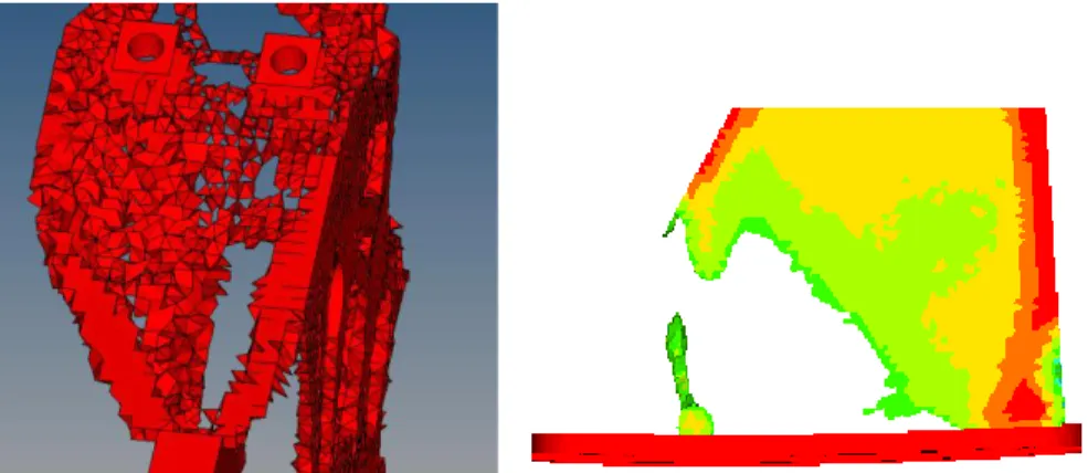
arrow) in the part ... 33 Figure 3.13 – Two models with different number of elements. The model on the left with fewer

elements is not accurately transferring torsion in the structure thus leading to an underestimated displacement value compared to the model on the right with finer mesh. ... 34 Figure 3.14 – Results from topology optimization with poor torsion stiffness due to large average

size of elements not accurately transferring moments in the structure ... 35 Figure 3.15 – On the left: design space with the ultimate load in pink. On the right: optimization

result with a bending node exactly where bending efforts vanish, i.e. aligned with the load. ... 36 Figure 3.16 – Load has been rotated downward so it is not aligned with the design space ... 37 Figure 3.17 – Boundary conditions too stiff can lead to unrealistic optimization results ... 37 Figure 3.18 – Design space of the track fitting with boundary conditions modeled as non-design

space with RBE3 and CBUSH to give a relative stiffness to the model ... 38 Figure 3.19 – Cseries hinge optimization with two models (left colomn). Upper model has a contact

condition at its base and the lower one does not. Both optimization gave similar results (right column). ... 39 Figure 3.20 – Elements to avoid in an optimization result: checkerboard pattern (left) and

(15)

Figure 3.21 – Two optimization results with same configuration but the model on the right has a symmetry constraint which led to a result with a lot of intermediate density elements ... 41 Figure 3.22 – Example 1. Difference between in-solver and interpreted volume with theoretical

zero volume difference at iso-density filter = 0.5065. ... 43 Figure 3.23 – Proportion of elements in each density bracket of the optimization result from

example 1 ... 45 Figure 3.24 – Proportion of elements in each density bracket of optimization result from example

2 ... 46 Figure 3.25 – Example 2. Difference between in-solver and interpreted volume. One can note that

the volume difference is within 5% from iso-density filter between 0.1 and 0.7 ... 47 Figure 3.26 – Example 3. Difference between in-solver and interpreted volume ... 49 Figure 3.27 – Example 3. Proportion of elements in each density bracket of optimization result 49 Figure 3.28 – Examples of bad geometry following the filtering by iso-density ... 50 Figure 3.29 – Validation and interpretation cycle of a topology optimization result ... 51 Figure 3.30 – Design space of the flap track fitting and its optimization result ... 51 Figure 3.31 – Element density distribution of the flap track fitting topology optimization result . 52 Figure 3.32 – Influence of final interpreted volume vs the chosen iso-density filter ... 52 Figure 3.33 – Optimization of the Global APU door hinge from the design space to the

interpretation ... 55 Figure 3.34 – Free-shape optimization of a section at the foot of the part. Nodes in the red (top left)

area are moved to minimize the stress (top right). ... 56 Figure 3.35 – Free-shape optimization of stress peak to lower the stress below the 100ksi limit . 56 Figure 3.36 – Load coordinate system of forward hinge ... 57 Figure 3.37 – True stress vs true plastic strain for Ti-6Al-4V at 200F ... 60 Figure 3.38 – Assembly of the hinge with stiffeners underneath (left) and FEA model with

(16)

Figure 3.39 – Finite element models of the forward (left) and aft (right) optimized hinges ... 61

Figure 3.40 – C1B (ult.) maximum stress zone on forward hinge ... 62

Figure 3.41 – C11B’ Maximum stress zone on aft hinge ... 63

Figure 3.42 – Results of the track support optimizations with different single point constraints configurations giving unrealistic stress distributions ... 67

Figure 3.43 – Optimization results with SIMP method where iso-density filtering produces irrelevant features ... 68

Figure 3.44 – Results from optimization with SIMP (left) and LSM (right). ... 68

Figure 4.1 – S-N curve of AMS4928 titanium coupons with surface finish of 100-125 Ra and 40-63 Ra ... 75

Figure 4.2 – Forward hinge with its fixture to ensure the test machine applies the loads in the desired orientation ... 76

Figure 4.3 – Numerical render with a testing fixture (blue) with virtual mating surface (yellow) with the hinge (green) ... 77

Figure 4.4 – Signed Von Mises stress of the hinge with a 1,952 lbf load magnitude ... 78

Figure A.1 – Ramberg-Osgood curve and complete engineering stress-strain curve of Ti-6Al-4V [36] ... 90

Figure A.2 – Material data points at room temperature and at 200F ... 91

Figure A.3 – True stress vs true plastic strain for Ti-6al-4v @200F ... 91

Figure A.4 – Dimensions of the forward (left) and aft (right) hinges ... 92

Figure A.5 – diagram of lug section ... 92

Figure A.6 – Lug axial loading failures ... 93

Figure A.7 – Axial tensile failure factor of Ti-6Al-4V ... 94

Figure A.8 – Axial shear-bearing failure factor ... 95

Figure A.9 – Axial yield factor ... 95

(17)

Figure A.11 – Load diagram of the loads in the elements of the lug assembly ... 99 Figure A.12 – Fasteners between hinges and base plate are represented by RBE2 and CBUSH 101 Figure C.1 – Model view of flap assembly ... 108 Figure C.2 – complete (right) finite element model will be used to validate the final designs only

and the simplified (left) model will be used to perform the topology optimization study. ... 109 Figure C.3 – Design space of the outboard fitting in the flap assembly (left) and isolated view

(right). ... 109 Figure C.4 – Finite element model (first on the left) and Von Mises stress contour of load case 1

(second) and load case 2 (third) of the outboard fitting. The part was first analyzed with the simplified model. ... 110 Figure C.5 – Results from optimization 7 and 8 with thin features and checkerboard effect... 111 Figure C.6 – Optimization 2 gave the most satisfactory results and is used for interpretation .. 111 Figure C.7 – Comparison between results out of the optimization solver (left) and after smoothing

in Blender (right) ... 112 Figure C.8 – Damaged elements around bolts due to sculpting in Blender ... 112 Figure C.9 – Intepretation of optimization setup 2 in Catia V5 ... 112 Figure C.10 – Von Mises stress distribution from finite element analyses of the original and the

optimized models for load case 1, the most severe. Ultimate tensile strength of Ph13-8Mo steel is 208,000psi. ... 113

(18)

LIST OF SYMBOLS AND ABBREVIATIONS

AM Additive Manufacturing

LPBF Laser powder-based fusion

MMPDS Metallic Material Properties Development and Standardization TO Topology optimization

SIMP Solid Isotropic Material Penalization

CRSNG Conseil National de Recherche en Sciences Naturelles et Génie du Canada FRQNT Fond de Recherche du Québec – Natures et Technologies

(19)

LIST OF APPENDICES

Appendix A – Global APU hinge analyses calculations ... 89 Appendix B – Test Matrix of qualifications coupons ... 106 Appendix C – Article 1: Paper of partial interpretation submitted to the Canadian Aeronautic and

(20)

CHAPTER 1 INTRODUCTION

This master’s thesis gathers 30 months of work conducted jointly with Bombardier Aerospace and Polytechnique Montréal. Thanks to the Industrial Innovation Scholarship Program from NSERC and FRQNT, the author worked on the integration of additive manufacturing (AM) technologies on productions parts at Bombardier Aerospace.

Additive manufacturing processes are defined, as the name suggests, by the fact that they build parts by adding material without mold or tooling. It is opposed to subtractive methods such as machining or other methods that require molds, e.g. casting or forging. AM methods therefore have a great geometrical freedom which allows to produce complex parts that wouldn’t be possible or very expensive otherwise.

In fact, now, in the aerospace industry, manufacturability dominates the design process. Thus, conservative compromises are made when considering efficient load bearing. In other words, manufacturing constraints of conventional methods limit the complexity of the structure which leads to heavier parts.

Therefore, designing parts solely in order to accomplish certain functions, such as bearing loads, instead of ensuring manufacturability, could help taking a lot of weight off an aircraft. With AM, this would be feasible but design methods and tools need to be revised.

Simulation tools such as finite element analysis (FEA) help predicting the performance of a part. With the increasing computing power available in the industry, FEA becomes standard and widely accepted as a stress validation method. Recent technologies can now even help predicting mathematically the optimal shape or topology of a part at the very beginning of the design life cycle. This is referred to as topology optimization.

Nevertheless, aerospace industry showed little interest in topology optimization since it creates parts with “organic” features that are hard if not impossible to manufacture. With AM, those parts could finally be manufactured with ease and yield the associated weight saving.

First AM processes were invented more than 30 years ago but the recent interest of Bombardier aerospace for producing parts with these technologies is motivated by several indicators.

(21)

Among other things, penetration of AM is significantly growing in the manufacturing sector for many consecutive years which partly testifies the capacities of the processes. More specifically, sales of AM machines rose significantly among other aerospace companies. Publicly released case studies demonstrate the intense investment in AM of the aerospace sectors, whether in military, civil or space.

Numerous elements also indicated that properties of metallic AM parts were sufficient to produce them steadily with great mechanical properties. Anterior research project showed that mechanical properties of titanium made in AM are close to these of regular wrought titanium. Moreover, several industrial suppliers were identified and some had relevant aeronautic experience which increases the level of confidence of their quality controls. Machine manufacturers improved the quality control of the machines themselves, helping to monitor defects in situ.

Stability of the supply chain also improved drastically during the last 3 to 5 years. In aerospace, large production requires stable and various suppliers. For instance, powder manufacturers specialized in raw powder for AM machines appeared recently. In addition, actual aerospace suppliers started to buy and use AM machines. Having suppliers with solid knowledge of the standard and quality requirements of the aerospace industry is a key aspect identified by Bombardier to invest in this area.

Furthermore, normalization organizations recently started to produce standards for processes, powders and mechanical testing which will ease qualification and certification of AM parts. However, at Bombardier, several challenges needed to be tackled in order to integrate additive manufacturing processes with the associated positive effects. In fact, very limited experience with numerical tools such as topology optimization previously existed. Design with simulation had been used only to optimize machined or forged parts. Moreover, full-size components were never produced using AM. Scalability risks and qualification needed to be addressed.

Ultimately, being able to scale the benefits of AM at Bombardier aerospace implies to have experts, called knowledge owners, able to identify areas where the technology could be integrated successfully. This requires to build practical experience and establish identification mechanisms among a focus group.

The present project was led by the Core Engineering - Structure department and partly financed by the Strategic Technology department. The role of the latter is to explore new technologies and

(22)

assess Technology Readiness Level (TRL) [5] of technologies that can potentially improve their products in different ways. On the other hand, the role of the Core Engineering – Structure department focuses specifically on improving the design and fabrication methods of the structures and their components. Depending on the TRL gate in which a certain technology is situated and the interest for Bombardier Aerospace, the scope of the projects will vary from technological surveillance to integration into production.

In the case of additive manufacturing, the readiness level was judged as sufficiently high to explore process qualification, a prerequisite to integration into production. However, all supporting areas of this manufacturing process such as design methodologies needed to be addressed. Therefore, a project was launched with several stakeholders from different engineering areas to cover: part selection, cost evaluation, supply chain, quality, design and stress. Those last two are the subject of this work. The presence of graduate students is favorable in this context since it allows to have a theoretical approach and explore with complete freedom the possibilities of the technologies. The first hypothesis that led the project was that additive manufacturing and use of numerical design tools such as topology optimization can lead to lighter products and therefore, more competitive aircrafts. The second hypothesis was that it is possible to qualify AM parts with short schedule and low resources. Indeed, integration of new manufacturing processes are historically resource and time extensive but with a new approach this could be reduced significantly.

Therefore, the first objective was to develop a methodology to design for additive manufacturing with the help of topology optimization. The second objective was to explore the qualification of additively manufactured parts in the aerospace industry with the associated qualification challenges with limited testing.

Although recent research has increased its 3 dimensional capacities, topology optimization was always used as a tool to benchmark concepts. Yet several challenges needed to be addressed in order to use this numerical technique to produce detailed designs. Exploration of topology optimization limitations and capabilities was done on 3 case studies of conventionally manufactured aeronautic parts. General guidelines are extracted at the different steps of the design lifecycle with topology optimization for additive manufacturing.

Few studies cover the complex venture of interpreting an optimization result. In this work, new approaches are proposed at the interpretation stage of the design to increase the level of confidence

(23)

of an optimization result and reduce the interpretation time. Moreover, a quick overview of the next generation of topology optimization solvers is introduced including novel algorithms such as the level-set method. This allows to assess the potential of the near-coming technologies in that field.

Moreover, no publicly available document covers the qualification of an AM part in aerospace. Design lifecycle in civil aviation includes material and process qualification. In this work, an affordable and rapid method to integrate a specific AM part on a civil aircraft is proposed. That’s why, in this study, to validate numerical analyses done on one of the aforementioned optimization case studies, a complete campaign of qualification tests was led. Qualifying a simple part requires low amount of resources and putting it into production then allows to accumulate statistical data over time which contributes to raising the confidence level of the whole process.

The following study is snapshot in time of two technologies in one industry at a specific point in time. It is foreseen that these findings will need to be updated in a few years when the technologies will get more mature.

(24)

CHAPTER 2 LITERATURE REVIEW

2.1 Design and qualification in aerospace

The design of aircrafts in the civil aerospace industry is regulated by national agencies. In Canada, Transport Canada “establishes and regulates standards for aeronautical products designed and operated in Canada” [1].

For detailed metallic components, specific rules exist related to their function, location or flight criticality in the aircraft. On the other hand, some general rules apply to all load bearing components. One of the most critical rule for certification is the stress criterion, stating that all components should not reach failure of the material at ultimate load and should not exceed plastic deformation at limit load.

The stress requirements are critical when designing parts for additive manufacturing because the properties of the material are not yet thoroughly established. On the other hand, for metallic parts machined out of wrought billets for example, material databases are complete enough to list statistical scatter of properties and subsequently extract material allowable. Those allowable are then used when analyzing the parts to ensure the stress level is below what’s permissible. In aerospace, the most common material database referred to is the Metallic Material Properties Development and Standardization [2] (MMPDS), which is approved by Transport Canada and the Federal Aviation Administration as well as the NASA in the US. However, no allowable is yet available in the MMPDS for additive manufactured materials, therefore, requiring other avenues for certification.

Since the development of an aircraft is driven by safety requirements, adding new components or technologies requires extensive testing. It is therefore often faster and more economical to copy already approved designs instead of finding new ways of improving parts.

Moreover, since the most predominant manufacturing technique nowadays is still machining, several constraints need to be taken into consideration during the design phase. Complex geometries that the machining tools cannot easily produce become expensive to produce if not downright impossible. This significantly limits the design freedom and instead of creating a part optimized for its functions such as bearing loads, it is designed to ease manufacturing.

(25)

As it is exposed in the following sections, additive manufacturing allows a great geometrical freedom that allows to align the design on the functions.

2.2 Additive manufacturing

Additive manufacturing, or 3D printing, is a family of manufacturing techniques characterized by the fact that material is bound together. The ASTM F42 committee in charge of normalizing additive manufacturing defines the latter as a “process of joining materials to make objects from 3D model data, usually layer upon layer, as opposed to subtractive manufacturing methodologies” [3] such as carving, drilling, machining, etc. Although a distinction is made between AM and 3D printing by the F42 committee, in general, both terms are used as synonyms.

As of 2015, ASTM F2792 divides all the AM technologies into 7 categories, detailed at Table 2.1 [3] [4].

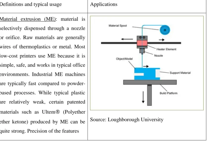
Table 2.1 – Categories of additive manufacturing technologies with their benefits and limitations Definitions and typical usage Applications

Material extrusion (ME): material is selectively dispensed through a nozzle or orifice. Raw materials are generally wires of thermoplastics or metal. Most low-cost printers use ME because it is simple, safe, and works in typical office environments. Industrial ME machines are typically fast compared to powder-based processes. While typical plastic are relatively weak, certain patented materials such as Ultem® (Polyether ether ketone) produced by ME can be quite strong. Precision of the features

(26)

Table 2.1 – Categories of additive manufacturing technologies with their benefits and limitations (continued)

made in ME depends on the wire and is therefore rougher than other processes. Additionally, delamination between layer is frequent. Used for affordable prototyping, larger machines are popular for building tools and molds.

Material jetting (MJ): droplets of material are selectively deposited and cured by an energy source, generally UV lights. This is one of the most precise process with moderate build speed. The ability to produce multi-material is a notable advantage of this technology. Mechanical properties are lower than other processes and often degrades after time due to light sensitivity. It is used

(27)

Binder jetting (BJ): liquid bonding agent is selectively deposited to join powder materials. All kind of powders can be used (plastics and metals). Bonding agent can be replaced in a post-processing operation by low viscosity metals such as gold, brass, etc. Only sintering of material is achievable with this technology and thus, low mechanical properties must be expected. Typical applications are plugs for

casting, filters and jewelry. Source: Loughborough University Sheet lamination (SL): a laser or a

robotized knife cuts a layout in multiple sheets of paper. The sheets are then bonded together to form an object. Colors can be printed on the paper prior to cut of the layout. This process is affordable and allows to make model with a complete palette of colors. However, it is slow and parts made by SL have very low mechanical properties.

(28)

Vat photopolymerization (VP): liquid photopolymer in a vat is selectively cured by light-activated polymerization. This was the first 3D printing process to be invented. It remains the most precise technique and offers acceptable mechanical properties. Many types of resins can be used while many sizes of machines at different prices exist. However, the process is expensive to run since uncured resin is often wasted. Typical applications are functional prototypes, custom medical devices (tooth braces, hearing aids, etc.) and investment casting plugs.

Source: Loughborough University

Powder bed fusion (PBF): thermal energy selectively fuses regions of a powder layer. Once the powder is consolidated, the build platform goes down, another layer of powder is dropped on top of the previous one by a powder roller and the process starts over. Thermoplastics and metals with good weldability can be manufactured. This technique offers a good precision on dimensions but this is variable

(29)

depending on the material. Mechanical properties are comparable to other processes. It is probably the most economical technology. Metallic parts made in PBF are generally used in medical, aerospace and oil & gas industries.

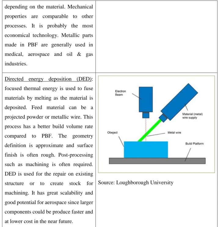
Directed energy deposition (DED): focused thermal energy is used to fuse materials by melting as the material is deposited. Feed material can be a projected powder or metallic wire. This process has a better build volume rate compared to PBF. The geometry definition is approximate and surface finish is often rough. Post-processing such as machining is often required. DED is used for the repair on existing structure or to create stock for machining. It has great scalability and good potential for aerospace since larger components could be produce faster and at lower cost in the near future.

Source: Loughborough University

According to Wohlers Associates [5], the AM technologies market can be divided in 2 sectors: industrial grade machines and consumer “desktop” machines selling for less than 5000$USD. This last category is mostly constituted of material extrusion machines and won’t be discussed in this work.

(30)

2.2.1 Growth and recent development

As of 2015, the largest industrial AM machines manufacturers in terms of units sold are Stratasys from Israel, 3D Systems from the USA and Envisiotech from Germany. EOS from Germany could be added to this group as it is the leading powder-bed fusion machine manufacturer and whose notable growth illustrates the interest for this technology. Figure 2.1 and Table 2.2 below picture the financial results and the importance of the larger machine manufacturers.

Table 2.2 – Most important AM machine manufacturers in the world and their accumulated sales and revenues in 2014 [6].

Companies Technologies Units sold since

1990 Revenues in 2014 (USD$) Stratasys Material extrusion 41869 750M Material Jetting 3D Systems Vat photopolymerization 17792 654M

Polymer powder-bed fusion Metal powder-bed fusion

Binder jetting Material jetting Material extrusion EnvisioTech Vat photopolymerization 5878 Undisclosed (around 100M) (bio) Material extrusion

EOS

Polymer powder-bed fusion

1762 195M

(31)

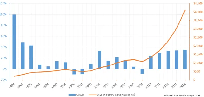
Figure 2.1 – Proportion of units sold above 5000$USD in 2014 by each machine manufacturers Additive manufacturing industry including revenues of products (sales of machines, materials, software, etc.) and services (production of parts by service providers, maintenance, training, etc.) trade around the world has been increasing rapidly for the last 20 years. According to Wohlers Associates [5], the most renowned AM consulting firm in the world, since 2010, compound annual growth rate (CAGR) of AM industry is above 20%, with a record of 35.2% in 2014.

Figure 2.2 shows the overview of the revenues and CAGR of this industry for the past 20 years. Numbers exclude the sales relative to the desktop 3D printed machines.

(32)

Figure 2.2 – Growth and overall revenues of the additive manufacturing industry of the last 20 years

Historically, AM was mostly used for prototyping purposes. The fast turnovers allow to iterate rapidly on a design without having to invest in tooling just for prototypes. The cost of AM production was previously too high to be cost-effective in actual production. Moreover, the limited materials available 10 to 20 years ago made it hard to get the desired results. However, the technologies have now matured and the most popular applications for AM have shifted from prototyping towards functional parts, although prototyping still remains the most frequent application, as depicted in Figure 2.3.

(33)

Figure 2.3 – Proportion of typical usage of additive manufacturing

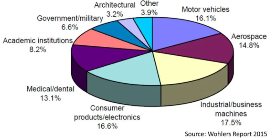
Almost all manufacturing industries and many services industries are now using AM somewhere in their business model. Figure 2.4 illustrates the distribution of customers per industry according to 127 of the largest AM machine manufacturers and AM service providers across the world.

Figure 2.4 – Industrial sectors in which AM is mostly used according to machine manufacturers and service provides

Among all industries, aerospace is probably the most interested in AM and its potential applications. Indeed, high-value components and low production volume constitutes an ideal scenario for AM. Boeing engineers stated that they already installed around 100,000 AM parts on 16 of their commercial and military aircrafts. Although most of those parts were in polymers, the interest for metal parts made by powder-bed fusion is increasing. Table 2.3 gathers some examples of metal parts for aerospace applications that were publicly demonstrated from 2013 to 2015.

(34)

Table 2.3 – Publicly released AM aerospace applications

General Electric

Fuel nozzle for LEAP engine, combining 18 parts into 1 while being 25% lighter and lasting 5 times longer. In 2015 only, 30,000 units will be produced [7].

Airbus

Cabin bracket, optimized by topology optimization. It flew on Airbus’ new A350 in June 2014. The part is reported as 30% lighter than its machined counterpart [8].

SpaceX

Falcon 9 Rocket main oxidizer valve. It was originally casted but powder-bed fusion allowed to have greater material properties and a manufacturing lead time of 2 days instead of months [9].

Aerojet Rocketdyne

Bantam demonstration motor entirely produced with 3 powder-bed fusion parts assembled together allowed to consolidate dozens of parts together. The cost of the motor was reduced by 65% [10].

(35)

Table 2.3 – Publicly released AM aerospace applications (continued)

GKN Aerospace

Leading edge concept component optimized by topology optimization and built by powder-bed fusion. Several sub-components were combined in the final part [11].

2.2.2 Selective laser melting process

Powder-bed fusion process, as explained before, melts powder to consolidate a part. The energy required to this aim can be provided by a laser (laser powder-bed fusion, LPBF) or an electron beam (electron beam powder-bed fusion). Although the electron beam technology has its advantages and is promising, the present work focuses on LPBF. Particularly, the material that is of interest in this work is the titanium Ti-6Al-4V (60% of titanium production in USA and EU). Due to its raw price 10 times higher than aluminum for instance [12], titanium is often avoided in civil aviation, despite its interesting mechanical and thermal properties [2].

As an exotic and new manufacturing process, AM can be quite expensive and has a narrow window for good business cases. However, considering the potential weight saving of an optimized design and the high cost of machining titanium, producing parts in titanium by AM can be competitive.

2.3 Topology optimization

One of the greatest interest of aerospace for AM is the ability to design products with few manufacturing constraints on the geometry. Thus, it allows to get designs optimized to meet certain

(36)

performance targets such as weight or aerodynamic properties instead of optimizing manufacturability.

In order to do so, numerical tools exist that help predicting what is the best material distribution within a volume to optimize certain criteria while respecting defined constraints. The most popular algorithm for this is called topology optimization (TO). Based on finite element models, TO solvers can be well integrated into the design methodology in aerospace. Several TO algorithms exist but focus is placed on the more mature which are already used commercially. In this study, for its applicability to the aerospace industry, only TO software able to optimize 3D parts (volume) will be considered and the one prominently used is Optistruct by Altair.

2.3.1 Solid Isotropic Material Penalization (SIMP) Method

Rozvany [13] classifies the different topology optimization approaches in the following categories: Isotropic Solid/Empty (ISE), Anisotropic Solid/Empty (ASE) and Isotropic Solid/Empty/Porous (ASEP). More specifically, the ISE approach includes the Solid Isotropic Material Penalization method (SIMP) which is in 2015, the most commonly used in commercially available software. 2.3.1.1 Homogenization of density

One can argue that topology optimization started at the end of the 1980s with the paper of Bendsoe and Kikuchi [14]. Before that, most of the research efforts in numerical structures optimization where concentrated on shape optimization. In two papers published in 1988 and 1989 [15], Bendsoe proposed a method, later coined as Solid Isotropic Material Penalization (SIMP). This numerical method is based on the idea that the optimal material distribution of a structure can be comprised within a bigger volume called the design space. By discretizing the design space in elements, some elements can be turned on or off so they contribute or not to the overall stiffness of the structure. Therefore, in finite element modeling, every element is a design variable that can be either solid (turned on) or a void (turned off), see Figure 2.5 below.

Figure 2.5 – Topology optimizations of 2D beam using material density approach. The optimal topology lies within its design space [16]

(37)

However, in practice, the discrete nature of the solid/void concept is numerically hard to handle. Thus, Bendsoe [15] proposed the material density approach which works with continuous variables that are easier to compute. The stiffness equation, where 𝑓 is the external forces vector applied on the structure, 𝐾 the stiffness matrix and 𝑢 the displacement vector is:

𝑓 = 𝐾 ∙ 𝑢 ( 1 )

The stiffness matrix can be written as:

𝐾 = 𝐾(𝜌(𝑥)) = (𝜌𝑒(𝑥)) 𝑝

𝐾𝑒 ( 2 )

Where 𝜌𝑒(𝑥) is a density function varying between 0 and 1 for all design variables (elements) denoted as 𝑥. Thus, the stiffness 𝐾 can vary continuously between 0 and 𝐾_𝑒, the actual stiffness of the material.

An ideal solution would have all the densities at either 0 or 1 since intermediate stiffness don’t have any physical meaning with homogenous materials. Thus, the exponent 𝑝 over the density function is introduced to penalize intermediate density values. It is repeated in the literature that 𝑝 = 3 works well [17].

Figure 2.6 illustrates the influence of the penalization factor on the relative stiffness of the element. As 𝑝 increases, intermediate values of density are closer to either 0 or 1.

(38)

Figure 2.6 – Influence of penalization factor on relative stiffness. Adapted from [18]. 2.3.1.2 Sensitivity analysis

The SIMP method is gradient-based, meaning it evaluates sensitivity of the responses to changes of the design variables. For example, if a design variable, in this case an element of the model, contributes in increasing the stiffness of the model, its density is raised. Otherwise, density of the element decreases until it eventually vanishes. This is important since most mathematical numerical algorithms are based on sensitivity analyses. Thus, optimizations can be formulated with different objectives and constraints (minimize compliance, reduce displacement, reduce weight, etc.) and sensitivity of all these parameters with the design variables shall be established. The general mathematical formulation of an optimization problem being of the following form:

min ℎ(𝑥) ( 3 )

𝑔_𝑖(𝑥) ≤ 𝐺 ; 𝑖 = 1, … , 𝑚 ( 4 )

Where ℎ(𝑥) is the objective function, i.e.: the response to be optimized, and 𝑔_𝑖(𝑥) are the 𝑚 constraints to be respected. In numerical optimization, the responses are all the monitored output such as compliance, stress, displacement, etc. Most of the possible responses are related to displacement 𝑢(𝑥) (see stiffness equation above). Therefore, sensitivity analysis of all responses are often derived from sensitivity between displacement and design variables:

(39)

𝜕ℎ(𝑥, 𝑢(𝑥))

𝜕𝑥𝑗 𝑓𝑜𝑟 𝑗 = 1, … , 𝑛

Where 𝑥𝑗 is a design variable and 𝑛 the total number of design variables (i.e. number of elements). In problems with large amounts of design variables such as most topology optimization problems, the response function sensitivity is found by the adjoint variable method [16]. Instead of calculating the displacement sensitivity for all variables and for each response, the adjoint method allow to compute sensitivity for all variables once for each response, significantly reducing the calculation time.

2.3.1.3 Formulations

Several optimization methods can be used to solve topology optimization problems but the details will not be explained in this work. Here’s a short list of the most commonly used optimization methods:

 Optimality criteria (OC), reviewed and explained in details in the book of Bensoe [16].  Method of moving asymptotes (MMA) or convex linearization (CONLIN) which are both

similar. The former, proposed by Svanberg in 1987 [19] is based on the later by Fleury and Braibant in 1985 and 1989 [20]. The idea is to divide the domain into smaller sections where the optimization function will be convex and where a linearization is possible. This is probably the most widely used method in numerical topology optimization.

 Method of feasible directions (MFD), initially proposed by Vanderplaats in 1983 [21]. 2.3.1.4 Responses

The standard optimization formulation is the following:

min ℎ(𝑥) =1₂𝑓𝑇_𝑢(𝑥) _{( 5 )}

with

(40)

where 𝑣_𝑒 is the volume of an element and the function ℎ(𝑥) is the compliance. The variable 𝑓 is the external load vector and 𝑢(𝑥) is the displacement vector. Compliance is inversely proportional to stiffness thus measuring the flexibility of a structure. Therefore, the objective is to reduce the compliance (increasing stiffness) with a limited amount of volume 𝑉. Compliance is an interesting response to work with since it is closely related to displacement and its sensitivity is greatly simplified by the adjoint method.

2.3.1.5 Stress driven optimization

When topology optimization is used as a design tool, several factors need to be considered such as stress distribution in the structure. Indeed, in an industrial context, the design of parts is often driven by the acceptable stress level. Thus, depending on the material used, a maximum stress level is to be respected.

𝜎𝑒 < 𝜎̅̅̅̅̅; ; 𝑒 = 1, … , 𝑁 𝑉𝑀 ( 7 ) Where 𝜎_𝑒 is the stress measured in element 𝑒 and 𝜎̅̅̅̅̅ is, for example, the maximum Von Mises _𝑉𝑀 stress allowable by the material. Adding this constraint in the formulation of the optimization results in adding one stress constraint for each element, or design variable in the model. This is in practice totally impossible to use as it would be too time-consuming to compute sensitivity for each constraint.

Another problem with stress constraint is the singularity problem. For example, with a bar in tension, as the diameter of the bar decreases, its stress level increases. In an optimization problem, this would prevent the bar (or element) to vanish.

The stress penalization method has been studied by several authors to avoid the singularity problem [22]. The idea is to penalize the stress the same way the stiffness is penalized.

𝜎_𝑒 = 𝜌_𝑒(𝑥)𝑞_𝜎 𝑒

̂ ; 𝑒 = 1, … , 𝑁 ( 8 )

Thus, the calculated stress level of an element 𝜎_𝑒 decreases if the density of the element vanishes, even if the actual stress level 𝜎̂ increases. Exponent 𝑞 helps again inforcing intermediate value 𝑒 elements toward 0 or 1.

To reduce the number of design variables when optimizing a problem with local stress constraints, several techniques can be used but few have been successfully implemented in a commercial solver.

(41)

A popular technique is to use a global constraint, where only the elements with the highest stress level are considered in the optimization. Initially proposed by Werme in 2008 [23], this technique is not efficient in avoiding stress concentrations.

A recent clustering technique developed by Holmberg [24] proposes a promising compromise between global and local constraints that is worth being mentioned. The idea is to group all the elements with similar stress level in clusters where only one stress constraint will be computed for each cluster. To do this, all the measured stress points are placed in descending order.

𝜎₁ ≥ 𝜎₂ ≥ 𝜎₃ ≥ ⋯ ≥ 𝜎𝑛𝑎 𝑛𝑖 ⏟ 𝑐𝑙𝑢𝑠𝑡𝑒𝑟 1 ≥ ⋯ ≥ 𝜎2𝑛𝑎 𝑛𝑖 ⏟ 𝑐𝑙𝑢𝑠𝑡𝑒𝑟 2 ≥ … ≥ 𝜎𝑋𝑛𝑎 𝑛𝑖 ⏟ 𝑐𝑙𝑢𝑠𝑡𝑒𝑟 𝑋 ≥ … ≥ 𝜎⏟ _𝑛𝑖−1 ≥ 𝜎_𝑛𝑖 𝑐𝑙𝑢𝑠𝑡𝑒𝑟 𝑛𝑖 ( 9 )

Where 𝑛𝑎 is the number of stress measured points and 𝑛𝑖 the number of clusters. Then, a constraint is extracted from the cluster with a P-norm averaging.

( 10 ) Where 𝜎_𝑖 is the stress constraint for cluster 𝑖 (Ω_i), 𝜎_𝑎 the stress measured at points contained in Ω_i and 𝑝, a predetermined factor. As factor 𝑝 increases, the value of 𝜎_𝑖 gets closer to the maximum stress measure point of the cluster (max

𝑎𝜖Ω𝑖 𝜎𝑎(𝑥)). Holmberg reports using values for 𝑝 between 8

and 12.

A comparison between the clustered and the global techniques is illustrated in Figure 2.7 where an L-shape beam is optimized with two different stress constraint techniques: global and clustered. The global stress constraint being too rough, it cannot get rid of the stress concentration in the corner as opposed to the clustered stress constraint where a radius is created to smooth the concentration. The latter has been implemented in the TRINITAS solver.

(42)

Figure 2.7 – Topology optimization of a 2D L-shape beam with stress constraints [24]. The stress concentration is not avoided with global method in Optistruct (left) whereas a radius is created at the corner with clustered method in TRINITAS (right).

However, Holmberg shows that the clustered approach can be much more time-consuming than the global approach.

2.3.2 Level Set

The level set method (LSM) was first introduced by Osther and Sethian [25] to study front propagation under a speed vector, such as lava dripping down along the contour of a volcano. Its adaptation to topology optimization was initially proposed by Wang [26] and Allaire [27]. The fundamental principle of the level set method for topology optimization are briefly described here but for further information, the reader is referred to the review by Van Dijk et al. [28].

The level-set method can be exemplified with a 2D contour moving along a surface. The idea is to implicitly represent the boundary S with a higher dimension model 𝜑(𝑥, 𝑡), where 𝑥 is the coordinate vector, 𝑡 is the virtual time, representing boundary variations. Therefore, as illustrated in Figure 2.8, the 2D space hatched in red is represented as the contour of a 3D surface at a certain value of 𝑡 = 𝑘. Points 𝑥 that belong on the boundary are defined by the iso-contour S that intersect the level set model at height 𝑘.

(43)

Figure 2.8 – 2D example with boundary represented by all the points on the level set surface at time (t) equals k [29].

The boundary is defined with the following relation:

𝜑(𝑥) {

> 0 𝑖𝑓 𝑖𝑛𝑠𝑖𝑑𝑒 𝑏𝑜𝑢𝑛𝑑𝑎𝑟𝑦 = 0 𝑖𝑓 𝑜𝑛 𝑏𝑜𝑢𝑛𝑑𝑎𝑟𝑦 < 0 𝑖𝑓 𝑜𝑢𝑡𝑠𝑖𝑑𝑒 𝑏𝑜𝑢𝑛𝑑𝑎𝑟𝑦

( 12 )

Using partial derivative of the surface, the level set can be modified to satisfy a certain objective under certain constraints (e.g. minimizing compliance with a maximum volume). As shown in Figure 2.9, during the optimization, holes in the level set can vanish or be combined with each other. However, new holes cannot be created. Therefore, the original solutions proposed by Wang [26] is to introduce holes in the design space.

(44)

Figure 2.9 – Level set optimization of the two-bar example with a perforated initial design [26] This method is design dependent and several authors have published methods to avoid the artificial introduction of holes in the design space with topological derivatives [30] [31] or with the evolutionary “hard-kill” method [29].

Complexity of the LSM is proportionate to the surface it describes rather than the volume it encapsulates, which makes it more efficient at dealing with problems with large number of degrees of freedom. Furthermore, the level set model does not homogenize the density of elements. Thus, stiffness of the resulting topologies is more accurate and, as it is exposed later, interpretation is easier.

Level set method is highly scalable and can be used for 3D models. As of 2016, several commercial software incorporate topology optimization with the level set method and some exploratory work with this method is exposed in Section 3.4.

(45)

CHAPTER 3 DESIGN METHODOLOGY FOR ADDITIVE

MANUFACTURING

The rationale of this work focuses on part replacement. The approach is different than a clean sheet design and it is often a much harder task as well. Indeed, when a part is replaced, there is no flexibility on the surrounding space which limits the available choices. Complementary to this, when the boundary conditions are fixed there is less room for optimization of the load paths. However, succeeding to design a proper replacement part is a clear proof that topology optimization make sense even in difficult scenarios. Moreover, as an earlier exploration of this technology, there are less risks to design new parts a posteriori, meaning it is outside of the engineering master schedule during the development of an aircraft.

Nonetheless, it is believed that the greatest usage of topology optimization with additive manufacturing parts in aerospace would be at the early stages of development where there is more flexibility on all components.

Figure 3.1 illustrates the different steps in order to design a part with topology optimization. In the following sections, those steps will be explored with their opportunities and limitations.

(46)

3.1 Topology optimization

The results obtained with topology optimization are dependent on what is done at each of the steps. They are mostly independent but to certain extent, some choices at a particular step limit the others. There is no such thing as a unique recipe that will work every time in every situation. However, there are things to favor and to avoid when configuring a topology optimization. Failing to do so can lead to unsatisfactory optimization results. The first part of this chapter is dedicated to the description of good practices in configuring a topology optimization.

Furthermore, even when satisfactory results are obtained, it is a challenge to objectively select which result is best. Additionally, the following step, i.e. to interpret this finite element result into an aerospace part, is the subject of many research work in the optimization community. In the later portion of this chapter, a new approach will be detailed on how partial interpretation introduced in the actual methodology can help increasing the pace of the design lifecycle.

Throughout this thesis, 3 case studies will be exposed to illustrate the findings. They are presented in no particular order. The last case study on the auxiliary power unit (APU) door hinge of the Global aircraft will also be the sole subject of Chapter 4.

The first case deals with a fitting that supports the flap track in the trailing edge of a business aircraft, see Figure 3.2. This part is made in corrosion resistant steel and is riveted to the wing and bolted to track of the flap. Therefore, it is a highly critical part bearing large stress levels. Moreover, the part is large (14in x 6in x 12in) compared with the other two. This case study remains theoretical and never intended to be produced by ALM since it is too large for all the commercial PBFL machines currently available.

(47)

The second part studied here is illustrated in Figure 3.3. It is the hinge attaching the door of the auxiliary power unit (APU) in the CSeries, a commercial airplane. Built out of titanium for its strength at 200ºF and 400ºF, the CSeries’ hinge has an arched geometry to allow a clearance when opening the door. The arch connects to a single lug. The loading scenarios involve in severe conditions such as 200F temperature with some surrounding components that have failed. Moreover, the part is bolted to a composite door which is less tolerant to impacts than a metallic one. Therefore, although they are normally small during regular operating conditions, the design loads are pretty high.

Figure 3.3 – Case study 2: APU door hinge of the CSeries commercial aircraft

The third case study focuses on a part with the same functions than the previous one but in a different aircraft. In the Global 7000 and 8000 aircrafts, although smaller than the CSeries, the APU door hinge is larger with dual lugs, see Figure 3.4. This part is an older design and therefore much heavier and bulkier than the CSeries’ one. Design loading scenarios are similar to the second case.

Figure 3.4 – Case study 3: APU door hinge in the Global 7000/8000 business aircraft. Lugs are pointed by the red arrow

(48)

3.1.1 Configuration

In a part replacement approach, modeling the design space can be more complex compared to a situation where no component is yet fixed in the environment of the part. Thus, as the example in Figure 3.5 shows, the design space of the flap track fitting has to nest between several other components. Moreover, fixation of the fasteners has to be considered, including their installation.

Figure 3.5 – Original assembly of the flap with the outboard fitting with all the surrounding components

In the numerical model, a non-design space has also to be set. This is the area that needs to be kept fully dense and therefore cannot be modified. Critical features of the part are often important to put as non-design space since their integrity is not calculated by FEA. For example, lugs and areas around bolts which are designed according to empirical equations must be preserved. Figure 3.6 shows design space in green and non-design spaces in yellow for the optimization model of the flap track fitting.

(49)

Figure 3.6 – Design space for optimization of the outboard fitting with pockets for surrounding elements and fasteners. Design space is in green, non-design space in yellow.

One can think that the larger the design space, the better are the chances to capture the right topology. However, in practice, it is often the opposite. Too large design spaces can lead to results with very low density elements. In Figure 3.7, the illustrated design space used for the CSeries APU hinge is much bigger than the original part: 32.8in3 vs. 2.4in3 respectively.

Figure 3.7 – Design space used for CSeries APU door hinge.

(50)

In order to obtain a weight reduction, in this example, more than 93% of the elements must have a density of 0. However, in practice, convergence of low density elements is never perfect and a lot of elements with medium density value appear, like it is exposed in Figure 3.8. Those elements bias the results by increasing artificially the stiffness according to Equation (2).

Later, when the geometry is interpreted and low density elements deleted, the stiffness will be much different. This dichotomy between in-solver results and interpreted results is addressed later.

Figure 3.8 – Result from optimization with an iso-density filter that keeps only elements with density above 0.07. It is clear that density of elements is too low to be relevant.

Thus, targeting low volume fraction (below 15%) implies that most of the elements should be around 0. Therefore, the design space has to be narrowed down around the most probable area so the targeted volume fraction is high enough.

The design space of the Global APU hinge illustrated in Figure 3.9 is a good example of all the elements mentioned above. The areas around fasteners are set as non-design spaces to prevent them to be altered. The design space has been reduced near the foot of the part to allow a clearance to install fasteners. Also, the design space is of reasonable size so there are fewer mid-density elements present in the result.

(51)

Figure 3.9 – Design space (left) and result from topology optimization (right) of Global APU hinge. The iso-density filter is at 0.6.

3.1.2 Meshing

Meshing of the model can have a significant influence on the results but the effect can be reduced if a handful of general rules are followed. The parameters to control when meshing a topology optimization model are the size and the type of elements.

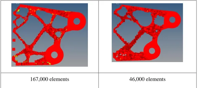
The resulting topology from an optimization is directly influenced by the average size of elements in its model. Results from the same models but with different average elements sizes are illustrated in Figure 3.10. It can be seen that the model with smaller elements has finer features that could not be revealed when elements are larger.

167,000 elements 46,000 elements

Figure 3.10 – Results from same optimization configuration done with fine elements (left) and coarse elements (right)