HAL Id: hal-01957628
https://hal.laas.fr/hal-01957628
Submitted on 17 Dec 2018
HAL is a multi-disciplinary open access
archive for the deposit and dissemination of
sci-entific research documents, whether they are
pub-lished or not. The documents may come from
teaching and research institutions in France or
abroad, or from public or private research centers.
L’archive ouverte pluridisciplinaire HAL, est
destinée au dépôt et à la diffusion de documents
scientifiques de niveau recherche, publiés ou non,
émanant des établissements d’enseignement et de
recherche français ou étrangers, des laboratoires
publics ou privés.
3D Leaf Tracking for Plant Growth Monitoring
William Gélard, Ariane Herbulot, Michel Devy, Pierre Casadebaig
To cite this version:
William Gélard, Ariane Herbulot, Michel Devy, Pierre Casadebaig. 3D Leaf Tracking for Plant Growth
Monitoring. 25th IEEE International Conference on Image Processing (ICIP 2018), Oct 2018, Athènes,
Greece. 5p. �hal-01957628�
3D LEAF TRACKING FOR PLANT GROWTH MONITORING
William G´elard
?‡Ariane Herbulot
?Michel Devy
†Pierre Casadebaig
‡?
LAAS-CNRS, Universit´e de Toulouse, UPS, F-31400 Toulouse, France
†LAAS-CNRS, Universit´e de Toulouse, CNRS, F-31400 Toulouse, France
‡AGIR, Universit´e de Toulouse, INRA, F-31326 Castanet-Tolosan, France
ABSTRACT
This article presents a 3D approach in plant growth monitor-ing and deals with the trackmonitor-ing of leaves of sunflower plants. Our aim is to compute time-series of individual leaf area, un-der water stress and control conditions. These data will then be used by biologists to study the drought resistance of vari-ous sunflower species. Our method to track the leaves in 3D has been evaluated on a set of 132 point clouds obtained via classical structure-from-motion techniques and multi-view stereo software. These 3D acquisitions have been performed on 12 sunflower plants (6 water-stressed, 6 well-watered) during a period of one month (11 measurement dates per sun-flower plant). This method gives promising results for both conditions (water-stressed and well-watered), for different species and is able to follow the growth of the plants, as well as to detect new leaf emergence and leaf decay.
Index Terms— 3D leaf tracking, plant monitoring, time tracking, labelling, 3D plant phenotyping, Sunflower plants.
1. INTRODUCTION
In order to increase food production through improved crop performance, research in plant breeding focus on relation-ships between genotype (DNA) and phenotype (visual char-acteristics). While genotyping methods are rapidly improv-ing, most of the current phenotyping methods are manual, invasive and sometimes destructive. In order to fill the gap between genotype and phenotype data, phenotyping was re-cently linked with automation and signal processing to in-crease its throughput [1, 2]. Aiming to study drought resis-tance of sunflower plants, a key plant’s characteristic under a changing climate, the French National Institute for Agri-cultural Research has developed a semi-controlled outdoor phenotyping platform allowing agronomists and geneticists to monitor up to 1300 plants in pots and control the water stress of each plant.
Recent studies pointed the use of 3D data in order to au-tomatically extract visual characteristics of a plant instead of 2D images because the main limitations in 2D come from oc-clusions due to overlappings between leaves [3, 4, 5]. In 3D the problem still persist but few examples have shown that
the use of Structure from Motion is well adapted in 3D plant digitalization and reconstruction and can be used for 3D plant phenotyping [4, 5]. We previously addressed 3D reconstruc-tion and 3D model-based segmentareconstruc-tion in [6, 7] (1) to obtain a 3D model of a plant and (2) to extract the stem, and to seg-ment, label and compute the area of every leaf.
The problem addressed here, monitor the leaves during the plant growth, reveals a great challenge in following a live object in 3D like a sunflower plant, that grow in an unpre-dictable way and remains a major problem in plant phenotyp-ing. To meet this challenge, we work on plant growth in pot in a semi-controlled outdoor phenotyping platform. The starting point of our labelling method is a 3D point cloud of a sun-flower plant already segmented. We start by isolating a plant and take about hundred images around it, under controlled light illumination and wind condition. Then we use classical structure from motion techniques and multi-view stereo soft-ware like OpenMVG [8] and PMVS/CMVS [9, 10] in order to reconstruct the plant in 3D [6]. After cleaning the point cloud, we apply a stem extraction algorithm in order to ease the leaves segmentation by using an Euclidean cluster extrac-tion as detailed in [7].
This paper is focused on the leaves tracking during the plant growth, it introduces a labelling method that allows to track the leaves over times. It is organized as follows: sec-tion 2 presents our method to track the leaves during the plant growth. Section 3 shows the results obtained on a set of 12 sunflower plants during a period of one month and finally, section 4 draws conclusions on the use of this method and provides guidelines for further works.
2. METHOD
As our main objective is to follow the expansion rate of leaf areas on sunflower plants during their growth, we have turned the problem into a 3D object tracking over time, applied to track the leaves. To reach this aim, we have developed a method with (1) an initial labelling step relying on the botan-ical model of a sunflower plant that allows to assign a unique label to each leaf, (2) a label propagation step that allows to track the leaves, making sure that these labels do not change
Stem × A × A0 Leaf A × B ×B 0 Leaf B
(a) Front view
A B A0, B0 Stem Leaf A Leaf B × × × α (b) Top view
Fig. 1. Description of divergence angle computation
over time, and (3) the detection of new leaf emergence and of old leaf decay.
We will present how we design our labelling method to follow leaves over time, introducing the sunflower phyllotaxy, that describes the way how leaves appear and are organised along the stem. First, we will detail the initial labelling step used to assign a unique label to every leaf, and then the prop-agation step used to follow leaves over time.
2.1. Leaves labelling 2.1.1. Plant phyllotaxy
The main function attributed to phyllotaxy is to increase the ability of the plant to intercept light for photosynthesis by minimizing cast shadows between leaf layers. The arrange-ment of leaves appears as regular and is the result of bio-chemical control during the leaf appearance and expansion. The emergence of leaves respects particular rules proper to each specie. Two types of phyllotaxy are observed: cyclic and spiral ones. If there is only one leaf per node (term used to express where leaves appear on the stem), it is a spiral ar-rangement, if there are two leaves or more per node, it is a cyclic arrangement as explained in [11, 12]. In the cyclic phyllotaxy, the leaves at each node form a whorl with constant angles between leaves. In a spiral leaf arrangement, a single leaf is attached to a particular node on the stem, leaves are distributed around the stem in a spiral pattern. A plant with a spiral arrangement consistently has a symmetrical pattern with the exact same number of leaves for each turn around the stem. The angle between two successive leaves around the stem is called, divergence angle. It represents how a new leaf on the plant stem is positioned with respect to the previ-ous one. This divergence angle is always constant but differ between species [13].
In sunflower plants, two types of phyllotaxy were identi-fied, depending on the leaf position on the stem: the first three pairs of leaves are organized with a cyclic phyllotaxy
(oppo-Algorithm 1: Initial leaves labelling input : Leaves
output: Leaves labelled
1 // Sort the leaves by the height of their insertion point 2 sort(leaves);
3 foreach (leaf in leaves) do 4 nextLeaf ← leaf.next; 5 thirdLeaf ← nextLeaf.next;
6 if (nextLeaf.height ' thirdLeaf.height) then 7 α1= divergenceAngle(leaf, nextLeaf ); 8 α2=
divergenceAngle(leaf, thirdLeaf );
9 if (α2− 137.5◦< α1− 137.5◦)then 10 swap(nextLeaf, thirdLeaf);
11 end
12 end 13 end
site decussate, successive leaf pairs are 90◦apart), while from the leaf 7, it appears a spiral phyllotaxy with an angle of di-vergence α = 137.5◦. The first pairs decay quickly in favour of the ones arranged in spiral [14].
2.1.2. Initial leaves labelling
Knowing that the main sunflower phyllotaxy is spiral, i.e., there are only one leaf per node, the first idea was to sort the leaves by the height of their insertion point along the stem and to assign them a label according to this order. The leaf at the bottom will receive the label 0, the next one, the label 1 and so on. Moreover, knowing that the theoritical divergence angle for a sunflower plant is α = 137.5◦, we used it in order to detect potential labelling errors. The divergence angles are always computed in the counter-clockwise direction as shown in Figure 1 and with the following equation:
α = (
arccos( ~LA· ~LB) if det( ~LA, ~LB) ≥ 0
360 − arccos( ~LA· ~LB) otherwise
(1)
where ~LA& ~LB means Leaf A & Leaf B and the
determi-nant det( ~LA, ~LB) is used to detect the angle orientation. In
[6] we have shown that this divergence angle might not re-spect the model when two leaves have close insertion points on the stem. If it is the case, labels of these two leaves need to be swapped in order to get a divergence angle that respects the model.
All these observations have lead to the Algorithm 1, which is used as an initial labelling step for each sunflower plant. The next step, is to verify these labels by propagating the ones obtained at the previous acquisition, checking and correcting them in order to ensure that every leaf keeps the same label during the plant growth period.
Algorithm 2: Labels propagation input : Previous divergence angles output: First label
1 sumAngle ← 0;
2 foreach (angle in previousDivergenceAngle) do 3 sumAngle ← sumAngle + angle; 4 //Check angle modulo (2π)
5 if (αref − sumAngle < −toleranceAngle) then 6 αref ← αref+ 360;
7 end
8 //Compare angle
9 if ( sumAngle − αref < toleranceAngle) then
10 Correspondance found; 11 end
12 end
2.2. Labels propagation
Our main objective is to monitor the plant growth, usually during a month. We perform a 3D acquisition every 2, 3 or 4 days and apply our initial leaves labelling algorithm to each plant from its 3D reconstruction. During the monitoring pro-cess, we always take care to perform the acquisition with the same plant orientation. We compute the divergence angle of the first leaf with the x-axis in order to get the orientation of the plant. We call this angle, the referential divergence angle (αref). Here the main problem comes from the growth of the
plant itself, as our labelling method relies on the height of the leaf insertion points on the stem. Knowing that the inter-node distance grows uncertainly depending on the plant environ-ment (light illumination, water, temperature...), it is possible that two leaves close at a certain time, are distant from each other at another time, making their label switched. Moreover, the first leaves can decay and disappear and new leaf can ap-pear in an unexpected way.
In order to detect and address these kind of events, we propagate the labels obtained at the previous acquisition (ex-cept for the initial acquisition where there is no previous la-bel). First, we have developped the Algorithm 2 in order to compare the referential divergence angle with the one ob-tained at the previous acquisition to retrieve the label of the first leaf, as well as to detect potential leaf decay. Then, we compare the other divergence angles in order to check if no la-bel have been switched. The divergence angles are compared with a certain tolerance to be invariant against uncertainty and noise related to the 3D reconstruction and segmentation.
3. RESULTS
In order to evaluate the accuracy and repeatability of our method, we have performed a test on a set of 12 sunflower plants from 2 different species, 6 plants have been placed
under water stress condition and 6 under control condition (well-watered). The test was performed during autumn 2017, between the beginning of September till mid-November with 3D aquisitions made every 2, 3 or 4 days for a total of 11 ac-quisitions per plant and a full amount of 132 point clouds of sunflower plants. An example of 3D plant growth monitoring is given in Figure 2, where we can see that the leaves keep the same labels during the monitoring period1.
3.1. Segmentation
As the starting point of our method is a 3D sunflower plant, where the leaves have already been segmented, we present the segmentation results obtained on a set of 132 point clouds. In most cases, plants have been successfully segmented, only 4 point clouds have not been well segmented, which represents 3% of faillure. Moreover, these failure only appears for the plants at an advanced stage of water stress. For each well seg-mented plant, 80% of the leaves have been retrieved and the 20% missing are the small leaves that are appearing under the top of the plant (the capitulum), but as shown in [6], we as-sumed that the smaller leaves (under the top) do not contribute strongly to light interception and plant functioning and so, are not considered in the phenotyping method.
3.2. Initial leaves labelling
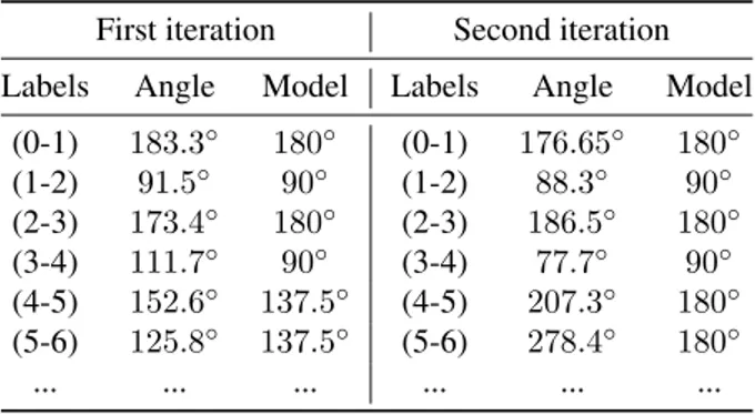
For the initial leaves labelling step, due to the particular phyl-lotaxy of the sunflower plant (opposite phylphyl-lotaxy following by a spiral one), if the leaves that appear in pairs are still present when we start the acquisition, it is difficult to deter-mine which leaf is the first. In order to solve this issue, we execute the Algorithm 1 twice, swapping the label of the two first leaves between the execution. This gives two configura-tions and we have to select the one that respect the phyllotaxy of a sunflower plant. An example is given in the table 1 where it is possible to see the result associated to the acquisition made during the first date Day 1. Here, the first iteration gives the best solution. This method was able to label all the seg-mented leaves in our set of 132 point clouds, for the 2 species and in both conditions (water-stressed and well-watered).
3.3. Labels propagation
The aim of the labels propagations step is two-fold: (1) prop-agate the previous label in order to find the correct label of the first leaf as well as to detect potential leaf decay and (2), check that all the divergence angles are in accordance with the previous ones in order to make sure that labels have not changed.
In order to illustrate the problem of leaf decay, we present in Table 2 results obtained for a plant where two leaves have
1This paper has supplementary examples provided by the authors. It
in-cludes two videos showing the monitoring of a stressed and a well irrigated plant during their growth. This material is 12.7 MB in size.
(a) Day 1 (b) Day 15 (c) Day 17 (d) Day 28
Fig. 2. Plant growth monitoring
First iteration Second iteration Labels Angle Model Labels Angle Model
(0-1) 183.3◦ 180◦ (0-1) 176.65◦ 180◦ (1-2) 91.5◦ 90◦ (1-2) 88.3◦ 90◦ (2-3) 173.4◦ 180◦ (2-3) 186.5◦ 180◦ (3-4) 111.7◦ 90◦ (3-4) 77.7◦ 90◦ (4-5) 152.6◦ 137.5◦ (4-5) 207.3◦ 180◦ (5-6) 125.8◦ 137.5◦ (5-6) 278.4◦ 180◦ ... ... ... ... ... ...
Table 1. Example of initial leaves labelling at Day 1
decayed 17 days after the first acquisition. In this table, we present the divergence angle available at the previous acqui-sition: Day 15. On Day 17, we have a referential divergence angle between the first leaf and the x-axis αref(17) = 51.3
◦.
We can retrieve the label associated to this leaf by comparing αref(17) with αref(15) and all the divergence angles on this
day. In this case:
αref(17) ' αref(15)+ α(0−1)(15)+ α(1−2)(15) (2)
= 134.6◦+ 195.7◦+ 83.2◦= 413.5◦ (3) = 53.5◦(2π) . (4) We can see that two leaves present at Day 15 (Figure 2(b)) have decayed and are no longer present at Day 17 (Fig-ure 2(c)), which means that the label of the first leaf available at this date is no longer 0 but 2. Our method works for our point clouds but has a limitation due to the use of a referential divergence angle (αref) computed between the first leaf and
the x-axis, plants have to be placed in the same orientation for the 3D acquisition during the monitoring period. In our dataset of 12 sunflower plants, the leaf decays appear at dif-ferent times according to the specie but the method was able to detect them.
4. CONCLUSION
In this paper we have presented a 3D approach for plant growth monitoring applied to sunflower plants. This approach
Day 15 Day 17
Labels Angle Angle Observation αref 134.6◦ 53.5◦ -α(0−1) 195.7◦ - Decay α(1−2) 83.2◦ - Decay α(2−3) 158.6◦ 164.4◦ √ α(3−4) 111.7◦ 110.2◦ √ ... ... ... ... α(11−12) - 124.5◦ New leaf α(12−13) - 149.9◦ New leaf
Table 2. Example of labels propagation
relies on our previous work made on 3D plant reconstruc-tion and segmentareconstruc-tion that was validated on sunflower and sorghum plants [6, 7]. The idea is to follow the plant growth of sunflower plants and especially, to follow the leaves over time. To do so, a labelling method has been developped relying on the phyllotaxy of sunflower plants. This method allows us to (1), follow each leaf individually by assigning a unique label that does not change over time and (2), to detect new leaf emergence and old leaf decay during the plant growth. This method was tested on a set of 12 plants with 11 acquisitions associated to each plant during a period of one month and has been proven to be robust enough to follow the leaves. After being able to follow the leaves during the plant growth, more work will be focused on computing leaves characteristics (e.g., area, color, curvature with the stem, etc), with the specific aim to determine if a leaf is still active or not. Here, the challenge might be solved by machine or deep learning, by training the system with annotated agronomist data.
5. ACKNOWLEDGEMENTS
The authors would like to thank Philippe Debaeke, Nicolas Langlade and Philippe Burger from INRA, for their participa-tion to this work, through a joint project about high through-put phenotyping of sunflower plants and the French National Research Agency through the project SUNRISE.
6. REFERENCES
[1] Stijn Dhondt, Nathalie Wuyts, and Dirk Inz´e, “Cell to whole-plant phenotyping: the best is yet to come,” Trends in Plant Science, vol. 18, no. 8, pp. 428–439, 2013.
[2] Fabio Fiorani and Ulrich Schurr, “Future Scenarios for Plant Phenotyping,” Annual review of plant biology, vol. 64, pp. 267–291, 2013.
[3] Ga¨etan Louarn, Serge Carr´e, Fr´ed´eric Boudon, Annie Eprinchard, and Didier Combes, “Characterization of whole plant leaf area properties using laser scanner point clouds,” in Fourth International Symposium on Plant Growth Modeling, Simulation, Visualization and Appli-cations, 2012.
[4] T. T. Santos and A. A. Oliveira, “Image-based 3D dig-itizing for plant architecture analysis and phenotyping,” in Workshop on Industry Applications (WGARI), 2012. [5] Sylvain Jay, Gilles Rabatel, Xavier Hadoux, Daniel
Moura, and Nathalie Gorretta, “In-field crop row phe-notyping from 3D modeling performed using Structure from Motion,” Computers and Electronics in Agricul-ture, vol. 110, pp. 70–77, 2015.
[6] William G´elard, Michel Devy, Ariane Herbulot, and Philippe Burger, “Model-based Segmentation of 3D Point Clouds for Phenotyping Sunflower Plants,” in Pro-ceedings of the 12th International Joint Conference on Computer Vision, Imaging and Computer Graphics The-ory and Applications, 2017, pp. 459–467.
[7] William G´elard, Ariane Herbulot, Michel Devy, Philippe Debaeke, Ryan F. McCormick, Sandra K. Truong, and John Mullet, “Leaves Segmentation in 3D Point Cloud,” in Advanced Concepts for Intelligent Vi-sion Systems. 2017, pp. 664–674, Springer International Publishing.
[8] Pierre Moulon, Pascal Monasse, Romuald Perrot, and Renaud Marlet, “OpenMVG: Open Multiple View Ge-ometry,” in Reproducible Research in Pattern Recogni-tion. 2017, Springer International Publishing.
[9] Yasutaka Furukawa, Brian Curless, Steven M. Seitz, and Richard Szeliski, “Towards Internet-scale Multi-view Stereo,” in CVPR, 2010.
[10] Yasutaka Furukawa and Jean Ponce, “Accurate, Dense, and Robust Multi-View Stereopsis,” IEEE Trans. on Pattern Analysis and Machine Intelligence, vol. 32, no. 8, pp. 362–1376, 2010.
[11] Samuel Boiss`ıere, “Dynamique de la Phyllotaxie,” 2000.
[12] Chrystel Feller, Christian Mazza, and Florence Yerly, “Plantes, spirales et nombre : les plantes font-elles des maths?,” Bulletin de la Soci´et´e Fribourgeoise des Sci-ences Naturelles, vol. 99, pp. 122–137, 2010.
[13] Soumendra Kumar, “Phyllotaxy (Arrangement of Leaves): Cyclic and Spinal Phyllotaxy,” .
[14] Herv´e Rey, Jean Dauzat, Karine Chenu, Jean-Franc¸ois Barczi, Guillermo A. A. Dosio, and J´er´emie Lecoeur, “Using a 3-D Virtual Sunflower to Simulate Light Cap-ture at Organ, Plant and Plot Levels: Contribution of Organ Interception, Impact of Heliotropism and Analy-sis of Genotypic Differences,” Ann Bot, vol. 101, no. 8, pp. 1139–1151, 2008.