HAL Id: inria-00176758
https://hal.inria.fr/inria-00176758
Submitted on 4 Oct 2007
HAL is a multi-disciplinary open access archive for the deposit and dissemination of sci-entific research documents, whether they are pub-lished or not. The documents may come from teaching and research institutions in France or abroad, or from public or private research centers.
L’archive ouverte pluridisciplinaire HAL, est destinée au dépôt et à la diffusion de documents scientifiques de niveau recherche, publiés ou non, émanant des établissements d’enseignement et de recherche français ou étrangers, des laboratoires publics ou privés.
communication
Wilfrid Perruquetti, Thierry Floquet, Emmanuel Moulay
To cite this version:
Wilfrid Perruquetti, Thierry Floquet, Emmanuel Moulay. Finite time observers: application to secure communication. IEEE Transactions on Automatic Control, Institute of Electrical and Electronics Engineers, 2008, 53 (1), pp.356-360. �10.1109/TAC.2007.914264�. �inria-00176758�
Finite time observers: application to secure
communication
Wilfrid Perruquetti, Thierry Floquet and Emmanuel Moulay
Abstract
In this paper, control theory is used to formalize finite time chaos synchronization as a nonlinear finite time observer design issue. This paper introduces a finite time observer for nonlinear systems that can be put into a linear canonical form up to output injection. The finite time convergence relies on the homogeneity properties of nonlinear systems. The observer is then applied to the problem of secure data transmission based on finite time chaos synchronization and the two-channel transmission method.
Index Terms
Finite time observers, finite time synchronization, two-channel transmission, secure communication.
I. INTRODUCTION
A lot of encryption methods involving chaotic dynamics have been proposed in the literature since the 90’s. Most of them consists of transmitting informations through an insecure channel, with a chaotic system. The synchronization mechanism of the two chaotic signals is known as chaos synchronizationand has been developed for instance in [1]. The idea is to use the output of the drive system to control the response system so that they oscillate in a synchronized manner.
W. Perruquetti and T. Floquet are with the LAGIS (UMR CNRS 8146), Ecole Centrale de Lille, Cité Scientifique, 59651 Villeneuve d’Ascq Cedex, France and with Centre de recherche INRIA futurs, Equipe Projet ALIEN. (e-mail: [email protected], [email protected])
E. Moulay is with IRCCyN (UMR-CNRS 6597), 1 rue de la Noë, B.P. 92 101, 44321 Nantes CEDEX 03, France (e-mail: [email protected])
Since the work [2], the synchronization can be viewed as a special case of observer design problem, i.e the state reconstruction from measurements of an output variable under the assump-tion that the system structure and parameters are known. This approach leads to a systematic tool which guarantees chaos synchronization of a class of observable systems. Different observer based methods were developed: adaptive observers [3], backstepping design [4], Hamiltonian forms [5] or sub-Lyapunov exponents [1]. Nevertheless, during the chaos synchronization of continuous systems, the convergence of the error is always asymptotic as in [6]. Instead of attempting the construction of an asymptotic nonlinear observer for the transmitter or coding system, a finite time chaos synchronization for continuous systems (in the sense that the error reaches the origin in finite time) can be developed. Finite time observers for nonlinear systems that are linearizable up to output injection have been proposed in [7] and [8] using delays or in [9] and [10] using discontinuous injection terms. Recently, an algebraic method (using module theory and non-commutative algebra) leading to the non asymptotic estimation of the system states has been developed in [11] and applied to chaotic synchronization in [12]. In this work, an homogeneous finite time observer is introduced. This observer yields the finite time convergence of the error variables without using delayed or discontinuous terms. Then, it is applied to the finite time synchronization of chaotic systems and combined with the conventional cryptographic method called two-channel transmission in order to design a cryptosystem. The technique of two channel transmission has been proposed in [13]. Other cryptography techniques for secure communications exist such as the parameter modulation developed in [14].
The paper is organized as follows. The problem statement and some definitions are given in Section II. An homogeneous finite time observer is developed in Section III. On the basis of this observer, a two-channel transmission cryptosystem is built and is applied in Section IV to the Chua’s circuit that is relevant to secure communications (see e.g. [15] and [16]).
II. PROBLEM STATEMENT AND DEFINITIONS
Let us consider a nonlinear system of the form:
˙x = η (x, u) (1)
where x ∈ Rd is the state, u ∈ Rm is a known and sufficiently smooth control input, and
y(t) ∈ R is the output. η : Rd× Rm → Rd is a known continuous vector field. It is assumed
that the system (1)-(2) is locally observable [17] and that there exist a local state coordinate transformation and an output coordinate transformation which transform the nonlinear system (1)-(2) into the following canonical observable form:
˙z = Az + f (y, u, ˙u, ..., u(r)) (3)
y= Cz (4)
where z ∈ Rn is the state, r ∈ N >0 and A= a1 1 0 0 0 a2 0 1 0 0 ... ... ... ... ... an−1 0 0 0 1 an 0 0 0 0 , C =³ 1 0 ... 0 ´ . (5)
The transformations involved in such a linearization method for different classes of systems with n = d can be found in [18], [19], [20], [21]. One can have n > d in the case of system immersion [22], [23].
Then, the observer design is quite simple since all nonlinearities are function of the output and known inputs. Asymptotic stability can be obtained using a straightforward generalization of a linear Luenberger observer. Finite time sliding mode observers have already been designed for system (3)-(4) (see e.g. [9], [10]). However, they rely on discontinuous output injections and on a step-by-step procedure that can be harmful for high order systems. In this paper, a finite time observer based on continuous output injections is introduced.
Notions about finite time stability and homogeneity are recalled hereafter. Finite time stability
Consider the following ordinary differential equation:
˙x = g (x) , x∈ Rn. (6)
Note φx0(t) a solution of the system (6) starting from x
Definition 1: The system (6) is said to have a unique solution in forward time on a neigh-bourhood U ⊂ Rn if for any x
0 ∈ U and two right maximally defined solutions of (6),
φx0 : [0, T
φ[ → Rn and ψx0 : [0, Tψ[ → Rn, there exists 0 < Tx0 ≤ min {Tφ, Tψ} such that
φx0(t) = ψx0(t) for all t ∈ [0, T
x0[.
Let us consider the system (6) where g ∈ C0(Rn), g(0) = 0 and where g has a unique solution
in forward time. Let us recall the notion of finite time stability involving the settling-time function given in [24, Definition 2.2] and [25].
Definition 2: The origin of the system (6) is Finite Time Stable (FTS) if:
1) there exists a function T : V \ {0} → R+ (V is a neighbourhood of the origin) such that
for all x0 ∈ V \ {0}, φx0(t) is defined (and unique) on [0, T (x0)), φx0(t) ∈ V \ {0} for all
t∈ [0, T (x0)) and lim t→T(x0)
φx0(t) = 0.
T is called the settling-time function of the system (6).
2) for all ǫ > 0, there exists δ (ǫ) > 0 such that for every x0 ∈ (δ (ǫ) Bn\ {0}) ∩ V, φx0(t) ∈
ǫBn for all t ∈ [0, T (x 0)).
The following result gives a sufficient condition for system (6) to be FTS (see [26], [27] for ODE, and [28] for differential inclusions):
Theorem 3: Let the origin be an equilibrium point for the system (6), and let r be a continuous function on an open neighborhood V of the origin. If there exist a Lyapunov function V : V → R+
and a function r : R+→ R+ such that
˙
V(x) ≤ −r(V (x)), (7) along the solutions of (6) and ε > 0 such that
Z ε 0
dz
r(z) <+∞, (8) then the origin is FTS.
The interested reader can find more details on finite time stability in [29], [30], [31], [32], [33], [34].
Homogeneity
Definition 4: A function V : Rn→ R is homogeneous of degree d with respect to the weights (r1, . . . , rn) ∈ Rn>0 if
V (λr1x
for all λ > 0.
Definition 5: A vector field g is homogeneous of degree d with respect to the weights (r1, . . . , rn) ∈
Rn
>0 if for all 1 ≤ i ≤ n, the i−th component gi is a homogeneous function of degree ri+ d,
that is
gi(λr1x1, . . . , λrnxn) = λri+dgi(x1, . . . , xn)
for all λ > 0. The system (6) is homogeneous of degree d if the vector field g is homogeneous of degree d.
Theorem 6: [25, Theorem 5.8 and Corollary 5.4] Let g be defined on Rnand be a continuous
vector field homogeneous of degree d < 0 (with respect to the weights (r1, . . . , rn)). If the origin
of (6) is locally asymptotically stable, it is globally FTS.
III. A CONTINUOUS FINITE TIME OBSERVER
Assume that the system (1)-(2) can be put into the observable canonical form (3)-(4). An observer for this system is designed as follows
dˆz1 dt ... dˆzn dt = A z1 ˆ z2 ... ˆ zn + f (y, u, ˙u, ..., u(r)) − χ1(z1− ˆz1) χ2(z1− ˆz1) ... χn(z1− ˆz1) (9)
where the functions χi will be defined in such a way that the observation error e = z − ˆz tends
to zero in finite time. Set e = h e1 e2 · · · en
iT
. The observation error dynamics is given by ˙e1 = e2+ χ1(e1) ˙e2 = e3+ χ2(e1) ... ˙en−1 = en+ χn−1(e1) ˙en = χn(e1) (10) Denote ⌈x⌋α
Lemma 7: Let d ∈ R and (k1, . . . , kn) ∈ Rn>0. Define (r1, . . . , rn) ∈ Rn>0 and (α1, . . . , αn) ∈ Rn >0 such that ri+1 = ri+ d, 1 ≤ i ≤ n − 1, (11) αi = ri+1 r1 , 1 ≤ i ≤ n − 1, (12) αn= rn+ d r1 , (13) and set χi(e1) = −ki⌈e1⌋αi, 1 ≤ i ≤ n.
Then, the system (10) is homogeneous of degree d with respect to the weights (r1, . . . , rn) ∈ Rn>0.
Proof of Lemma 7 is obvious. Denote α1 = α.
Lemma 8: If α > 1 − n−11 , the system (10) is homogeneous of degree α − 1 with respect to the weights {(i − 1) α − (i − 2)}1≤i≤n and αi = iα − (i − 1) , 1 < i ≤ n.
Proof: Let us normalize the weights by setting r1 = 1. Then r2 = α and
d = r2− r1 = α − 1.
From (11) and (12)-(13), one obtains recursively that:
ri = (i − 1) α − (i − 2) , 1 < i ≤ n,
αi = iα − (i − 1) , 1 < i ≤ n.
Since r1 > . . . > rn>0, one has:
α > n− 2
n− 1 = 1 − 1 n− 1. The result follows from Lemma 7.
The system (10) is then given by: ˙e1 = e2− k1⌈e1⌋α ˙e2 = e3− k2⌈e1⌋2α−1 ... ˙en−1 = en− kn−1⌈e1⌋(n−1)α−(n−2) ˙en= −kn⌈e1⌋nα−(n−1) (14)
denoted shortly
˙e = ψ(α, e). (15) Lemma 9 (Tube Lemma): Consider the product space X × Y , where Y is compact. If N is an open set of X × Y containing the slice {x0} × Y of X × Y , then N contains some tube
W × Y about {x0} × Y , where W is a neighborhood of x0 in X.
Theorem 10: Set the gains (k1, . . . , kn) such that the matrix
Ao= −k1 1 0 0 0 −k2 0 1 0 0 ... ... ... ... ... −kn−1 0 0 0 1 −kn 0 0 0 0 is Hurwitz. Then, there exists ǫ ∈ £1 − 1
n−1,1
¢
such that for all α ∈ (1 − ǫ, 1), the system (15) is globally finite time stable.
Proof: Set
1 − 1
n− 1 < α <1.
Homogeneity:From Lemma 8, the system (15) is homogeneous of degree α−1 < 0 with respect to the weight {(i − 1) α − (i − 2)}1≤i≤n.
Asymptotic stability: Consider the following differentiable positive definite function
V (α, e) = yTP y (16) where y= ⌈e1⌋ 1 q ⌈e2⌋ 1 αq ... ⌈ei⌋ 1 [(i−1)α−(i−2)]q ... ⌈en⌋ 1 [(n−1)α−(n−2)]q , q= n−1 Y i=1
((i − 1) α − (i − 2)) is the product of the weights and P is the solution of the following Lyapunov equation
As V is proper,
S = {e ∈ Rn: V (1, e) = 1}
is a compact set of Rn. Define the function
ϕ: R>0× S → R
(α, e) 7→ h∇V (α, e) , ψ(α, e)i Since Ao is Hurwitz, the system
˙e = Ao e
is globally asymptotically stable and corresponds to the system (15) with α = 1. Since ϕ is continuous, ϕ−1(R
<0) is an open subset of Λ×S containing the slice {1}×S. Since S is compact,
it follows from the Tube Lemma 9 that ϕ−1(R
<0) contains some tube (1 − ǫ1,1 + ǫ2) × S about
{1} × S. For all (α, e) ∈ (1 − ǫ1,1 + ǫ2) × S
h∇V (α, e) , ψ(α, e)i < 0.
Thus, the system (15) is locally asymptotically stable. It can also be shown to be globally asymptotically stable as follows. Note that
V (α, λr1e
1, . . . , λrnen) = λ
1
q2V (α, e
1, . . . , en)
with ri = (i − 1) α − (i − 2) for 1 ≤ i ≤ n. Thus
e7→ V (α, e) is homogeneous of degree 1
q2 with respect to the weights {(i − 1) α − (i − 2)}1≤i≤n. From [35],
it can be deduced that
e7→ h∇V (α, e) , ψ(α, e)i is homogeneous of degree 1
q2+ α − 1 with respect to the weights {(i − 1) α − (i − 2)}1≤i≤n and
thus is negative definite. This imply that, for α ∈ (1 − ǫ1,1 + ǫ2),
e7→ V (α, e) is a Lyapunov function for the system (15).
IV. CRYPTOSYSTEM AND ITS APPLICATION TO THECHUA’S CIRCUIT
Several chaotic systems, as the three-dimensional Genesio-Tesi system [36], the Lur’e-like system or the Duffing equation [37], belong to the class of systems (3-4). Let us show that the proposed observer can be useful to perform finite time synchronization of this class of chaotic systems and secure data transmission. For a two-channel transmission, the system governing the transmitter is given by:
˙z = A z + f (y) (17)
y= z1 (18)
s(t) = νe(z(t), m(t)) . (19)
The first channel is used to convey the output y = z1 of the chaotic system (17). The function
νe encrypts the message m (t) and delivers the signal s (t) which is transmitted via the second
channel. The receiver gets z1(t) on the first channel. An observer is designed as follows:
dˆz1 dt ... dˆzn dt = A z1 ˆ z2 ... ˆ zn + f (y) + On(y − ˆz1) (20) where On(y − ˆz1) = k1⌈z1− ˆz1⌋α k2⌈z1− ˆz1⌋2α−1 ... kn⌈z1− ˆz1⌋nα−(n−1) .
The error dynamics e = z − ˆz is given by the system (15). With a good choice of α and {ki}1≤i≤n, Theorem (10) implies that the error dynamic e (t) converges to the origin in finite
time. As a consequence, the message m (t) can be completely recovered after the finite time synchronization by the system
System (20) ˆ y= ˆz1 ˆ m= νd(ˆz, s) .
The Chua’s circuit belongs to the class of chaotic systems which can be put into the observable canonical form. (3)-(4) The equations of a Chua’s oscillator are given by:
C1˙x1 = R1 (x2− x1) + h (x1) C2˙x2 = R1 (x1− x2) + x3 L˙x3 = −x2− rx3 (21) where L is a linear inductor, R and r two linear resistors, C1 and C2 two linear capacitors,
h(x) = G2x1+12(G1− G2) (|x1+ B| − |x1 − B|)
is the piecewise linear Chua’s function. The chosen output is y = x1.
Using the transformation z = T x with T = 1 0 0 1 C2R+ r L 1 C1R 0 1 C2L¡1 + r R ¢ r C1LR 1 C1C2R
the system (21) is transformed into the observable canonical form (17)-(18) with A= −C11R − C12R− r L 1 0 −L1 ³ r C1R+ r C2R + 1 C2 ´ 0 1 −1 C1C2RL 0 0 , f(y) = 1 C1 1 C1 ³ 1 C2R + r L ´ 1 C1C2L¡1 + r R ¢ h(y) .
In the simulations, the numerical values of the Chua’s circuit are C1 = 10.04 nF, C2 = 102.2
nF, R = 1747 Ω, r = 20Ω, L = 18.8 mH, G1 = −0.756 mS, G2 = −0.409 mS, H = 1 V.
The gains of the observer have been set as follows: α = 0.7, k1 = 1000, k2 = 240, k3 = 24. The
observation error dynamics e = z − ˆz is then given by ˙e1 = e2− 1000 ⌈e1⌋0.7 ˙e2 = e3− 240 ⌈e1⌋0.4 ˙e3 = −24 ⌈e1⌋0.1 . (22)
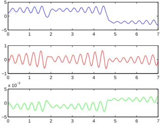
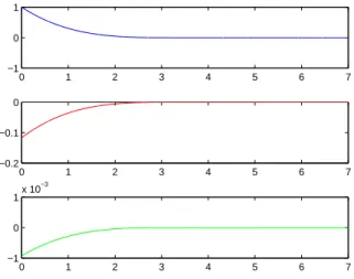
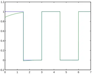
and e (t) converges to the origin in finite time (see Fig. 1 and 2). A message m (t) can be sent and recovered after the delay due to the finite time synchronization by using the previous algorithm (see Fig. 3).
0 1 2 3 4 5 6 7 −5 0 5 0 1 2 3 4 5 6 7 −1 0 1 0 1 2 3 4 5 6 7 −5 0 5x 10 −3
Fig. 1. State of the system (21) and its estimate
Remark 11: It is possible to increase the security of the transmission by introducing some observation singularities in the system (17). In this case, finite time convergence is a useful property (see [38]).
V. CONCLUSION
In this paper, a continuous finite time observer based on homogeneity properties has been designed for the observation problem of nonlinear systems that are linearizable up to output injection. It does not involve any discontinuous output injections and step-by-step procedure, as it is the case, for instance, for sliding mode observers. It has been applied to finite time chaos synchronization and to secure data transmission using the two-channel transmission method.
REFERENCES
[1] L. M. Pecora and T. L. Carroll, “Synchronization in chaotic systems,” Phys. Rev. Lett., vol. 64, pp. 821–824, 1990. [2] H. Nijmeijer and I. M. Y. Mareels, “An observer looks at synchronization,” IEEE Trans. Circuits Systems I Fund. Theory
Appl., vol. 44, no. 10, pp. 882–890, 1997.
[3] A. Fradkov, H. Nijmeijer, and A. Markov, “Adaptive observer-based synchronization for communication,” Internat. J. Bifur. Chaos Appl. Sci. Engrg., vol. 10, no. 12, pp. 2807–2813, 2000.
[4] S. Mascolo and G. Grassi, “Controlling chaos via backstepping design,” Phys. Rev. E (3), vol. 56, no. 5, pp. 6166–6169, 1997.
0 1 2 3 4 5 6 7 −1 0 1 0 1 2 3 4 5 6 7 −0.2 −0.1 0 0 1 2 3 4 5 6 7 −1 0 1x 10 −3
Fig. 2. Observation error
[5] D. López-Mancilla, C. Cruz-Hernández, and C. Posadas-Castillo, “A modified chaos-based communication scheme using hamiltonian forms and observer,” Journal of Physics: Conference Series, vol. 23, pp. 267–275, 2005.
[6] G. Grassi and S. Mascolo, “Nonlinear observer design to synchronize hyperchaotic systems via a scalar signal,” IEEE Trans. Circuits Systems I Fund. Theory Appl., vol. 44, no. 10, pp. 1011–1014, 1997.
[7] R. Engel and G. Kreisselmeier, “A continuous-time observer which converges in finite time,” IEEE Trans. Automatic Control, vol. 47, no. 7, pp. 1202–1204, 2002.
[8] F. Sauvage, M. Guay, and D. Dochain, “Design of a nonlinear finite-time converging observer for a class of nonlinear systems,” Journal of Control Science and Engineering, 2007.
[9] S. V. Drakunov and V. I. Utkin, “Sliding mode observers. tutorial,” 1995.
[10] W. Perruquetti, T. Floquet, and P. Borne, “A note on sliding observer and controller for generalized canonical forms,” in IEEE Conference on Decision and Control, Tampa, Florida, USA, 1998, pp. 1920 – 1925.
[11] M. Fliess and H. Sira-Ramírez, “Reconstructeurs dŠetat,” C. R. Acad. Sci. Paris Sér. I Math., vol. 338, pp. 91–96, 2004. [12] H. Sira-Ramírez and M. Fliess, “An algebraic state estimation approach for the recovery of chaotically encrypted messages,”
Internat. J. Bifur. Chaos Appl. Sci. Engrg., vol. 16, pp. 295–309, 2006.
[13] Z. P. Jiang, “A note on chaotic secure communication systems,” IEEE Trans. Circuits Systems I Fund. Theory Appl., vol. 49, no. 1, pp. 92–96, 2002.
[14] T. Yang and L. Chua, “Secure communication via chaotic parameter modulation,” IEEE Trans. Circuits Systems I Fund. Theory Appl., vol. 43, no. 9, pp. 817–819, 1996.
[15] R. Lozi, “Secure communications via chaotic synchronization in chua’s circuit and bonhoeffer-van der pol equation: numerical analysis of the errors of the recovered signal,” in IEEE International Symposium on Circuits and Systems, Seattle, USA, 1995, pp. 684–687.
[16] M. Itoh, H. Murakami, and L. Chua, “Performance of yamakawa’s chaotic chips and chua’s circuits for secure communications,” in IEEE International Symposium on Circuits and Systems, London, England, 1994, pp. 105–108.
0 1 2 3 4 5 6 7 −0.2 0 0.2 0.4 0.6 0.8 1 1.2
Fig. 3. The message and its reconstruction
[17] R. Hermann and A. J. Krener, “Nonlinear controllability and observability,” IEEE Trans. Automat. Control, vol. 22, no. 5, pp. 728–740, 1977.
[18] A. Glumineau, C. H. Moog, and F. Plestan, “Algebro-geometric conditions for the linearization by input-output injection,” IEEE Trans. Automat. Control, vol. 41, pp. 598–603, 1996.
[19] A. J. Krener and A. Isidori, “Linearization by output injection and nonlinear observers,” Systems Control Lett., vol. 3, pp. 47–52, 1983.
[20] A. J. Krener and W. Respondek, “Nonlinear observers with linearizable error dynamics,” SIAM J. Control Optim., vol. 23, no. 2, pp. 197–216, 1985.
[21] X. H. Xia and W. B. Gao, “Nonlinear observer design by observer error linearization,” SIAM J. Control Optim., vol. 27, pp. 199–216, 1989.
[22] J. Back, K. T. Yu, and J. H. Seo, “Dynamic observer error linearization,” Automatica J. IFAC, vol. 42, pp. 2195–2200, 2006.
[23] P. Jouan, “Immersion of nonlinear systems into linear systems modulo output injection,” SIAM J. Control Optim., vol. 41, no. 6, pp. 1756–1778, 2003.
[24] S. P. Bhat and D. S. Bernstein, “Finite time stability of continuous autonomous systems,” SIAM J. Control Optim., vol. 38, no. 3, pp. 751–766, 2000.
[25] A. Bacciotti and L. Rosier, Liapunov Functions and Stability in Control Theory. 2nd ed. Springer, Berlin, 2005. [26] E. Moulay and W. Perruquetti, “Finite time stability of non linear systems,” in IEEE Conference on Decision and Control,
Hawaii, USA, 2003.
[27] W. Perruquetti and S. Drakunov, “Finite time stability and stabilisation,” in IEEE Conference on Decision and Control, Sydney, Australia, 2000.
[28] E. Moulay and W. Perruquetti, “Finite time stability of differential inclusions,” 2005.
Systems, vol. 17, pp. 101–127, 2005.
[30] V. T. Haimo, “Finite time controllers,” SIAM J. Control Optim., vol. 24, no. 4, pp. 760–770, 1986.
[31] Y. Hong, J. Huang, and Y. Xu, “On an output feedback finite-time stabilization problem,” IEEE Trans. Automat. Control, vol. 46, pp. 305–309, 2001.
[32] E. Moulay and W. Perruquetti, Finite-time stability and stabilization: state of the art. Lecture Notes in Control and Information Sciences, Springer-Verlag, 2006, vol. 334, in Advances in Variable Structure and Sliding Mode Control. [33] ——, “Finite time stability and stabilization of a class of continuous systems,” J. Math. Anal. Appl., vol. 323, no. 2, pp.
1430–1443, 2006.
[34] Y. Orlov, “Finite time stability of homogeneous switched systems,” in IEEE Conference on Decision and Control, Hawaii, USA, 2003, pp. 4271–4276.
[35] L. Rosier, “Homogeneous Lyapunov function for homogeneous continuous vector field,” Systems Control Lett., vol. 19, pp. 467–473, 1992.
[36] M. Y. Chen, Z. Z. Han, and Y. Shang, “General synchronization of genesio-tesi systems,” Internat. J. Bifur. Chaos Appl. Sci. Engrg., vol. 14, pp. 347–354, 2004.
[37] M. Feki, “Observer-based exact synchronization of ideal and mismatched chaotic systems,” Phys. Lett. A, vol. 309, pp. 53–60, 2003.
[38] J. Barbot, I. Belmouhoub, and L. Boutat-Baddas, Observability Normal Forms in "New Trends in Nonlinear Dynamics and Control and their Applications". LNCIS, Springer-Verlag, 2004.