HAL Id: hal-02347666
https://hal.archives-ouvertes.fr/hal-02347666
Submitted on 6 Nov 2019
HAL is a multi-disciplinary open access
archive for the deposit and dissemination of
sci-entific research documents, whether they are
pub-lished or not. The documents may come from
teaching and research institutions in France or
abroad, or from public or private research centers.
L’archive ouverte pluridisciplinaire HAL, est
destinée au dépôt et à la diffusion de documents
scientifiques de niveau recherche, publiés ou non,
émanant des établissements d’enseignement et de
recherche français ou étrangers, des laboratoires
publics ou privés.
Asymptotically exact strain-gradient models for
nonlinear slender elastic structures: a systematic
derivation method
Claire Lestringant, Basile Audoly
To cite this version:
Claire Lestringant, Basile Audoly. Asymptotically exact strain-gradient models for nonlinear slender
elastic structures: a systematic derivation method. Journal of the Mechanics and Physics of Solids,
Elsevier, 2020, pp.103730. �10.1016/j.jmps.2019.103730�. �hal-02347666�
Asymptotically exact strain-gradient models
for nonlinear slender elastic structures:
a systematic derivation method
Claire Lestringanta, Basile Audolyb
aMechanics & Materials, Department of Mechanical and Process Engineering, ETH Z¨urich, 8092 Z¨urich, Switzerland bLaboratoire de m´ecanique des solides, CNRS, Institut Polytechnique de Paris, Palaiseau, France
Abstract
We propose a general method for deriving one-dimensional models for nonlinear structures. It captures the contribution to the strain energy arising not only from the macroscopic elastic strain as in classical structural models, but also from the strain gradient. As an illustration, we derive one-dimensional strain-gradient models for a hyper-elastic cylinder that necks, an axisymmetric membrane that produces bulges, and a two-dimensional block of elastic material subject to bending and stretching. The method o↵ers three key advantages. First, it is nonlinear and accounts for large deformations of the cross-section, which makes it well suited for the analysis of localization in slender structures. Second, it does not require any a priori assumption on the form of the elastic solution in the cross-section, i.e., it is Ansatz-free. Thirdly, it produces one-dimensional models that are asymptotically exact when the macroscopic strain varies on a much larger length scale than the cross-section diameter.
Keywords: A. Localization B. elastic material, B. finite strain, C. asymptotic analysis, C. energy methods
1. Introduction
There exists a variety of models for slender structures, going much beyond the traditional models for the stretching of bars and the bending of beams. The applicability of classical models being limited to materials having linear, homogeneous and isotropic elastic properties, a number of extensions have been considered to account for di↵erent elastic behaviors such as hyperelastic materials (Cimeti`ere et al., 1988) or more specifically nematic elastomers (Agostiniani et al., 2016), for inhomogeneous elastic properties in the cross-section, for the presence of natural curvature or twist (Freddi et al., 2016) or more generally for the existence of inhomogeneous pre-stress in the cross-section (Lestringant and Audoly, 2017). As the classical rod models are inapplicable if the cross-section itself is a slender 2d domain, specific models have been derived, e.g., to address inextensible ribbons (Sadowsky, 1930; Wunderlich, 1962), as well as thin walled beams having a flat (Freddi et al., 2004) or curved (Hamdouni and Millet, 2006) cross-section. The classical models are inapplicable as well in the presence of a large contrast of elastic moduli within the cross-sections, as happens for sandwiched beams: in this case, the presence of shear is often accounted for using the Timoshenko beam model. Specific models are also required to account for physical e↵ects such as the interaction with a magnetic field (Geymonat et al., 2018) or surface tension arising in soft beams immersed in a fluid (Xuan and Biggins, 2017).
One can easily get lost in view of not only the multiplicity of these models but also their justification (or lack thereof). Rigorous justifications based on asymptotic expansions have made use of restrictive assumptions: the work in this direction was initiated in the context of linear elasticity (Bermudez and Via˜no, 1984; Sanchez-Hubert and Sanchez Palencia, 1999), and extended to finite elasticity under specific assumptions regarding material symmetries (Cimeti`ere et al., 1988). The di↵erent models, such as Navier-Bernoulli beams, Timoshenko beams, Vlasov beams, inextensible ribbons, etc., are justified by di↵erent arguments each, and a unified justification method is lacking. There are many phenomena in slender
structures for which no asymptotically justified 1d model is available, such as the ovalization of tubes subjected to bending (Calladine, 1983) or pinching (Mahadevan et al., 2007) and the propagative instabilities in shallow panels (Kyriakides and Chang, 1991).
In some work, one-dimensional (1d) models have been proposed based on kinematic hypotheses. This is the case, for instance, for the analysis localization in hyperelastic cylinders (Coleman and Newman, 1988) and tape springs (Picault et al., 2016). Even when these kinematic hypotheses turn out to be valid, their domain of validity is typically limited and dependent, in a hidden way, on the simplifying assumptions of the model. For instance, the most common assumptions used to derive the classical theory of beams is that cross-sections remain planar and perpendicular to the center line, and that the shear in the plane of the cross-sections is zero. These assumptions are incorrect unless specific material symmetries are applicable, which is ill-appreciated. Moreover, they cannot be used to derive higher-order models, as discussed by Audoly and Hutchinson (2016).
This paper proposes a systematic and rigorous dimension reduction method for obtaining 1d models for nonlinear slender elastic structures, which works under broad assumptions. The main features of the method are as follows. The reduction method can start from a variety of models, such as a hyperelastic model for cylinder (e.g., for the stretching of bars), a nonlinear model for a thin membrane (e.g., for the analysis of bulges in axisymmetric balloons) or a shell model (e.g., for the tape spring problem). It can handle arbitrary elastic constitutive laws (including nonlinear and anisotropic ones), arbitrary pre-stress distributions in the cross-section, and inhomogeneous material properties in the cross-section. The mechanical and geometrical properties of the structure are assumed to be invariant in the longitudinal direction; the extension to slowly variable properties is straightforward, as discussed in §6. Nonlinearity of both the elastic and geometric types are permitted, and large spatial variations in the deformed shape of the cross-sections are accounted for. No a priori kinematic hypothesis is made, the microscopic displacement being found by solving the equations of elasticity. Our reduction method is built on a two-scale expansion, assuming slow variations in the longitudinal directions. As such, it is asymptotically exact. Its justification is based on a formal expansion, not on a rigorous proof. We hope that our formal argument can be turned into a rigorous one in the future.
An important asset of the method is that it captures the gradient e↵ect, i.e., the dependence of the strain energy on the gradient of strain and not just on the strain. This makes it possible to derive higher-order reduced models o↵ering the following advantages: (i ) they feature faster convergence towards the solution of the full (non-reduced) problem and (ii ) they are well-suited to the analysis of localization in slender structures. Localization is ubiquitous in slender structures, from neck formation in polymer bars under traction (G’Sell et al., 1983), to beading in cylinders made up of soft gels (Matsuo and Tanaka, 1992; Mora et al., 2010), to bulges produced by the inflation of cylindrical party balloons (Kyriakides and Chang, 1990), and to kinks in bent tape springs (Se↵en and Pellegrino, 1999). Classical reduced models depending on strain only cannot resolve the sharp interfaces that result from localization, and are mathematically ill-posed. By contrast, higher-order models capturing the dependence on the gradient of strain allows the interfaces to be resolved and are well-posed in the context of localization. In prior work, asymptotic 1d strain-gradient models have been obtained as refinements over the standard theory for linearly elastic beams (Trabucho and Via˜no, 1996; Buannic and Cartaud, 2000), inextensible ribbons (Sadowsky, 1930; Wunderlich, 1962) and thin-walled beams (Freddi et al., 2004). The possibility of using 1d models to analyze localization in slender structures easily and accurately has emerged recently in the context of necking in bars and bulging in balloons (Audoly and Hutchinson, 2016; Lestringant and Audoly, 2018). Several other localization phenomena could be better understood if 1d models were available.
Our method can be described in general terms as follows. First, we introduce the so-called canonical form, which is a unified and abstract formulation into which the various structural models for slender structures can be cast. The canonical form serves as a starting point for the reduction process. The set of degrees of freedom are split between (master) macroscopic degrees of freedom which are retained in the 1d model, and (slave) microscopic degrees of freedom which are relaxed; the choice of which degrees of freedom are retained as master is left to the user. Next, the asymptotic expansion is carried out: the equations of elasticity are expanded about a configuration having finite and inhomogeneous pre-strain, whereby each cross-section is in a state parameterized by the local value of the macroscopic degrees of freedom. This
expansion is implemented as a series of steps (i.e., a mere recipe, albeit a slightly technical one at places) which ultimately yields a 1d elastic potential governing the reduced model. Classical structural model, such as the Euler-Bernoulli beam model, are recovered at the dominant order while corrections depending on the strain gradient are obtained at the subdominant order. In this first paper, the general method is presented and illustrated on simple examples for which the 1d strain-gradient model is already known from the literature; the method will be applied to original problems in future work.
In section 2, we give a general account of the reduction method: the series of steps needed to carry out the reduction are listed. In Sections 3 to 5, three examples of applications are worked out, by order of increasing complexity: we establish the 1d models for the bulging of inflated membranes, for a linearly elastic block in 2d, and for an axisymmetric hyperelastic cylinder. In Section 6, we conclude and make a few general remarks about the method. Appendix A presents a detailed proof of the reduction method. Appendix B provides the detailed calculations for the analysis of an axisymmetric cylinder.
In mathematical formula, we use bold face symbols for vectors and tensors. Their components are denoted using plain typeface with a subscript, as in h = (h1, h2). Functions of a cross-sectional coordinate
are denoted by surrounding their generic values using curly braces, with their dummy argument in subscript, as in f ={f(T )}T. We denote by S the longitudinal coordinate. In our notation, the primes will be reserved
for the derivation with respect to the longitudinal coordinate S,
f0= df dS.
2. Main results
We present the dimension reduction method in a generic and abstract form that will be applied to specific structures in the forthcoming sections. We limit attention to a practical description of the method: the method is justified in full details separately in Appendix A.
2.1. Starting point: full model in canonical form
The elastic model used as a starting point for the dimension reduction will be referred to as the full model . One can use a variety of full models, such as an axisymmetric membrane model (for the analysis of bulges in balloons), a hyperelastic cylinder (for the analysis of necking) or a shell model (for the analysis of a tape spring). We start by casting the full models into a standardized form, called the canonical form, which exposes their common properties and hides their specificities. The conversion of particular structural models into the canonical form is not discussed here, and will be demonstrated based on examples in the following sections.
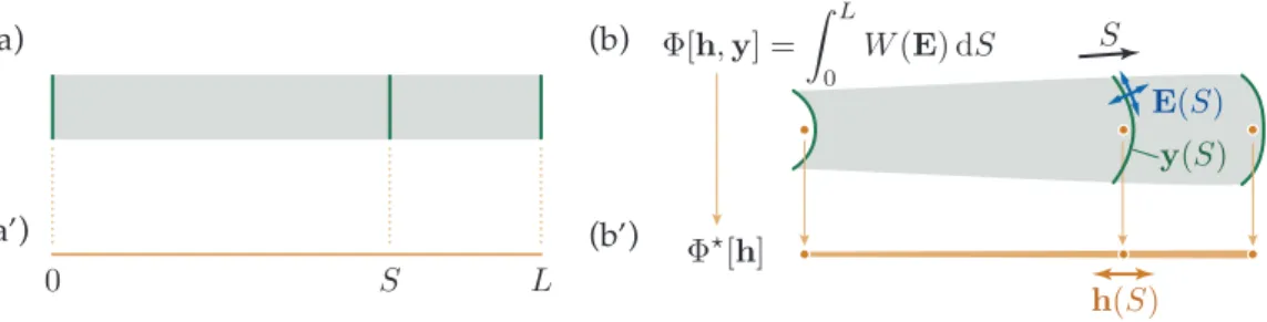
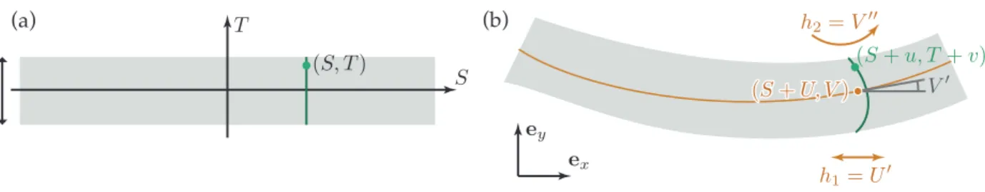
We assume that the structure is invariant along its longitudinal direction in the reference configuration, i.e., it is a block in two dimensions or a prismatic solid in three dimensions. The reference configuration does not need to be stress-free: naturally curved or twisted elastic rods for instance can be handled. The extension to structures whose geometric or mechanical properties are not invariant but slowly varying in the longitudinal direction is straightforward and will be discussed at the end of the paper. We denote by S a Lagrangian coordinate along the long dimension of the structure. The range of variation of S is denoted as 0 S L, where L typically denotes the natural length of the structure. The parameter S is used to label the cross-sections, see figure 1(a).
Let E(S) be the strain map over a particular cross-section S in the current configuration, as sketched in figure 1(b). By strain map, we mean that E(S) is the restriction to a particular cross-section of the set of strain measures relevant to the particular structural model. If we are dealing with a hyperelastic cylinder, for instance, E(S) collects all the strain components{ESS(·, ·), ESX(·, ·), EXX(·, ·), ESY(·, ·), EY Y(·, ·), EXY(·, ·)},
each taking the cross-section coordinates (X, Y ) as arguments.
Next, we introduce two mathematical objects in each cross-section: a vector of macroscopic strain h(S) = (h1(S), h2(S), . . .) made up of the strain measures that will survive in the 1d model, and a set of
microscopic degrees of freedom y(S) that will be ultimately be eliminated. Their exact definitions vary, but typically h(S) is the (apparent) 1d strain, as calculated from the center line passing through the centers
(a) (b)
(a’) (b’)
Figure 1: Dimension reduction for an abstract slender structure. Left column (a,a’): reference configuration highlighting a particular cross-section with coordinate S. Right-hand side column (b,b’): deformed configuration. Top row (a,b): full model used as a staring point, including a microscopic displacement y(S) and a microscopic strain E(S). Bottom row (a’,b’): equivalent 1d model obtained by dimension reduction, in which the details at the scale of cross-section are e↵ectively hidden.
of all the cross-section, while y(S) parameterizes the deformation of the cross-section relative to the center line. Typically, h(S) is a vector of low dimension, while y(S) is a (collection of) functions defined over the cross-sections, i.e., an infinite-dimensional vector. For the axisymmetric hyperelastic cylinder, for instance, h is made up of a single entry, the axial stretch, while y(S) is the cross-sectional map of displacement.
Together, the macroscopic strain h(S) and microscopic degrees of freedom y(S) determine the current configuration of the structure (up to a rigid-body motion) hence the microscopic strain E. Therefore, each particular structural model prescribes a method for calculating the cross-sectional strain map E(S) in terms of h, y and their longitudinal derivatives,
E(S) = E(h(S), h0(S); y(S), y0(S), y00(S)). (2.1) In the example of the cylinder, the longitudinal strain ESS depends on the longitudinal gradient of the
displacement, hence the dependence of E on y0.
Since y(S) is a function defined on the cross-sections, the function E in the right-hand side of (2.1) is a functional when the domain of the cross-section is continuous. Since E(S) is a map of strain over the cross-section, any dependence of the strain on the transverse gradients of displacement is hidden in the definition of E above. By contrast, we make sure that the dependence on longitudinal gradients takes place explicitly through the supplied argument y0 (and possibly y00). The additional dependence on y00 will allow
us to handle the bending of plates or shells without change. It is easy to take into account an additional dependence of E on higher-order gradients of h(S) or y(S); this does not a↵ect any of the results.
In terms of the strain map E(S), the structural model defines a density of strain energy W (E) per unit length dS. The strain energy of the structure therefore writes
[h, y] = Z L
0
W (E(h(S), h0(S); y(S), y0(S), y00(S))) dS, (2.2)
where the square brackets emphasize the functional dependence on the arguments.
Some structural models are conveniently expressed by imposing kinematic constraints q(y) = 0 on the microscopic displacement, where q(y) = (q1(y), q2(y), . . .). For structures whose cross-section involve
infinitely many degrees of freedom, y(S) is (a set of) functions defined in the cross-sections, i.e., q is a functional. We focus attention on kinematic constraints that are linear and independent of S. These assumptions can be relaxed easily. For structures that are free of kinematic constraints, we set q as the empty vector, q(y) = (), implying that any term such as q(y)· x = 0 must be discarded in the following.
We deal with dimension reduction by addressing the following relaxation problem: the macroscopic strain h(S) is prescribed and we seek the microscopic variables y(S) making the strain energy [h, y] stationary, subject to the kinematic constraint
8S q(y(S)) = 0. (2.3)
obtained by inserting the optimal microscopic displacement y(S) into , as in
?[h] = min
y:(8S)q(y(S))=0 [h, y]. (2.4)
This paper derives an expansion of ?[h] in successive derivatives of h(S) using an asymptotic method.
Note that the relaxed energy ?[h] is 1d: it no longer makes any reference to the cross-sectional degrees of
freedom. Once ?[h] has been obtained, the equilibrium equations for the 1d model can be derived using
standard variational techniques. 2.2. Analysis of homogeneous solutions
The first step in our analysis is to characterize homogeneous solutions under finite strain. To do so, we focus attention on the case where both the macroscopic strain h = (h1, h2, . . .) and the microscopic
displacement y are independent1of S. The strain for homogeneous solutions ˜E(h, y) is obtained by setting
h0= 0, y0= 0 and y00= 0 in (2.1) as
˜
E(h, y) = E(h, 0; y, 0, 0). (2.5) For a given value of the macroscopic strain h = (h1, h2, . . .), we seek the microscopic displacement y = yh=
y(h1,h2,...) such that the cross-sections are in equilibrium. To do so, we seek the value(s) of y that make
stationary the strain energy per unit length W ( ˜E(h, y)), among those satisfying the kinematic constraint q(y). This yields the variational problem
( 8ˆy dW dE( ˜E(h, yh))· ⇣ @ ˜E @y(h, yh)· ˆy ⌘ + fh· q(ˆy) = 0 q(yh) = 0, (2.6)
where the unknown fhis a Lagrange multiplier enforcing the constraint on the second line (fhcan be
inter-preted as the macroscopic load that is required for the homogeneous solution to be globally in equilibrium, such as a transverse external load in the case of a rod subject to a combination of uniform tension and bending). For structures whose cross-sections define a continuous domain in the plane, W (E) is a functional taking on scalar values, and dWdE(E)· E denotes the Gˆateaux derivative at E in the direction E. For structures possessing discrete cross-sectional degrees of freedom, dW
dE(E) the gradient of the function W (E).
Equation (2.6) warrants stationarity with respect to the microscopic displacement, but not with respect to the macroscopic strain. For a solution of these equations to represent an actual equilibrium, one would need to set up macroscopic forces conjugate to the macroscopic strain, labeled Fh in figure 2. If the
structure is an elastic cylinder, for instance, equation (2.6) imposes the contraction of cross-sections by Poisson’s e↵ect; to maintain the global equilibrium, a macroscopic tensile load, not discussed here, would be required. Macroscopic load do not enter into the dimension reduction process: they can be introduced directly in the 1d model, after the dimension reduction.
Equation (2.6) is a non-linear elasticity problem defined on the cross-section: the longitudinal variable has been removed. This problem can be solved, most often analytically (see the examples in the following sections) or in some cases numerically. By solving equation (2.6) for yh and fh for any value of the
macroscopic strain h, one obtains a catalog of homogeneous solutions, which is at the heart of the dimension reduction method. It is derived without any approximation: the catalog is made up of nonlinear solutions. In terms of the catalog of microscopic displacement yh, we can define the homogeneous strain Eh, the
homogeneous strain energy density Whom(h), the homogeneous pre-stress ⌃h, and the homogeneous tangent
sti↵ness, as follows, Eh = E(h, y˜ h) Whom(h) = W (Eh) ⌃h = dWdE(Eh) Kh = d 2W dE2(Eh). (2.7)
1Here, we are assuming that the splitting of the microscopic strain E(S) into master (h(S)) and slave (y(S)) degrees of
freedom has been set up in such a way that homogeneous solutions correspond to constant h and constant y. Any reasonable choice of h(S) and y(S) satisfies this property.
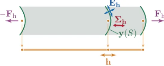
Figure 2: A homogeneous solution with uniform macroscopic strain h: microscopic displacement yh, microscopic strain Eh
and microscopic stress ⌃h. Note that the we are not interested at this stage in calculating the external loading Fh that
maintains equilibrium with respect to the macroscopic variables.
In our notation, the homogeneous quantities are either subscripted with the letters ‘hom’, as in Whom, or
simply by the vector of macroscopic strain h = (h1, h2, . . .) on which they depend.
2.3. Reduced models without gradient e↵ect
Most 1d models used for slender structures depend on macroscopic strain variables, but not on their gradients. The Euler-Bernoulli rod model, for instance, depends on curvature and twist and not on their gradients. These standard structural models are governed by the strain energy
?[h]
⇡ Z L
0
Whom(h(S)) dS (reduction without strain gradient),
and can therefore be derived directly from the catalog of homogeneous solutions. If we start from an elastic block, for example, and choose the axial strain and curvature as macroscopic variables, the strain energy R0LWhom(h(S)) dS defines a classical beam model (see §4.7). Note that the 1d model associated
with the energy functional ?[h] above might su↵er from poorer convexity properties than the original 3d
model; this happens typically when a string model is derived (i.e., when h(S) is set up to include just an axial strain variable, so that there is no bending energy in the resulting 1d model), and in this case an additional relaxation step is needed to remove the unphysical part of the constitutive law predicting axial compression (Acerbi et al., 1991).
So far, our method carries out dimension reduction without strain gradient. It does so without using any kinematic assumption and works under very general conditions: no material symmetry has been assumed, and it can handle inhomogeneous cross-sections and nonlinear elastic materials.
2.4. Microscopic correction, energy expansion
We return to the main focus of our work, which is on capturing strain-gradient e↵ects. Given a distribu-tion of macroscopic strain h(S) with 0 S L, we aim at calculating the optimal microscopic displacement y(S) and, thus, the relaxed energy ? appearing in equation (2.4). We do so by assuming slow variations
in the longitudinal direction: a proper stretched variable is introduced in the detailed proof of Appendix A, but it will suffice here to assume that the successive longitudinal derivatives of quantities such as h(S) scale like h =O(1), h0=O( ), h00=O( 2), etc., where
⌧ 1 is a slenderness parameter.
We seek the microscopic displacement y(S) that achieves the optimum in equation (2.4) in the form:
y(S) = yh(S)+ z(S). (2.8)
In words, we use the leading order microscopic displacement yh(S) obtained by looking up our catalog of
homogeneous solutions h7! yh as a first approximation; this look-up is performed with the parameter h set to the local prescribed value of the macroscopic strain, h = h(S). We refine this approximation by a correction z(S) proportional to the gradient term h0, which we calculate next.
To reflect the change of unknown from y(S) to z(S) in (2.8), let us first define the function eh that
yields the strain as in (2.1):
The variables bearing a dag (†) or a double dag (‡) are those that will be set later to the local value of the first or second gradients. The quantity h†, for instance, is a dummy variable that will be set later to h†= h0(S). Besides, ther in equation (2.9) stands for gradients with respect to the macroscopic strain h,
rky h=
dky h
dhk . (2.10)
Anticipating on the fact that we will need to expand the strain in (2.9), we define the structure coefficients eijklm(h) as the gradients of eh, evaluated at a homogeneous solution: for any set of integers (i, j, k, l, m),
eijklm(h) = @
(i+j+k+l+m)e h
[@h†]i[@h‡]j[@z]k[@z†]l[@z‡]m(0, 0; 0, 0, 0). (2.11)
Note that the upper set of indices correspond to gradients with respect to the gradients of the macroscopic strain parameters h† and h‡ while the lower set of indices correspond to gradients with respect to the microscopic variable z and its gradients z† and z‡. The quantities eij
klm(h) are either tensors, or operators
(if the cross-sectional degrees of freedom are continuous and at least one integer among k, l, m are non-zero): they will always appear contracted i times with h†, j times with h‡, k times with z, etc. Each one of these contractions will be denoted by a dot, representing either the standard contraction of tensors or the application of the operator.
The Taylor expansion of the strain (2.9) near a homogeneous solution can be written in terms of the structure coefficients as eh(h†, h‡; z, z†, z‡) = eh(0, 0; 0, 0, 0) + e10000(h)· h†+ e00100(h)· z + 1 2 ⇣ 2 h†· e10 100(h)· z + · · · ⌘ +· · · Structure coefficients will be calculated explicitly in the second part of the paper, when explicit structures are considered.
In terms of the structure coefficients, we further introduce the following operators, Ah· h† = ⌃h· (e10000(h)· h†) C(0)h · h‡ = ⌃h· (e01000(h)· h‡) C(1)h · z† = ⌃ h· (e00010(h)· z†) 1 2h†· B (0) h · h† = 1 2(e10000(h)· h†)· Kh· (e10000(h)· h†) +12⌃h· (h†· e20000(h)· h†) h†· rC (0) h · h† h†· B(1)h · z = (e10000(h)· h†)· Kh· (e00100(h)· z) + ⌃h· (h†· e10100(h)· z) h†· rC (1) h · z 1 2z· B (2) h · z = 1 2(e00100(h)· z) · Kh· (e00100(h)· z) +12⌃h· (z · e00200(h)· z). (2.12) They depend on the (local) macroscopic strain h. They operate on the cross-sectional degrees of freedom z and z† (but not z‡) and on the local values of the derivatives h† and h‡ of the macroscopic strain.
As shown in Appendix A, the expansion of the energy [h, yh+ z] in powers of the successive gradients
of macroscopic strain can be expressed in terms of these operators as
[h, yh+ z] = Z L 0 Whom(h(S)) dS + Z L 0 Ah(S)· h0(S) dS· · · + [C(0)h · h0+ C(1)h · z]LS=0+ Z L 0 ✓1 2h 0· B(0) h · h0+ h0· B (1) h · z + 1 2z· B (2) h · z ◆ S dS· · · +O(|h0|3,|h00||h0|2,|h000|). (2.13) In the boundary term in square brackets, both the arguments h in subscript of the operators and the operands h0 and z must be evaluated at S = 0 and S = L, respectively. Likewise in the integrand on the second line, the quantities h, h0 and z must be evaluated at the current point S.
The form of the strain gradient model above is similar to that derived in di↵erent contexts, see for example in Bardenhagen and Triantafyllidis (1994); our main contribution is a method for calculating the coefficients Ah(S), B(1)h , etc. explicitly.
2.5. Optimal correction
The last step in the reduction process is to determine the correction z(S) such that the microscopic displacement (2.8) satisfies the optimality condition (2.4). All derivatives of the unknown z(S) can be eliminated from equation (2.13), thanks to an integration by parts, as shown in Appendix A.5. The benefit is that the relaxation of the unknown z leads to a local problem in the cross-sections: as established in Appendix A, the optimal correction z(S) S is
z(S) = zopt(S) +O(|h0|2),
where the dominant contribution zopt = O(|h0|) is the one that minimizes the local elastic potential
z7!⇣1 2h0(S)· B (0) h(S)· h0(S) + h0(S)· B (1) h(S)· z + 1 2z· B (2) h(S)· z ⌘
, subject to the constraint q(z) = 0. The correction zopt(S) is therefore the solution to the following variational problem,
( 8ˆz h0(S)· B(1)h(S)· ˆz + zopt(S)· B (2) h(S)· ˆz fopt(S)· q(ˆz) = 0 q (zopt(S)) = 0, (2.14)
where fopt(S) is a Lagrange multiplier, to be determined as part of the solution process.
This variational problem is linear with respect to the local value of the strain gradient h0(S). This implies that its solution zopt(S) is proportional to h0(S), i.e., there exists a catalog of corrections Zh(S)opt such that
zopt(S) = Zh(S)opt · h0(S). (2.15)
The catalog Zhoptis found by solving (2.14). It can be determined once for all in terms of the geometric and
mechanical properties of a reference cross-section and in terms of the macroscopic strain h, as we show in the examples.
Equation (2.14) is a problem of linear elasticity in the cross-section. The first term h0(S)· B(1)h(S)· ˆz can be interpreted as a pre-stress arising from the presence a gradient (an interpretation of this pre-stress term will be obtained based on the analysis of specific structures, see§5.4 in particular). The second term zopt(S)· B(2)h(S)· ˆz is an elastic sti↵ness term which, in view of the definition of B(2)h(S) in equation (2.12)
has two contributions: a tangent elastic sti↵ness Kh(S), and a geometric sti↵ness arising from the pre-stress
⌃h(S) associated with the local state of stress.
2.6. Relaxed energy
The relaxed energy ?[h] is finally obtained by inserting the optimal displacement y(S) = y h(S) +
zopt(S) +· · · into the energy expansion in equation (2.13). The result is
?[h] =Z L 0 Whom(h(S)) dS + Z L 0 Ah(S)· h0(S) dS + [Ch(S)· h0(S)]L0 + 1 2 Z L 0 h0(S)· Bh(S)· h0(S) dS + . . . (2.16) Here, the operator Ahhas been introduced in equation (2.12) and the additional elastic moduli Bhand Ch
are defined by Bh = B(0)h ⇣ Zhopt ⌘T · B(2)h · Z h opt, Ch = C(0)h + C (1) h · Z h opt. (2.17)
The energy functional in equation (2.16) and the explicit expression for the strain-gradient modulus Bh
are the main results of this paper.
In equation (2.16), the leading order term in the expansion depends Whom, and defines structural models
without the gradient e↵ect, see§ 2.3. The second term depending on Ahyields an energy contribution that
(a) (b)
Figure 3: An axisymmetric membrane: (a) reference and (b) current configurations.
forthcoming examples. The terms depending on Chis a boundary term arising from a gradient e↵ect, while
the last term is the bulk strain-gradient term.
For further reference, we note that the strain gradient term is available in alternative form as
1 2 Z L 0 h0(S)· Bh(S)· h0(S) dS = 1 2 Z L 0 h0(S)· B(0)h(S)· h0(S) dS 1 2 Z L 0 zopt· B(2)h · zoptdS.
2.7. A necessary stability condition at the microscopic scale
A necessary condition for the microscopic correction derived in section 2.5 to be stable (and, hence, for the relaxed energy ? to be meaningful) is that the sti↵ness operator B(2)
h appearing in the microscopic
problem in equation (2.14) is non-negative,
(8z such that q(z) = 0) z · B(2)h · z 0. (2.18)
Note that this condition does not warrant that the matrix Bhof strain-gradient moduli is non-negative, see
equation (2.17) (a matrix Bh having negative eigenvalues is indeed obtained for the elastic block, see§4.7).
However, equation (2.18) does warrant 1 2h 0(S)· B h(S)· h0(S) 1 2h 0(S)· B(0) h · h0(S),
which, as discussed in section 6, shows that our 1d model relaxes the elastic energy better than strain gradient models derived from the ad hoc kinematic assumption z(S) = 0: this benefit is a consequence of the fact that our 1d model is asymptotically exact.
3. Application to an axisymmetric membrane
Upon inflation, axisymmetric rubber membranes feature localized deformations in the form of propa-gating bulges (Kyriakides and Chang, 1991). Standard dimension reduction without gradient terms yields a non-convex elastic potential Whom and thus fails at describing the details of localization. Localized
so-lutions can be analyzed using the full membrane model (Fu et al., 2008; Pearce and Fu, 2010), but are more easily and very accurately described based on a 1d strain-gradient model, as recently shown by the authors, starting from the theory of axisymmetric elastic membranes and using a typical constitutive law for rubber (Lestringant and Audoly, 2018). This 1d model is rederived here as a first illustration of the general reduction method presented in section 2.
3.1. Full axisymmetric membrane model
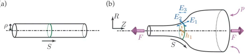
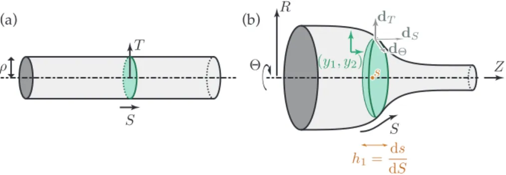
The reference configuration is chosen as the natural, cylindrical configuration of the membrane, and the natural radius of the circular membrane is denoted by ⇢. In the current configuration, the membrane is deformed under the action of an inflating pressure p, and a pulling force F equally distributed over the terminal cross-sections, see figure 3. Natural boundary conditions are used, i.e., there is no restraint on the terminal cross-sections.
An axisymmetric configuration of the membrane is parameterized by two functions Z(S) and R(S), such that the cross-section with arc-length coordinate S in the reference configuration is transformed into a circle perpendicular to the axis of the shell, with axial coordinate Z(S) and radius R(S), see figure 3(b). We consider a standard set of strain measures from the theory of finite-strain axisymmetric elasticity, E = ⇣ pZ02+ R02 R
⇢ Z0
⌘
: E1 = pZ02+ R02 and E2 = R⇢, usually denoted as (E1, E2) = ( S, ⇥),
are the membrane stretches in the (principal) longitudinal and circumferential directions, respectively. The additional ‘strain’ E3has been included for convenience, as it allows us to write the potential energy of the
pulling force F as F [Z(S)]L 0 = F
RL 0 E3dS.
The sum of the membrane strain energy, and the potential energy of the loads p and F is captured by an e↵ective potential W (E) per unit length dS,
W (E) = W (E1, E2) p ⇡ ⇢2E22E3 F E3,
where W (E1, E2) = W ( S, ⇥) is the strain energy of the hyperelastic membrane model (we use bars
generally for quantities relating to the full model). Upon integration with respect to S, the second term yields ( p) times the volume enclosed by the membrane, which is the potential energy of the pressure force. Note that we have chosen to include the potential energy of the loads p and F into the potential =R0LW dS which normally captures the strain energy only; in line with this, the loading parameters p and F are considered constant.
3.2. Macroscopic and microscopic variables
A natural choice of macroscopic strain parameter is the apparent axial stretch Z0(S): this is the stretch of a virtual bar obtained by collapsing all the circular cross-sections to a point located at their center. However, this choice has the drawback that, for typical constitutive laws for rubber, there can be several homogeneous solutions corresponding to a given value of the apparent stretch. To work around this difficulty, it is preferable to define instead the macroscopic strain parameter as the hoop stretch h1(S) = E2(S) = R(S)⇢ .
As we will see, it is possible to reconstruct the apparent axial stretch Z0(S) in terms of this h
1(S). We thus
apply the general formalism using a single macroscopic strain and a single microscopic degree of freedom, defined as h(S) = (h1(S)) = ✓R(S) ⇢ ◆ , y(S) = (y1(S)) = (Z0(S)).
With this choice of macroscopic and microscopic variables, it is possible to reconstruct the configuration using R(S) = ⇢ h1(S) and Z(S) = Z(0) +R
S
0 y1(S) dS, where Z(0) is an unimportant rigid-body translation.
As we do not need any constraint for this particular structural model, we set q(y) = () and drop all the terms containing q(y) in the general formalism.
The strain vector E for the axisymmetric membrane given in section 3.1 can be cast in the canonical form from equation (2.1) by choosing the strain function as
E(h, h†; y, y†, y‡) =⇣ q⇢2h†2
1 + y21 h1 y1
⌘ ,
where the arguments are vectors whose length matches that of the macroscopic strain h and microscopic variable y proposed above, i.e., h = (h1), h†= (h†1), y = (y1), y† = (y1†) and y‡ = (y‡1).
3.3. Homogeneous solutions
Homogeneous solutions are first analyzed, by setting to zero the derivative terms in the definition of the strain, see equation (2.5). This yields the homogeneous strain as
˜
E(h, y) = y1 h1 y1 .
The generalized stress in the homogeneous solution is given by the gradient of the potential E(S), dW
dE( ˜E(h, y)) = ⌃S(y1, h1) ⌃⇥(y1, h1) 2 p ⇡ ⇢
2h
where ⌃S( S, ⇥) = @@WS( S, ⇥) and ⌃⇥( S, ⇥) = @@W⇥( S, ⇥) are the components of the Piola-Kirchho↵
stress in the longitudinal and circumferential directions, respectively, as predicted by the elastic strain potential W ( S, ⇥) characterizing the elastic properties of the membrane.
Next, we proceed to write and solve the principle of virtual work (2.6) for homogeneous solutions. Noting that @ ˜@yE(h, y) = 1 0 1 , it writes
⌃S(y1(h1), h1) + F + p ⇡ ⇢2h21= 0. (3.1)
This is an equation for the longitudinal stretch y(h1)
1 in a homogeneous solution, in terms of the hoop stretch
h1 = R⇢. The load parameters F and ⇢ are considered fixed, i.e., the dependence on F and ⇢ will always
be silent. Equation (3.1) expresses the equilibrium of a homogeneous solution in the longitudinal direction. For typical constitutive laws, equation (3.1) cannot be solved explicitly for y(h1)
1 in terms of h1, and will be
viewed as an implicit equation.
In terms of the homogeneous solution y(h1)
1 , we obtain the properties of homogeneous solution from
equation (2.7) as E(h1) = ⇣ y(h1) 1 h1 y1(h1) ⌘ Whom(h1) = W (y(h1 1), h1) ⌃S(y1(h1), h1) y1(h1) ⌃(h1) = ⇣ ⌃S(y(h1 1), h1) ⇤ ⌃S(y1(h1), h1) ⌘ K(h1) = 0 @ KSS(y (h1) 1 , h1) ⇤ 0 ⇤ ⇤ ⇤ 0 ⇤ 0 1 A . (3.2)
Here, the star symbol (⇤) denote quantities that play no role and do not need to be calculated. The quantity KSS( S, ⇥) = @
2W
(@ S)2( S, ⇥) is the tangent elastic modulus, as calculated from the membrane model.
3.4. Change of microscopic variable
According to the general method, we introduce a correction z(S) = (z1(S)) to the microscopic variable
by y(S) = yh(S) + z(S), i.e., y1(S) = y1(h1(S))+ z1(S). In terms of the new unknown, the strain function
reads, see equation (2.9),
eh(h†, h‡; z, z†, z‡) = ⇣ q ⇢2h†2 1 + (y (h1) 1 + z1)2 h1 y1(h1)+ z1 ⌘ ,
where again the arguments are vectors whose dimension is imposed by the macroscopic strain and microscopic variable as h† = (h†1), h‡= (h‡1), z = (z1), z† = (z1†) and z‡= (z‡1). Note that the strain function eh= e(h1)
depends on the macroscopic strain h1which appears in subscript, and that we have made use of the catalog
of homogeneous solutions y(h1)
1 in the right-hand side.
The structure coefficients eijklm(h) are the successive partial derivatives of the right-hand side above, see equation (2.11). These partial derivatives are most easily found by identifying eh(h†, h‡; z, z†, z‡) with its
Taylor expansion ✓ y(h1) 1 + z1+ ⇢ 2h†2 1 2 y1(h1) h1 y1(h1)+ z1 ◆ . The result is e10 000(h) = 0 e20000(h) = ⇣ ⇢2 y(h1)1 0 0 ⌘ e01 000(h) = 0 e10100(h) = 0 e00100(h) = 1 0 1 e00200(h) = 0 e00010(h) = 0. (3.3)
These are the only structure coefficients that are required in the following. Recall that the dimension of both h and y is one for an axisymmetric membrane: the tensors eijklm, which are of dimensions 3⇥1⇥· · ·⇥1 according to the general rule, where the one’s are repeated i + j + k + l + m times, have been identified with vectors of dimension 3.
When these expressions are combined with those for homogeneous quantities obtained in (3.2), one can calculate the first batch of operators from equation (2.12) as
Ah· h† = ⌃h· (e10000(h)· h†) = ⌃h· 0 = 0 C(0)h · h‡ = ⌃h· (e01000(h)· h‡) = ⌃h· 0 = 0 C(1)h · z† = ⌃ h· (e00010(h)· z†) = ⌃h· 0 = 0 1 2h†· B (0) h · h† = 120· Kh· 0 + 1 2⌃h· ⇣ ⇢2 y(h1)1 (h†1)2 0 0 ⌘ h†· 0 · h†= 1 2⌃S(y (h1) 1 , h1) ⇢ 2 y1(h1)(h † 1)2 h†· B(1)h · z = 0 · Kh· (⇤) + ⌃h· 0 h†· 0 · z = 0 1 2z· B (2) h · z = 1 2 1 0 1 · Kh· 1 0 1 + 1 2⌃h· 0 = 1 2KSS(y (h1) 1 , h1) (z1)2.
3.5. Local optimization problem
The local optimization problem (2.14) is particularly simple, because it has no source term (B(1)h = 0) and no constraint term (q(y) = ()). In view of the operators just derived, it reads
8ˆz1 zˆ1KSS(y1(h1), h1) z1opt= 0.
We rule out the possibility of a material instability in the membrane model, i.e., KSS(y1(h1), h1) > 0 (note that
with this assumption of material stability at the ‘microscopic’ level, the stability condition from section 2.7 is automatically satisfied). The variational problem above can then be solved for zopt= zopt1 as zopt( ˜S) = 0.
The correction to the microscopic variable arising from the gradient e↵ect is zero for this particular structure. To comply with the general form of equation (2.15), we set accordingly Zhopt= 0 .
3.6. Regularized model
In view of equation (2.17), we obtain the operators entering into the strain-gradient model as Ah= 0,
Bh= (B11(h1)) where B (h1) 11 = ⇢2⌃ S(y1(h1),h1) y(h1)1 and Ch= 0.
We switch to the more standard notation ⇥ = h1 = R⇢ for the hoop stretch and S = y1 for the
apparent axial stretch, and recapitulate the main results for the axisymmetric membrane as follows. We must first solve the implicit equation (3.1) for the apparent axial stretch y(h1)
1 = homS ( ⇥), which reads
⌃S homS ( ⇥), ⇥ = F + p ⇡ ⇢2 2⇥ and yields the homogeneous equilibria of the balloon. In this equation,
⌃⇥( S, ⇥) = @@W⇥( S, ⇥) is the hoop stress in the homogeneous solution. In terms of this catalog of
homogeneous solutions, we can calculate Whom( ⇥) by (3.2). The balloon is governed by the strain-gradient
bar model, see equation (2.16),
?[ ⇥]⇡ Z L 0 Whom( ⇥(S)) + 1 2B( ⇥(S)) 02 ⇥(S) dS, (3.4a)
where the strain-gradient modulus reads
B( ⇥) = ⇢2⌃ S homS ( ⇥), ⇥ hom S , (3.4b)
and where ⌃S( S, ⇥) =@@WS( S, ⇥) is the longitudinal stress in the homogeneous solution.
3.7. Comments
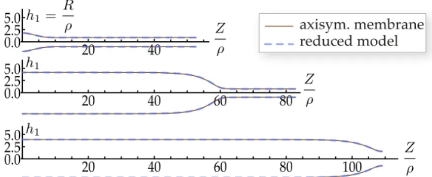
We have recovered the model established by Lestringant and Audoly (2018). Typical solutions predicted by the 1d model are compared to those of the full axisymmetric model in figure 4: the 1d models appears to be highly accurate, even in the regime where the bulges are fully localized.
The axisymmetric membrane model, which we used as a starting point was already a 1d model: it does not make use of any transverse variable, and has discrete degrees of freedom (Z, R) in each cross-section. The
axisym. membrane reduced model 20 2.5 5.0 40 60 80 100 20 2.5 5.0 40 60 80 20 2.5 0.0 0.0 0.0 5.0 40
Figure 4: Solutions for a propagating bulge in an axisymmetric membrane with initial aspect ratio L/⇢ = 30: comparison of the predictions of the full axisymmetric membrane model (§3.1) and of the reduced model in equation (3.4), from Lestringant and Audoly (2018). The material model for rubber proposed by Ogden (1972) is used, with the same set of material parameters as used in the previous experimental work of Kyriakides and Chang (1991), see also§2 in Lestringant and Audoly (2018).
reduction method led us to another 1d model and it therefore is improper to speak of dimension reduction in this case. The reduction method is still useful, as reduced model is simpler and, more importantly, much more standard: it is the well-known di↵use-interface model introduced by van der Walls in the context of liquid-vapor phase transition, as discussed by by Lestringant and Audoly (2018).
Even when bulges are fully formed, the typical length of the interface between the bulged and unbulged regions never gets much less than⇠ ⇢, i.e., remains always much larger than than the membrane’s thickness t (assuming the membrane is thin in a first place ⇢ t). This warrants that the assumptions underlying the membrane model remain valid. To address the case of thick membranes, i.e., when the ratio t/⇢ is not small, one could apply our reduction method to a theory of thick membranes, or to a finite-strain model for a hyperelastic cylinder in 3d.
4. Application to a linearly elastic block
Our next example is a homogeneous block of linearly elastic material in 2d, having length L and thickness a, as sketched in figure 5. We account for both stretching and bending of the block. In the first step of the dimension reduction, we will recover the classical beam model. Its energy is convex, implying that this particular structure does not tend to localize. The strain-gradient model obtained at the next step is still of interest as its solutions generally2converge faster towards those of the full (2d) elasticity model than those
of the classical beam model.
There is a large amount of work on higher-order asymptotic expansions for prismatic solids in the specific context of linear elasticity with the aim to derive linear higher-order beam theories, see for instance the work of Trabucho and Via˜no (1996). The forthcoming analysis shows that these results can be easily recovered with our method. It also reveals that the assumption of linear elasticity brings in severe, somewhat hidden limitations.
The elastic block is our first example where a cross-section possesses infinitely many degrees of freedom.
4.1. Full model: a linearly elastic block in 2d
We consider an elastic block in reference configuration. The axial and transverse coordinates in reference configuration are denoted as S and T , respectively, and are used as Lagrangian coordinates. Their domains are 0 S L and a/2 T a/2.
2It is known, however, that boundary conditions can prevent strain-gradient models from converging faster. This happens
when the imposed boundary conditions are incompatible with the kinematics y(S) = yhom(h(S)) + zopt+· · · of the
strain-gradient model at the microscopic scale. We do not address this question in this paper, and limit attention to natural boundary conditions.
(a) (b)
Figure 5: A block of a linearly elastic material in (a) reference and (b) current configuration. The 1d model makes use of the center line (brown curve), defined as the curve passing through the centers of mass (brown dots) of the cross-section. The macroscopic strain are the apparent stretch h1(S) = U0(S) and the apparent curvature h2(S) = V00(S) of the center line.
We introduce the displacement (u, v) in a Cartesian frame (ex, ey) aligned with axes of the undeformed
block: a point with position (S, T ) in reference configuration gets mapped to x(S, T ) = (S + u(S, T ), T + v(S, T )) in the current configuration, see figure 5(b). The linear strain is presented in vector form as
E = @u @S @v @T 1 2 @u @T + @v @S (4.1)
where E1, E2 and E3 are respectively the SS, T T and ST components of the 2-d strain tensor from linear
elastic theory. We use a linear isotropic and uniform constitutive in 2d (Hookean elasticity), corresponding to an elastic potential per unit length dS
W (E) = 1 2 Z +a/2 a+2 (2 µ (E2 1+ E22+ 2 E23) + (E1+ E2)2) dT, (4.2)
where the elastic constants µ and are known as the Lam´e parameters.
4.2. Macroscopic and microscopic variables
We choose to define the center line as the curve passing through the centers of mass of the cross-sections. The components of the center line displacement are therefore
U (S) =hui(S) V (S) = hvi(S), (4.3) wherehfi(S) = 1
a
R+a/2
a/2f (S, T ) dT denotes the cross-section average of a function f (S, T ).
The deformed center line is parametrized as (S + U (S)) ex+ V (S) ey. In the theory of linear elasticity,
it is associated with an apparent longitudinal strain U0(S), deflection angle V0(S), and curvature V00(S),
where by ‘apparent’ we emphasize the fact that the center line is non-material. In our reduction of the elastic block to a 1d model, we use as macroscopic strain measures these apparent axial strain and curvature,
h(S) = (U0(S), V00(S)).
Let ˜x(S, T ) the final position of the point initially at position S ex+ T ey if the cross-section S were to
undergo a rigid body motion following the center line, namely the combination of a rigid-body translation (U (S) ex+V (S) ey) and a rigid-body rotation with angle V0(S). Since V0(S) is infinitesimal, the unit normal
to the center line writes V0(S) ex+ ey and so ˜x(S, T ) = [(S + U (S)) ex+ V (S) ey] + T [ V0(S) ex+ ey].
We choose to define the microscopic displacement y(S, T ) as the di↵erence between the actual position x(S, T ) = (S + u(S, T )) ex+ (T + v(S, T )) ey and ˜x(S, T ):
y(S, T ) = x(S, T ) x(S, T ) = (u(S, T )˜ U (S) + V0(S) T ) ex (v(S, T ) V (S)) ey.
The Cartesian components are found as y1(S, T ) = u(S, T ) U (S) + V0(S) T and y2(S, T ) = v(S, T ) V (S).
This definition of y warrants y(S, T ) = 0 automatically whenever the block is moved rigidly, since x(S, T ) = ˜
In our general presentation of the method in section 2, y(S) (with a single argument) was defined as the collection of the microscopic degrees of freedom on a given cross-section S. To comply with this convention, we define y(S) = (y1(S), y2(S)) as a pair of functions defined on the cross-section taking the transverse
coordinate T as an argument,
y1(S) = {(u(S, T ) U (S) + V0(S) T )}T
y2(S) = {v(S, T ) V (S)}T.
We recall that {g(T )}T is a notation for the function g that maps T to g(T ), the index T appearing in
subscript after a curly brace being a dummy variable.
In view of equation (4.3), the microscopic displacement must satisfy the condition hui(S) = U(S) and hvi(S) = V (S). Upon elimination of (u, v) in favor of (y1, y2), this yields hy1(S)i = hy2(S)i = 0 for all S.
We handle these constraints by setting
q(y) = 1 a Z a/2 a/2 y1(T ) dT, Z a/2 a/2 y2(T ) dT !
in the general formalism of section 2.
The displacement in the Cartesian basis is u(S, T ) = U (S) + [y1(S)](T ) V0(S) T and v(S, T ) =
[y2(S)](T ) + V (S), and therefore the strain in equation (4.1) can be expressed as
E(S) = h1(S) + [y10(S)](T ) h2(S) T @T[y2(S)](T ) 12(@T[y1(S)](T ) + [y02(S)](T )) .
Since primes are reserved for derivatives with respect to the longitudinal variable S, we use the symbol @T
for transverse derivatives. In the above expression, y0
1(S) denotes the function {y10(S, T )}T, and similarly y20(S) = {y20(S, T )}T.
For consistency with the discrete case, we define the strain function E(. . .) as an operator that takes as arguments the pair of functions y = y(S) = (y1(S), y2(S)), and their derivatives y† = y0(S), as well as the
pair of scalars h(S) = (h1(S), h2(S)), and returns the strain map in the cross-section,
E(h, h†, y, y†, y‡) =⇣ {h1+ y†1(T ) h2T}T {@Ty2(T )}T n 1 2(@Ty1(T ) + y † 2(T )) o T ⌘ . (4.4)
We use the same ordering conventions for the strain components as in equation (4.1), i.e. the longitudinal, transverse and shear strain appear in this order. We continue to use the same notation as earlier whereby variables bearing a dagger, such as h† = (h†1, h†2) are dummy variables that are intended to hold the local value of the derivative, here h0(S).
4.3. Homogeneous solutions
In the homogeneous case, the arguments of E corresponding to axial gradients in (4.4) (thus, bearing a single or a double dagger) are all set to zero, see equation (2.5). Doing so, we are left with the map of homogeneous strain,
˜
E(h, y) = {h1 h2T}T {@Ty2(T )}T 12@Ty1(T ) T .
The first variation of the strain energy (4.2) is calculated as
W = dW dE( ˜Eh)· E = Z +a/2 a+2 ⇤ E1+ (2 µ + ) E2 4 µ E3 · E(T ) dT = Z +a/2 a+2 ⇤ (h1 h2T ) + (2 µ + ) @Ty2 2 µ @Ty1 · E(T ) dT,
By setting the variation of strain as E = @ ˜E(h,y)@y · ˆy = {0}T {@Tyˆ2}T 12@Tyˆ1 T as in
equa-tion (2.6), we obtain the principle of virtual work as
8(ˆy1, ˆy2) Z +a/2 a/2 ✓ (2 µ @Ty1)1 2@Tyˆ1+ f h 1 yˆ1 ◆ dT + Z +a/2 a/2 ( ( (h1 h2T )+(2 µ+ ) @Ty2) @Tyˆ2+f2hyˆ2) dT = 0 where fh= (fh 1, f2h) is a Lagrange multiplier.
The solution satisfying the constraint q(y) = 0 is found as yh 1 = {0}T yh 2 = n ⌫ h1T + ⌫ h2 ⇣ T2 2 a2 24 ⌘o T fh = 0
where we have defined the 2-d Poisson’s ratio ⌫ = 2 µ+ . We also define the Young’s modulus in 2d as Y =4 µ ( +µ)2 µ+ (note that these expressions of ⌫ and Y are valid for 2d elasticity but not for 3d elasticity).
We can then calculate the quantities characterizing the homogeneous solutions from equation (3.2) as Eh = {h1 h2T}T { ⌫ (h1 h2T )}T {0}T
Whom(h) = 12(Y a h21+ Y I h22)
⌃h· E = R+a/2a+2 Y (h1 h2T ) 0 0 · E(T ) dT
E· Kh· E = R+a/2a+2 E(T )·
0 @ ⇤⇤ 2 µ +⇤ 00 0 0 4 µ 1 A · E(T ) dT, (4.5)
where I =R+a/2a/2 T2dT =a3
12 is the geometric moment of inertia of the cross-section.
4.4. Change of microscopic variable
Seeking the microscopic displacement as y(S) = yh(S) + z(S) from equation (2.8), we can calculate the
strain in terms of the new microscopic variable z as
eh(h†, h‡; z, z†, z‡) = ⇣ {h1+ z†1(T ) h2T}T { ⌫ (h1 h2T ) + @Tz2}T . . . n 1 2 ⇣ ⌫ h†1T + ⌫ h†2 ⇣ T2 2 a2 24 ⌘ + @Tz1+ z2† ⌘o T ⌘ .
where h = (h1, h2), h† = (h†1, h†2), z = ({z1(T )}T,{z2(T )}T) and z† = ({z†1(T )}T,{z2†(T )}T). For the linear
elastic block, the structure coefficients do not depend on h‡ or z‡.
The structure coefficients introduced in equation (2.11) are then obtained as e10 000(h)· h† = ⇣ 0 0 n ⌫2 ⇣h†1T h†2 ⇣ T2 2 a2 24 ⌘⌘o T ⌘ e20 000(h) = 0 e01000(h) = 0 h†· e10100(h)· z = 0 e00100(h)· z = 0 {@Tz2}T 12@Tz1 T z· e00 200(h)· z = 0 e00010(h)· z†= ⇣ {z1†}T 0 n 1 2z † 2 o T ⌘ . Next, the operators introduced in (2.12) are calculated as follows,
Ah = 0 C(0)h = 0 C(1)h · z = R+a/2a+2Y (h1 h2T ) z1dT 1 2h†· B (0) h · h† = 1 2 R+a/2 a+2µ ⌫ 2 ⇣h† 1T h†2 2 ⇣ T2 a2 12 ⌘⌘2 dT = 1 2µ ⌫ 2 ⇣a3 12h † 1 2 + a5 720h † 2 2⌘ h†· B(1)h · z = ⌫ µR+a/2a+2⇣h†1T h†2 2 ⇣ T2 a2 12 ⌘⌘ @Tz1dT Y R +a/2 a+2(h † 1 h†2T ) z1dT 1 2z· B (2) h · z = 1 2 R+a/2 a+2(2 µ + ) (@Tz2) 2+ µ (@ Tz1)2dT. (4.6)
4.5. Local optimization problem The correction zopt = zopt1 , z
opt
2 to the cross-sectional displacement is found by writing down the
variational problem (2.14), 8(ˆz1(T ), ˆz2(T )) Z +a/2 a+2 µ ✓ @Tz1[1] ⌫ ✓ h02 T2 2 + h 0 1T + h02 a2 24 ◆◆ @Tˆz1 Y (h01 h02T ) ˆz1 dT . . . + Z +a/2 a+2 ⇥ (2 µ + ) @Tz2opt@Tzˆ2⇤dT 1 a Z +a/2 a/2 f1optzˆ1+ f2optzˆ2 dT = 0.
We proceed to solve this variational problem together with the incremental constraint⌦z1opt↵=⌦zopt2 ↵= 0. As there is no source term in factor of ˆz2, the transverse solution is easily found as z2opt(T ) = 0 and f
opt 2 = 0.
The remaining terms in the variational problem above concern the axial correction, and can be rearranged as 8ˆz1(T ) Z +a/2 a+2 f1opt a + Y h 0 1 ! Y h02T ! ˆ z1 µ ✓ @Tzopt1 ⌫ ✓ h02 T2 2 + h 0 1T + h02 a2 24 ◆◆ @Tzˆ1dT = 0.
The solution to this equation satisfying the constraint⌦z1opt
↵
= 0 can be worked out as
f1opt = a h01Y z1opt(T ) = h01⌫ 2 ⇣ T2 a2 12 ⌘ h0 2 24((6 + 5 ⌫) a 2T 4 (2 + ⌫) T3).
The detailed expression of z1opt will not be used, other than to evaluate the following integral,
Z a/2 a/2 @Tzopt1 2 dT = a 3⌫2 12 h 0 1 2 + ✓ 1 30+ 11 ⌫ 180 + 7 ⌫2 240 ◆ a5h02 2 .
To sum up, the displacement correction zopt = z1opt, z opt
2 can be written in terms of a fixed basis of
functions as zopt = Zhopt· h0, where
Zhopt= ⌫ 2 ⇣ T2 a122⌘ 241 ((6 + 5 ⌫) a2T 4 (2 + ⌫) T3) 0 0 ! .
The entries in the top-left (respectively top-right) slot is a longitudinal displacement along ex in response
to a gradient of axial strain h1= U0 (respectively, to a gradient of curvature h2= V00).
The necessary stability condition from section 2.7 requires 2 µ + 0 and µ 0, which are standard condition of material stability in 2d, as discussed for example in Barenblatt and Joseph (1997).
4.6. Regularized model
Two last operators are defined in equation(2.17). They can now be evaluated as
h†· Bh· h†= µ ⌫2 ✓a3 12h † 1 2 + a 5 720h † 2 2◆ µ Z +a/2 a+2 (@Tz1)2dT = µ a5 ✓ 1 30+ 11 ⌫ 180 + ⌫2 36 ◆ h†22= Y a56 + 5 ⌫ 360 h † 2 2 (4.7) and Ch· h†= Z +a/2 a+2 Y (h1 h2T ) ⌫ 2 ⇣ T2 a2 12 ⌘ 1 24((6 + 5 ⌫) a 2T 4 (2 + ⌫) T3) ! · h†dT = Y a512 + 11 ⌫ 720 h2h † 2.
In addition, recall that Ah= 0.
Using equation (2.16), we obtain the energy function of the 1d model as
?[h] =Z L 0 1 2(Y a h 2 1+ Y I h22) dS + Y a5 12 + 11 ⌫ 720 [h2h 0 2]L0 1 2Y a 56 + 5 ⌫ 360 Z L 0 h022 dS, (4.8)
where h1= U0 denotes the axial stretch and h2= V00 denotes the curvature.
4.7. Comments
We have recovered the classical Euler-Bernoulli rod model at the dominant order, with a stretching modulus Y a and a bending modulus Y I. Indeed, the first step of the reduction method yields classical structural model (i.e., without the gradient e↵ect), see the expression of Whom in equation (4.5).
As the operator 12z· B(2)h · z in equation (4.6) is non-negative, the necessary condition of stability with
respect to the microscopic degrees of freedom is satisfied, see§2.7. However, the coefficient of the gradient term h02
2 in (4.8) is negative, like the second-gradient modulus Bh acting on the macroscopic degrees of
freedom, see (4.7). As a result, ?[h] can be decreased without bound by means of small-scale oscillations.
This behavior can likely be regularized by pushing the expansion to a higher order. In its present form, the functional (4.8) should not be used to set up a minimization or to analyze stability; it is still useful, as its stationary points provide a more accurate approximation of the 3d solution than that of the Euler-Bernoulli model.
To connect with the existing literature, we have worked out this example in the limited context of linear elasticity but the derivation can be extended easily to deal, e.g., with a nonlinear constitutive law, a nonlinear geometry, as demonstrated in the following section. While previous work has been focused on deriving order by order solutions to the 3d equilibrium equations, our relaxation method makes use of the variational structure of these equations by working directly on the energy. This, together with the fact that the hard work underlying the derivation of the general method in section 2 and Appendix A has been done once for all, simplifies the reduction of any particular structural model considerably.
The only gradient e↵ect present in equation (4.8) comes from the gradient of bending. The absence of a gradient term for stretching is a peculiarity of the linear elasticity model which we started from: a gradient e↵ect involving the axial strain h1 is restored if we start instead from a finite-elasticity theory, as
the next example will show. In fact, it does not make much sense to derive a higher-order rod model , which aims at identifying subdominant corrections to the elastic energy, starting from a linear elasticity model : the linearization underlying the linear elasticity theory suppresses subdominant contributions to the strain energy a priori. This fact has not been well appreciated, as most of the earlier work on higher-order beam models has been done in the framework of linear elasticity.
5. Application to a hyperelastic cylinder in tension
In our third example, we address the axisymmetric deformation of a hyperelastic cylinder. This problem is motivated by the necking of bars, a situation where deformations become localized. Necking typically involves plasticity but it can be analyzed using an equivalent elastic constitutive law obtained by the J2
deformation theory, as long as the loading is proportional and monotonous: the equivalent hyperelastic law is such that the curve for homogeneous traction displays a maximum of the force as a function of the stretch, leading to localization. This section derives the 1d model obtained by Audoly and Hutchinson (2016) using a dedicated expansion method, this time using the general method of section 2. This worked example combines a continuous cross-section, a nonlinear elastic model, and kinematic constraints.
5.1. Finite-strain elasticity model for an axisymmetric bar
In its reference configuration, the bar is a cylinder with length L and radius ⇢, and we denote by S, T and ⇥ the axial, radial and azimuthal coordinates, respectively, with 0 S L, 0 T ⇢, 0 ⇥ 2 ⇡. We consider a transversely isotropic material whose elastic properties are functions of T but not of ⇥ or
(a) (b)
Figure 6: A nonlinearly elastic cylinder in (a) reference configuration and (b) current configuration.
S (isotropy is a particular case of transverse isotropy, so this includes homogeneous isotropic materials): this warrants that axisymmetric solutions possessing cylindrical invariance exist when the bar is subject to traction. In fact, we restrict attention to axisymmetric solutions, ignoring the possibility of localized modes involving shear bands (Triantafyllidis et al., 2007).
The coordinates (S, T ) are used as Lagrangian coordinates, and we denote by x(S, T ) = (Z(S, T ), R(S, T )) the axial and radial cylindrical coordinates of a material point initially located as (S, T ), see figure 6(b). In 3d space, the final position is Z(S, T ) dS(⇥) + R(S, T ) dT, where (dS(⇥), dT, d⇥(⇥)) is the local cylindrical
basis, as sketched in the figure. Denoting partial derivatives using commas in subscript, the deformation gradient is F = Z,SdS⌦ dS+ Z,TdS⌦ dT+ R,SdT⌦ dS+ R,TdT⌦ dT+RT d⇥⌦ d⇥, and the strain writes
E = E1 E2 E3 E4 where E1 = 12(Z,S2 + R2,S 1) E2 = 12(Z,T2 + R2,T 1) E3 = 12(Z,SZ,T+ R,SR,T) E4 = 12 ⇣ R T 2 1⌘. (5.1)
Here, E1 E2 E3 E4 = ESS ET T EST E⇥⇥ are the components of the Green–St-Venant
strain E =12(FT· F I) from finite-elasticity theory (symbols bearing a bar on top are relevant to the full model) and I is the identity matrix.
For a transversely isotropic material, the strain energy of the bar per unit length can be written in the form W (E) = Z ⇢ 0 W (E1(S), E32(S), E2(S) + E4(S), E22(S) + E42(S), E2(S) E32(S)) 2 ⇡ T dT, (5.2) where W (ESS, E 2 ST, ET T + E⇥⇥, E 2 T T + E 2 ⇥⇥, ET TE 2
ST) is the elastic potential of the material model,
written in terms of a set of invariants relevant to the transverse isotropic symmetry.
5.2. Macroscopic and microscopic variables
Let us consider the coordinate s(S) of the center of mass of the deformed cross-section, i.e.,
s(S) =hZi(S), (5.3)
where hfi = 1 ⇡ ⇢2
R⇢
0 f (T ) 2 ⇡ T dT denotes the average of a quantity over the cross-section. This s(S) is
denoted by the orange dot in figure 6(b); it does not correspond to any material point. We use a single macroscopic strain variable, defined as the apparent axial stretch
h(S) = (h1(S)) =
✓ds dS(S)
◆ .
We use as microscopic degrees of freedom y the position of the current relative to the center of mass of the cross-section,
y = ({y1}T,{y2}T),
such that the position in deformed configuration can be reconstructed as
x(S, T ) = (Z(S, T ), R(S, T )) = (s(S) + y1(S, T ), y2(S, T )).
In view of equation (5.3), one must enforce the kinematic constraint q(y(S)) = 0 for all S, where
q(y) = ✓Z ⇢ 0 y1(T ) 2 ⇡ T dT ◆ .
In terms of the macroscopic strain and microscopic displacement, the map of strain over a cross section writes, from equation (5.1),
E(h, h†; y, y†, y‡) = 0 B B B B B @ n 1 2((h1+ y † 1)2+ (y†2)2 1) o T 1 2((@Ty1) 2+ (@ Ty2)2 1) T n 1 2((h1+ y † 1) @Ty1+ y2†@Ty2) o T n 1 2 ⇣ y2 T 2 1⌘o T 1 C C C C C A . (5.4)
As earlier with the elastic block, and as implied by the{. . .}T notation, each component of E(S) is a function
defined over the cross-section.
5.3. Homogeneous solutions
A detailed analysis of homogeneous solutions is done in Appendix B.1. The main results are summarized as follows.
At the microscopic level, the cross-sections remains planar and undergo a uniform dilation with a stretch ratio µ(h1) depending on the (uniform) longitudinal stretch h1, i.e., the microscopic displacement is of the
form
y(h1)
1 ={0}T y(h2 1)={µ(h1)T}T.
Due to the material symmetry, the microscopic stress is equi-biaxial, with a longitudinal stress ⌃k(h1, µ(h1)) =
⌃SS and a transverse stress ⌃?(h1, µ(h1)) = ⌃T T = ⌃⇥⇥given in terms of the elastic constitutive model by
⌃k(h1, µ) = @1W 21(h21 1), 0, µ2 1,12(µ 2 1)2, 0 ⌃?(h1, µ) = @3W 21(h21 1), 0, µ2 1,12(µ 2 1)2, 0 + (µ2 1) @ 4W 12(h21 1), 0, µ2 1,12(µ 2 1)2, 0 . (5.5) Here, @iW denotes the partial derivative of the strain energy with respect to the ith argument.
The equilibrium of the lateral boundary yields an implicit equation for the transverse stretch µ(h1) in
terms of the longitudinal stretch,
⌃?(h1, µ(h1)) = 0. (5.6)
The homogeneous microscopic strain, strain energy density, microscopic stress and tangent elastic sti↵-ness are then given by equation (2.7) as
Eh = ⇣ 1 2(h21 1) T n 1 2(µ2(h1) 1) o T {0}T n 1 2(µ2(h1) 1) o T ⌘ Whom(h) = R ⇢ 0 W ⇣ 1 2(h 2 1 1), 0, µ2(h1) 1, 1 2(µ 2 (h1) 1) 2, 0⌘2 ⇡ T dT ⌃h· E = R ⇢ 0 ⌃k(h1, µ(h1)) E1(T ) 2 ⇡ T dT E· Kh· E = R0⇢ 2 6 44 KSTST( E3(T ))2+ 0 @ EE12(T )(T ) E4(T ) 1 A · 0 B @ ⇤ ⇤ ⇤ ⇤ KT TT T K ⇥⇥ T T ⇤ K⇥⇥T T K T T T T 1 C A · 0 @ EE12(T )(T ) E4(T ) 1 A 3 7 5 2 ⇡ T dT
where the incremental shearing modulus reads
KSTST =1
4(2 @2W + (µ
2
(h1) 1) @5W ). (5.7)
In the right-hand side, the derivatives of the elastic potential W must be evaluated in the homogeneous solution (ESS, E 2 ST, ET T+ E⇥⇥, E 2 T T+ E 2 ⇥⇥, ET TE 2 ST) = 12(h 2 1 1), 0, µ2 1,12(µ 2 1)2, 0 , as in
equa-tion (5.5). The expressions of the other elastic moduli do not play any role in the 1d model.
The symmetry of the material and of the homogeneous solution accounts for the particular form of the tangent moduli found above. For instance, the tangent modulus KT TT T in factor of ( E4)2= ( E⇥⇥)2 in the
second variation of the elastic potential E· Kh· E is identical to that in factor of ( E2)2= ( ET T)2 due
to the transverse isotropy, i.e., K⇥⇥⇥⇥= K T T T T.
5.4. Structure coefficients, local optimization problem
Using the homogeneous solution just obtained and the expression of the strain E in equation (5.4), one can calculate the structure coefficients relevant to the nonlinear cylinder as (details can be found in Appendix B.2) e10 000(h)· h† = ⇣ 0 0 nµ(h1)rµ(h1) 2 T h † 1 o T 0 ⌘ h†· e20 000(h)· h† = {(rµ(h1)) 2T2(h† 1)2}T 0 0 0 e01 000(h) = 0 h†· e10100(h)· (z1, z2) = 0 0 ⇤ 0 e00 100(h)· (z1, z2) = ⇣ 0 {µ(h1)@Tz2(T )}T h1 2 @Tz1(T ) T n µ(h1) z2(T ) T o T ⌘ (z1, z2)· e00200(h)· (z1, z2) = ✓ 0 {(@Tz1(T ))2+ (@Tz2(T ))2}T 0 ⇢⇣ z2(T ) T ⌘2 T ◆ e00 010(h)· (z1†, z†2) = {h1z1†(T )}T 0 ⇤ 0 . (5.8)
This yields the first set of operators as Ah = 0 C(0)h = 0 C(1)h · z = ⌃k(h1, µ(h1)) h1 R⇢ 0 z1(T ) 2 ⇡ T dT 1 2h†· B (0) h · h† = 1 2(h†1)2 2 ⇡ ⇢ 4 4 (rµ(h1)) 2(µ2 (h1)K ST ST + ⌃k(h1, µ(h1))) h†· B(1)h · z = h†1 ⇣KSTSTµ(h1)rµ(h1)h1 R⇢ 0 T @Tz1(T ) 2 ⇡ T dT ⌘ h†1 d(⌃k(h1,µ(h1)) h1) dh1 R⇢ 0 z1(T ) 2 ⇡ T dT 1 2z· B (2) h · z = 1 2 R⇢ 0 h 2 1K ST ST(@Tz1(T ))22 ⇡ T dT +1 2 R⇢ 0 ✓ @ Tz2(T ) z2(T ) T ◆ · Q(h1)· ✓ @ Tz2(T ) z2(T ) T ◆ 2 ⇡ T dT (5.9) where Q(h1) = µ2(h1) KT TT T K ⇥⇥ T T K⇥⇥T T K T T T T !
and we recall thatr is a gradient with the respect to the macroscopic strain h, i.e., rµ(h1)=
dµ(h)
dh (h1).