HAL Id: hal-00531278
https://hal-mines-paristech.archives-ouvertes.fr/hal-00531278
Submitted on 11 Mar 2011
HAL is a multi-disciplinary open access
archive for the deposit and dissemination of
sci-entific research documents, whether they are
pub-lished or not. The documents may come from
teaching and research institutions in France or
abroad, or from public or private research centers.
L’archive ouverte pluridisciplinaire HAL, est
destinée au dépôt et à la diffusion de documents
scientifiques de niveau recherche, publiés ou non,
émanant des établissements d’enseignement et de
recherche français ou étrangers, des laboratoires
publics ou privés.
Two-phase modeling of metals solidification: A
numerical approach for the thermo-mechanical problem
Steven Le Corre, Michel Bellet
To cite this version:
Steven Le Corre, Michel Bellet. Two-phase modeling of metals solidification: A numerical approach
for the thermo-mechanical problem. Materials Processing and Design: Modeling, Simulation and
Applications - NUMIFORM 2004 - Proceedings of the 8th International Conference on Numerical
Methods in Industrial Forming Processes, Jun 2004, Colombus, United States. ISBN : 0-7354-0188-8
- p. 1185-1190, �10.1063/1.1766689�. �hal-00531278�
Two-Phase Modeling Of Metals Solidification: A Numerical
Approach For The Thermo-Mechanical Problem
Steven Le Corre*,**, Michel Bellet*
* Ecole des Mines de Paris, Centre de Mise en Forme des Matériaux (CEMEF), UMR CNRS 7635, Sophia Antipolis, France
** Ecole Centrale de Nantes, GéM, Research Institute in Civil Engineering and Mechanics, Nantes, France
Abstract. As an approach towards a better modelling of solidification problems, we present the basic assumptions and implementation of a thermo-mechanical two-phase model that considers the solidifying alloy as a binary mixture made of a liquid and a solid phase. Macroscopic mass and momentum balances are obtained considering that, at the microscopic level, the liquid is Newtonian whereas the solid is a power law fluid. Assuming local thermal equilibrium, a single equation for the conservation of the mixture energy is then written. The numerical implementation in a 2D finite element code is then detailed. Lastly, some examples of isothermal simulations of academic tests and application examples are discussed. They particularly enlighten the ability of the formulation to describe the mixture evolution over the whole solidification interval.
INTRODUCTION
The generation of species macrosegregations is of central importance in the numerical simulation of metal casting processes for it strongly influences the final properties of the cast products and parts. They arise from the coupling between the phase change and the transport of chemical species in the liquid due to the thermo-mechanical conditions of solidification. Macrosegregations therefore strongly depend on the motion of the liquid with respect to the solid. As demonstrated by Flemings [ 1], in some cases the deformation of the solid itself plays an important role in the liquid motion, and consequently on macrosegregations. However, in most macrosegregations simulations the solid phase is assumed to be rigid. It is then essential to develop new formulations that would be effectively two-phase formulations, able to compute the concurrent deformation and/or motion of the solid phase, and the liquid flow. The complex and heterogeneous phenomena occurring at the microscopic scale have to be described through relevant macroscopic continuous equations. Lastly, special numerical formulations have to be developed for the solving of those still original problems.
MACROSCOPIC TWO-PHASE MODEL
General Macroscopic Balance Equations
At the microscopic scale, inside each phase, the thermo-mechanical evolution is assumed to be governed by the usual mass, momentum and energy balances. In this work, the balance equations of the mixture, at the (macroscopic) scale of an elementary representative volume, are obtained using the spatial averaging method on a fixed control volume V0. This
method is now rather classical and will not be detailed here. See for example references [ 2], [ 3], [ 4], [ 5] for further details on its basic principles.
The solidifying alloy in the mushy state will be considered as a saturated two phase medium, that is to say that both phases volume fractions always satisfy the following relationship:
1 = + l s g g (1) Proc. NUMIFORM’2004, 8th
Int. Conf. on Numerical Methods in Industrial Forming Processes, Columbus (OH, USA), June 2004, S. Ghosh, J.M. Castro & J.K. Lee (eds.), American Institute of Physics, New York (2004) 1185-1190.
For the sake of simplicity, inertia terms are not considered in the momentum balances and the only external volume force is assumed to be gravity. Furthermore, all the additional terms due to local fluctuations of variables are considered as negligible. Particularly, as done in [ 3] and [ 5], local fluctuations
of density ρk are neglected, what leads to several
simplifications. Doing so, and applying the spatial averaging process to microscopic balance equations of each phase, one obtains the set of macroscopic equations summarised in table 1.
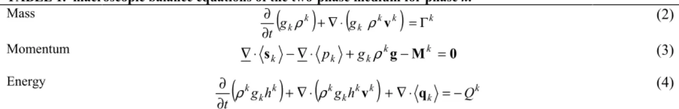
TABLE 1. macroscopic balance equations of the two-phase medium for phase k.
Mass
( ) (
k k)
k k k k g g t +∇⋅ =Γ ∂ ∂ v ρ ρ (2) Momentum ∇⋅ s −∇⋅ + kg−Mk =0 k k k p g ρ (3) Energy(
) (
)
k k k k k k k k kg h g h Q t +∇⋅ +∇⋅ =− ∂ ∂ q v ρ ρ (4)Constitutive Modelling
The spatial averaging method used in this paper is efficient to obtain in a simple way the macroscopic governing equations of the semi-solid alloy but does not enable to go further in the specifications of the macroscopic model. Reliable constitutive equations would require more sophisticated approaches such as homogenization [ 6], [ 7] associated with numerical simulation at the microscopic scale, but this is not in the scope of this work. The full definition of the two-phase model will simply be based on further constitutive assumptions.
Thermal Behavior
One important assumption of our approach is the local thermal equilibrium assumption. Such an assumption can be proved to be valid in this case according to the work of Auriault and Ene [ 8]. Actually, the liquid and the solid do not exhibit too different thermal properties nor strong thermal interfacial barriers, so at the macroscopic scale, their average temperature is the same:
T T
Ts= l= (5) A single temperature field T can therefore be defined, and the mixture energy balance can be obtained by summing equations (4) of each phase, and solved in terms of the average specific enthalpy H:
l l s sh gh g H = + (6)
This leads to the following global energy equation, which will not be further detailed in this paper.
0 = ⋅ ∇ + ⋅ ∇ + ∂ ∂ q vh h t ρ ρ (7) Mechanical Behavior
Both phases densities are considered as constant so that ρk equals ρk, its intrinsic average density. This is
valid as long as the temperature range of the solidification interval remains narrow enough. At the microscopic level, it is generally admitted that the liquid metal is an incompressible Newtonian fluid with a very low viscosity. We therefore can write:
) ( ε 2 , l l l l l l s pI with s v σ = − = µ & (8)
where pl denotes the hydrostatic pressure, sl the
deviatoric part of σσσσl, µl the viscosity of the liquid, and
) (vl
ε& the strain rate tensor. As done by Ganesan and Poirier [ 9] and Rappaz et al. [ 5], we adopt the following model for the macroscopic stress tensor:
( )
l l l l l l p g p and =− =2 ε v , Σ µ & (9)Experimental studies on the behavior of metallic alloys at high temperature show that the behavior of the solid phase is well described by constitutive equations of the Norton-Hoff type:
) ( ε ) ( eq m1 s s s s s s K p v s I s σ & & − = − = ε (10)
where K (Pa.sm) and m are the consistency and the strain rate sensitivity and ε&eq denotes the Von Mises equivalent strain rate. The behavior is then defined by
the relation between the equivalent stress (in the Von Mises sense) and the equivalent strain rate:
m eq s eq K ε
σ = & (11)
For solid fractions above the coherency fraction, using the analysis of Geindreau and Auriault [ 7], we get that the stress tensor Σs = ss − ps I+gsplI is a degree m homogeneous function with respect to the strain rate tensor ε&
( )
vs . This property shows that the solid phase can be modelled as a compressible power law fluid. We therefore adopt a compressible viscoplastic formalism [ 10], [ 1]. Constitutive equations are the ones described by (11), but with equivalents defined as( )
( )
( )
( ) ( )
(
)
(
( )
( )
)
2 3 1 9 1 1 2 2 2 ε tr : tr : s A B s s A s eq s s s s eq A B v v ε v ε Σ S S & & & & = + − + = Σ ε (12)Those equations require two rheological functions A and B that depend on the solid volume fraction and for which several models can be found [ 10], [ 1]. The constitutive equations of the solid phase at the macroscopic scale therefore read
( )
(
ε(
)
( )
εI)
Σ &εeqs 1 1A& 91B 31A tr&m s s
K + −
= − (13)
For lower solid fractions, the solid phase will be supposed to be stress free.
Momentum Exchange
According to the works of Ni and Beckermann [ 3], Mk can be partitioned as:
p k d k k M M M = + (14)
the first part being the contribution of deviatoric stresses and the second one the contribution of the isotropic part, and it can easily be shown that
0 = + d s d l M M and Mlp+Msp =0 (15) The liquid being a Newtonian incompressible fluid with a very low viscosity, we will assume that the pressure equilibrium in the liquid phase is almost instantaneous. Subsequently, the interfacial pressures in both phases (pk) equal the intrinsic average value of liquid pressure, that is its microscopic value:
l l s l p p p p = = = (16) p k
M can therefore be expressed as follows, using (1) and the general theorems of spatial averaging:
s l l l p l p s =−M =−p ∇g =p ∇g M (17)
In what follows, pl will be denoted p and referred to as the interstitial pressure.
Depending on the solid fraction, the dissipative terms Mdk are generally interpreted either as the drag force exerted by the liquid on the isolated solid grains [ 3] or the filtration force exerted by the liquid flowing through the solid, considered as a rigid porous medium [ 7], [ 5]. In both cases, M can be modelled by a law dk of the generic type:
( )
(
s)
l l l d l d s M C g v g v M =− =− − (18)where the factor C may be defined through the usual permeability factor K as:
K µ g
C= l l (19)
Mass Exchange
As proposed by Wang and Beckerman [ 4], the mass exchange term Γs=-Γl could be calculated from the species concentrations of both phases at the liquid-sold interface. Nevertheless, as first rough approach, we will assume that the solidification path is given so that the evolution of the solid fraction (2) is such as:
( )
Tt T f g g t s s s s s s ∂ ∂ ∂ ∂ = Γ = ⋅ ∇ + ∂ ∂ ρ v (20)Final Equation Set Adopted
Table 2 sums up the adopted equations set for this two-phase formulation, obtained by introducing the constitutive models in equations (2), (3) and (4). The mixture global mass conservation balance (23) was obtained by summing both phases mass balances. Because of the form of Mds (18) and of the liquid phase constitutive equations, the liquid phase motion is described through its average velocity vl , whereas the solid phase motion is described through the intrinsic average velocity vs.
TABLE 2. Final equations set of the two-phase formulation. Mechanical Problem
Momentum, solid phase ∇⋅Σ − ∇ + g+
(
v − vs)
=0 l l s s s s g C g p g ρ (21)Momentum, liquid phase ∇⋅Σ − ∇ + g−
(
v − vs)
=0 l l l l l g C g p g l ρ (22) Mass, mixture(
)
s l s s l s s l +g = − Γ ⋅ ∇ ρ ρ ρ ρ v v (23)Solid Fraction Evolution Mass, solid phase
s s s s s g t g ρ Γ = ⋅ ∇ + ∂ ∂ ( ) v (24) Thermal Problem Enthalpy, mixture 0 = ⋅ ∇ + ⋅ ∇ + ∂ ∂ q vh h t ρ ρ (25)
NUMERICAL IMPLEMENTATION
The latter formulation was implemented in the two-dimensional code R2SOL, finite element code using linear triangles and based on the P1+/P1 mixed formulation [ 12]. Up to now, the two-phase approach has been validated for isothermal situations only, so only the implementation of the isothermal mechanical problem will be discussed here. For simplicity, no gravity terms were accounted in what follows, but the extension is straightforward.
In what follows, vs will be denoted u and vl will be denoted v. The boundary conditions of the mechanical problem are
s l l l s s s u imp l imp p g p g g Ω ∂ = − ⋅ = − ⋅ Ω ∂ = = on Σ , on , T n n T n n Σ V v V u (26)
If V is the space of “kinematically admissible” velocity fields and V0 is the space of “zero kinematically
admissible” velocity fields. The virtual power principle states that the solution of the problem
(
u,v,p)
∈V×L2( )
Ω must fulfil:(
)
∈ ×( )
Ω ∀ 2 0 * * *,v ,p V L u( )
(
)
( )
(
)
( )
(
)
0 0 : Σ 0 : Σ * * * * * * * * * s = ⋅ ∇ + ⋅ ∇ − = ⋅ − ⋅ − + ⋅ ∇ − = ⋅ − ⋅ − + ⋅ ∇ −∫
∫
∫
∫
∫
∫
∫
∫
∫
Ω Ω ∂ Ω Ω Ω Ω ∂ Ω Ω Ω p g g C g p g C g p s l l l l l s l s s v u u T v u v v ε u T u v u u ε & & (27)It is a mixed velocity-pressure formulation involving two velocity fields that requires interpolation functions
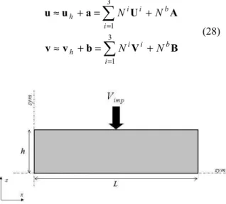
satisfying the Brezzi-Babuska conditions. Using the previous formulation developed in the one-phase case, we adopt a “(P1+)²/P1” formulation. On each finite element, the velocity fields u and v are approximated as follows: B V b v v A U a u u b i i i h b i i i h N N N N + = + ≈ + = + ≈
∑
∑
= = 3 1 3 1 (28)FIGURE 1. Two-phase simple compression test geometry.
A and B are the additional bubble degrees of freedom located at the center of each element. The bubble interpolation function Nb is linear on each sub-triangle, and is constructed such as Nb=0 on the edges of the element and Nb=1 at the center of the triangle. The interstitial pressure p is approximated by a classical linear interpolation. Weight functions u*, v* and p* are approximated in the same way. Thanks to the particular shape of the bubble functions, the additional degrees of freedom A and B can be eliminated from the discrete system at the elements level. This is obtained by the same process as the one described in [ 12] for a one-phase problem, except that the size of the local system to solve is double, due to the two
velocity fields. The resulting non linear discretized system is then solved by the means of a Newton-Raphson iterative method.
VALIDATION TESTS
Comparison With An Exact Solution
The two-phase mechanical solver was first validated with respect to an analytical solution. The latter was calculated from homogeneous simple compression problem depicted in figure 1. Both the liquid and the solid phases behavior are assumed linear and compressible:
( )
(
s s)
s s K ε I ε Σ = αtr & +β& (29)( )
(
l s)
l l b a K ε I ε Σ = tr& + & (30) gl is assumed constant over the whole domain. Thisproduces a simple compression like kinematics for both phases with an imposed strain rateε&=Vimp/h. The normal stress on each phase is supposed to be null on the right face. The resolution leads to the following expressions for the phases velocity and pressure fields:
( )
( )
( )
( )
( )
(
) ( )
− + = − − = + − = x v µ g µ p x p x v g x x v rx a x x v x s x l s s s x s x l s x , sinh 0 0 ε ε & & (31)(
)
[
]
( )
(
)
[
]
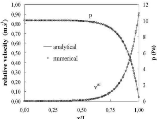
+ − = − = + + + = = ε α ε µ β β α µ µ & & b a g K K p rL r b K g K g a b a K g K g C r s l s l s s l l s s l 0 0 2 2 cosh ~ ) ( ) ( ~ ~ (32)FIGURE 2. relative velocity and interstitial pressure along the x direction, numerical vs analytical, 1D test case.
Results exposed in figure 2, correspond to a test performed at Vimp=-1m.s-1 on a sample with L=5m,
h=1m, and: gs=0.8, Ks=100 Pa.s, Kl=0.1Pa.s, α=0.189, β=0.1, a=-0.667, b=2, C=20.
As visible from figure 2, numerical results perfectly match the analytical solution both in terms of relative velocity vl /gl −vs and of interstitial pressure. Such results were obtained for several sets of rheological parameters and remain valid for any value of the interaction coefficient C.
One other important thing to check is that the formulation remains valid over the whole solidification interval, that is to say for any value of gl. Figure 3
shows the evolution of the relative velocity profile with the liquid fraction. When gl increases up to 1, the
mixture becomes more and more monophasic, which was expected. The same trend was observed for very low liquid fractions. Figure 3 thus enlighten the ability of our formulation to simulate the deformation over the whole solidification interval. It is worth noting that no special treatment was needed for the limiting cases.
Liquid Redistribution
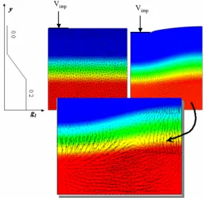
This last test aims at simulating a situation frequently encountered in continuous casting problems. It consists in imposing a deformation at the surface of a partially solidified alloy on a small part of its surface (fig. 4). It thus simulates the action of a roll. Symmetry conditions are imposed on all the boundaries except on the upper face, which is a free surface. We perform here again an isothermal calculation, but imposing an initial distribution of liquid fraction along y described in figure 4. Here, the solid phase rheology is still somewhat arbitrary, but it is now non-linear, with a strain rate sensitivity of 0.2. The interaction coefficient is modelled by a classical Carman-Kozeny law and reaches very high value in the solidified zone.
FIGURE 4. Redistribution of the liquid inside a semi-solid domain with an initial fraction distribution.
Black arrows plotted in the zoom of fig. 4 show the relative average velocity vectors vl −glvs. Results show that the applied pressure leads to a redistribution of the liquid with respect to the solid. In the zone where the solid in under pressure (left side), it undergoes densification and the liquid is rejected to the right side of the sample.
CONCLUSIONS
In this paper, the macroscopic conservation equations for a two-phase continuum have been briefly discussed and summarized. A two-dimensional finite element resolution has been proposed and validated on an analytical test. The ability of the formulation to
represent the deformation of a saturated solid skeleton, using a “sponge”-like model has been demonstrated. In the future, the model will be extended to solidification, involving mass exchange between the two phases and to the transport of chemical species, which is of great importance in casting processes.
ACKNOWLEDGMENTS
The authors would like to acknowledge the financial support of ARCELOR (represented by one of its research centers, IRSID), ASCOMETAL (from LUCCHINI group) and the french Ministère de l’Economie, des Finances et de l’Industrie, in the frame of the OSC-Continuous Casting project.
REFERENCES
1. Flemings M.C., ISIJ International, 40, 833-841 (2000). 2. Hassanizadeh M., and Gray W.G., Adv. in Water
Resources, 2, 131-144 (1979).
3. Ni J., and Beckermann C., Met. Trans. B, 22B, 349-361 (1991).
4. Wang C.Y., and Beckermann C., Metall. and Mat. Trans. A, 27A, 2754-2764 (1996).
5. Rappaz M., and Bellet M., and Deville M., Numerical modelling in materials science and engineering, New-York, Springer Verlag (2002).
6. J.-L. Auriault, E. Sanchez-Palencia, J. de Mécanique, 16, 575-603 (1977).
7. Geindreau C., Auriault J.-L., Mechanics of Materials, 31, 535-551 (1999).
8. J.-L. Auriault, H. I. Ene, Int. J. Heat and Mass Transfer, 37, 2885-2892 (1994).
9. Ganesan S. and Poirier D.R., Met. Trans. B, 21B, 173-181 (1990).
10. N’Guyen T. G., Favier D., Suery M., Int. J. of Plasticity 10, 663-693 (1998).
11. Abouaf M., and Chenot J.-L., J. Numer. Methods Eng 25, 191-212 (1988).
12. Perchat E., Fourment L., Coupez T., 3rd Conf. on Parallel and Distributed Computing for Computational Mechanics, Weimar, Germany, B.H.V. Topping Ed., Civil-Comp press, Edinburgh, pp 67-72 (1999)