A Simple Model of Foreign Brand Penetration with Multi-Product Firms: Non-Monotone Responses to Trade Liberalization

Texte intégral

(1)2011s-40. A Simple Model of Foreign Brand Penetration with Multi-Product Firms: Non-Monotone Responses to Trade Liberalization Toru Kikuchi, Ngo Van Long. Série Scientifique Scientific Series. Montréal Avril 2011. © 2011 Ngo Van Long, Toru Kikuchi. Tous droits réservés. All rights reserved. Reproduction partielle permise avec citation du document source, incluant la notice ©. Short sections may be quoted without explicit permission, if full credit, including © notice, is given to the source..

(2) CIRANO Le CIRANO est un organisme sans but lucratif constitué en vertu de la Loi des compagnies du Québec. Le financement de son infrastructure et de ses activités de recherche provient des cotisations de ses organisations-membres, d’une subvention d’infrastructure du Ministère du Développement économique et régional et de la Recherche, de même que des subventions et mandats obtenus par ses équipes de recherche. CIRANO is a private non-profit organization incorporated under the Québec Companies Act. Its infrastructure and research activities are funded through fees paid by member organizations, an infrastructure grant from the Ministère du Développement économique et régional et de la Recherche, and grants and research mandates obtained by its research teams. Les partenaires du CIRANO Partenaire majeur Ministère du Développement économique, de l’Innovation et de l’Exportation Partenaires corporatifs Banque de développement du Canada Banque du Canada Banque Laurentienne du Canada Banque Nationale du Canada Banque Royale du Canada Banque Scotia Bell Canada BMO Groupe financier Caisse de dépôt et placement du Québec Fédération des caisses Desjardins du Québec Financière Sun Life, Québec Gaz Métro Hydro-Québec Industrie Canada Investissements PSP Ministère des Finances du Québec Power Corporation du Canada Raymond Chabot Grant Thornton Rio Tinto State Street Global Advisors Transat A.T. Ville de Montréal Partenaires universitaires École Polytechnique de Montréal HEC Montréal McGill University Université Concordia Université de Montréal Université de Sherbrooke Université du Québec Université du Québec à Montréal Université Laval Le CIRANO collabore avec de nombreux centres et chaires de recherche universitaires dont on peut consulter la liste sur son site web. Les cahiers de la série scientifique (CS) visent à rendre accessibles des résultats de recherche effectuée au CIRANO afin de susciter échanges et commentaires. Ces cahiers sont écrits dans le style des publications scientifiques. Les idées et les opinions émises sont sous l’unique responsabilité des auteurs et ne représentent pas nécessairement les positions du CIRANO ou de ses partenaires. This paper presents research carried out at CIRANO and aims at encouraging discussion and comment. The observations and viewpoints expressed are the sole responsibility of the authors. They do not necessarily represent positions of CIRANO or its partners.. ISSN 1198-8177. Partenaire financier.

(3) A Simple Model of Foreign Brand Penetration with MultiProduct Firms: Non-Monotone Responses to Trade Liberalization * Toru Kikuchi †, Ngo Van Long ‡. Résumé / Abstract Nous étudions l’effet de la libéralisation du commerce international sur la prolifération des marques étrangères sur le marché du pays domestique. Les entrepreneurs du pays domestique font leur choix entre la production des produits locaux et la distribution des produits étrangers. Suite à la baisse des coûts d’importation, les importateurs élargissent l’éventail des variétés de produits importés. La croissance de la proportion des entrepreneurs qui se contentent d’importer entraine la croissance des marques étrangères sur le marché local, ce qui finalement réduit la taille de firmes importatrices. Mots clés : Marques étrangères, firmes aux produits multiples, entrepreneurs,. libéralisation du commerce international. The purpose of this study is to illustrate, using a simple model of monopolistic competition with multi-product firms, how trade liberalization affects the degree of foreign brand penetration. We model this in terms of the profit incentives for domestic entrepreneurs to choose to offer domestic brands or foreign (imported) brands, and to determine the range of varieties within each brand. As trade costs decrease, in the medium run the provider of each foreign brand will widen its range of varieties, while the provider of each domestic brand will narrow down its range of varieties. However, in the long run, more domestic entrepreneurs choose to become foreign brand providers and the range of each foreign brand becomes narrower, relative to the initial equilibrium. Keywords: Foreign brand penetration, multiproduct firms, entrepreneurs, trade liberalization, inverted J-curve effect.. *. We would like to thank seminar participants at McGill university for helpful comments. Graduate School of Economics, Kobe University, Kobe 657-8501, Japan. kikuchi@econ.kobe-u.ac.jp. ‡ CIRANO and CIREQ, Department of Economics, McGill University, 855 Sherbrooke St West, Montreal, H3A 2T7, Canada. Email: ngo.long@mcgill.ca. †.

(4) 1. Introduction. Trade liberalization through economic integration and decreasing transport and communication costs has resulted in increasing penetration of foreign brands, a phenomenon that has raised concerns among domestic producers.1 In fact, in the wake of trade liberalization, there has been not only a proliferation of foreign brands, but also a widening of varieties within each imported brand. This paper addresses both of these phenomena, using a simple model of import penetration with competition among multi-product firms to analyse short-run, medium-run, and long-run effects of decreased trade costs on product diversity (both in brand names and in varieties), relative prices, and relative profits. While trade theory has until recently used the simplifying assumption that each firm produces a single product, in practice a great deal of business transactions across national borders are conducted by multi-product firms. As Allanson and Montagna (2005) pointed out, firms can seek to create and sustain segmented market structures by pursuing differentiation strategies based on advertising, brand image, product design, styling, distribution channels, credit facilities, service arrangements and other dimensions of the total offering to customers. With a pervasive globalization mood, these tendencies are often observed for imported brands: since some specific products (e.g., French brands of perfume and wine, Italian brands of apparel) are differentiated from similar brands from other countries, firms producing (or importing) those products have stronger incentives to create and sustain segmented market structures. There are several approaches to the modelling of competition among multi-product firms. While early contributions such as Ottaviano and Thisse (1999), Ju (2003), and Allanson and Montagna (2005) modelled symmetric multi-product firms, more recent research has explored models in which heterogeneous firms produce multiple products. For example, Bernard, Redding 1. Another important aspect of foreign penetration is foreign direct investment. Ono (1990) develops an oligopoly model to deal with this point.. 3.

(5) and Schott (2010) assume that firm- and variety-specific costs are random and independent of each other, while Nocke and Yeaple (2006) assume that products are symmetric within firms, but firms differ in terms of organizational capability, which determines the rate at which the common marginal cost for each product rises with the number of products. Eckel and Neary (2010) consider a trade model of flexible manufacturing where each firm faces rising marginal costs as it offers products further away from its “core competence.” Still, the literature ignores an important aspect of real life: foreign producers and domestic sellers of foreign brands are often different entities. For example, cars are most often sold in local markets by dealers who are nationals of the importing country. As another prime example, in the Japanese apparel industry, companies such as C. Itoh and Mitsui have concentrated on licensing high-quality European and US brands. In particular, there was a large increase in the number of imported brands during the 1980s and 1990s. Commenting on this trend, Porter, Takeuchi and Sakakibara (2000) state:2 The more agreements the Japanese rivals signed, frequently with licensors based in the same countries, especially Italy, the more similar they became. As a flood of imported brands hit the Japanese market, their appeal waned. In addition, the unprecedented boom in licensed imports coincided with the peak of the bubble economy. The result: the race to sign licensing agreements ultimately destroyed industry profitability. Related to these phenomena, in a recent influential survey, Rauch (2001) argues that the difficulty of doing business across borders implies the vital role of importers (i.e., intermediaries such as Japan’s sogo shosha), particularly for trade in differentiated products. These examples seem to suggest that the focus on the “multi-product” nature of international trade should be accompanied by a focus on the behavior of domestic importing firms. In response to changes in trade costs, 2. Porter, Takeuchi and Sakakibara (2000, p. 88).. 4.

(6) entrepreneurs have incentives to switch from providing domestic brands to providing foreign brands, and to widen the range of varieties within each imported brand. The present study is designed to capture this aspect of global commerce. The main purpose of this study is to illustrate, using a simple trade model with multi-product firms operating under monopolistic competition, how trade liberalization (i.e., a decline in trade costs) can affect domestic entrepreneurs’ decision on specializing in a domestic brand or a foreign brand, as well as decision on the range of varieties within each brand. These decisions determine the degree of foreign brand penetration. Generalizing key elements of the models of Matsuyama (1995) and Allanson and Montagna (2005), we assume that there are three levels of substitutability among differentiated goods: at the level of varieties within each brand, at the brand level within each group, and finally at the group level. There are two groups of brands in the domestic market: domestic brands and foreign brands.3 Each brand is managed in this market by a domestic entrepreneur. Following Allanson and Montagna (2005), we assume that there are many differentiated varieties within a brand. Both Matsuyama (1995) and Allanson and Montagna (2005) assumed a closed economy. In contrast, in this study we focus on the case of trade and examine the effect of trade liberalization on entrepreneurs’ decision concerning (1) what kind of brands (i.e., domestic or foreign) they provide, and (2) the range of varieties for the chosen brand. The key aspect of the present study is that these two decisions are made in different time frames: while the choice of brand (i.e., movement of entrepreneurs between domestic and foreign groups) is made in the long run, the range of varieties within a chosen brand can be changed even in the medium run. On the basis of the model outlined above, this study demonstrates that, as trade costs decrease, each foreign brand provider has stronger incentives 3. Matsuyama (1995) considers only single-product firms in each of two industries, and focus on the distinction between the intra-industry elasticity of substitution and the interindustry elasticity of substitution. Allanson and Montagna (2005) consider an industry consisting of multi-product firms. These authors do not deal with international trade.. 5.

(7) to widen its range of varieties in the medium run. However, in the long run, more entrepreneurs choose to switch to become foreign brand providers; consequently, as competition among foreign brands themselves becomes tougher, each foreign brand provider begins to cut back its range of varieties. We call this phenomenon the inverted J-curve for the range of varieties within each imported brand. Nevertheless, the response of relative price is monotone: a permanent fall in trade costs by x per cent will lead in the medium run to a fall in the relative price of imported goods by γx per cent, where γ > 1, and the long run fall in relative price is by qγx per cent, where q > 1. The main results of the present study, which characterise the pattern of foreign brand penetration and the gradual shift of domestic entrepreneurs to foreign brands, have not appeared in the existing literature. Our paper is closely related to the literature on the role of entrepreneurship in trading activities. In a seminal contribution, Bond (1987) developed a two-sector model in which firms in one sector are heterogeneous due to differences in the level of ability among entrepreneurs. In a similar vein, Schmitt and Yu (2001) and Yu (2002) developed models with heterogeneous fixed export costs, which can be interpreted as differences in entrepreneurship. A potentially related literature deals with the interaction between trade liberalization and the retail market structure (Raff and Schmitt 2005, 2006, 2009). While Raff and Schmitt (2005, 2006) examine the effects of trade liberalization on markets where manufacturers have power over retailers, their third paper studies the impact of trade liberalization using an oligopoly model where retailers have market power over manufacturers. While we abstract from the market structure of retailers, our monopolistic competition model with multi-product firms are complementary to this literature in that we shed new light on the level and the composition of imported/domestic brands. The structure of this paper is as follows. In the next section we present a basic trade model of monopolistic competition with multi-product firms. The market equilibrium is presented in Section 3. In Section 4, the impact of trade liberalization is considered. Some concluding remarks are offered in. 6.

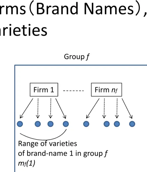
(8) Section 5.. The Model. 2. Suppose there are two countries, Home and Foreign. We assume that Foreign is large and Home is small, so that actions in Home have no impact on Foreign. This discussion will therefore concentrate on what happens in the Home (domestic) market. In Home, there are M identical individuals, each owning one unit of labor and N/M units of entrepreneurship. This implies that there are N entrepreneurs in Home.4 The representative individual consumes a numeraire good (good Z) and a collection of differentiated products. Good Z is competitively produced under constant-returns-to-scale technology: one unit of labor produces one unit of good Z (no entrepreneurship is required in this sector). Thus the wage rate is unity. On the other hand, the differentiated products, whether produced in Home or imported from Foreign for distribution in Home, require entrepreneurs who are residents of Home. Each firm needs exactly one entrepreneur. Then, at any point of time, there are exactly N firms in the differentiated-good sector in Home. Of these, nh firms produce, market, and distribute Home brand-name products, while nf firms import Foreign brand-name products from abroad and take care of their marketing and distribution in Home. Note that nf = N − nh . Entrepreneurs in the interval [0, nh ] ≡ Ih are called “domestic producers” and entrepreneurs in the interval (N − nf , N ] ≡ If are called “importers/licensees.” We assume that Foreign produces a total of NF brand-name products, where NF > N ≥ nf . In our model, NF is exogenous, while nf and nh are endogenous. Following Allanson and Montagna (2005), we suppose that each firm specializes in one brand name, and sells a continuum of varieties under that brand name (Figure 1). An entrepreneur j ∈ Ih offers mh (j) varieties un4. In what follows, the terms “an entrepreneur” and “one unit of entrepreneurship” are used interchangeably.. 7.

(9) der a Home brand name j, and produces xh (jk) units of variety k under that brand name, charging a price ph (jk) per unit. In xh (jk) or ph (jk), the index k is a real number in the continuum [0, mh (j)]. Similarly, an importer/licensee j 0 ∈ If offers mf (j 0 ) varieties under a Foreign brand name j 0 , and produces xf (j 0 k) units of variety k under that brand name j 0 , charging a price pf (j 0 k) per unit. (We will delete the prime in j 0 in what follows, to simplify notation.) Consider a representative individual resident in Home. Given any expenditure level eh (j) allocated to the goods offered by domestic producer j ∈ [0, nh ], she would allocate it among various varieties so as to maximize the following (level 1) sub-utility function, "Z. mh (j). ch (j) ≡. σ−1 σ. [ch (jk)]. σ # σ−1. dk. , σ > 1,. (1). 0. where σ > 1 is the elasticity of substitution between any two varieties within the same brand, and ch (jk) denotes consumption of a typical variety k under brand name j. Given to the sub-budget constraint Z. mh (j). [ph (jk)ch (jk)] dk ≤ eh (j), 0. the maximization of the right-hand side of (1) yields the demand functions ·. ph (jk) ch (jk) = ph (j). ¸−σ ·. where. ¸ · ¸−σ eh (j) ph (jk) = ch (j) for all k ∈ [0, mh (j)] , ph (j) ph (j) (2). "Z ph (j) ≡. 1 # 1−σ. mh (j). 1−σ. [ph (jk)]. dk. , σ > 1.. (3). 0. Note that ph (j) is dual to sub-utility function ch (j). Similarly, if the individual is to spend an amount Eh on differentiated goods produced by domestic firms, she would allocate it among the domestic 8.

(10) brands in order to maximize the following (level 2) sub-utility function, α ·Z nh ¸ α−1 α−1 , α > 1. (4) Ch ≡ [ch (j)] α dj 0. where α > 1 is the elasticity of substitution between any two brands. Given the sub-budget constraint Z nh [ph (j)ch (j)] dj ≤ Eh , 0. the solution is. ·. ph (j) ch (j) = Ph. ¸−α ·. ¸ · ¸−α Eh ph (j) = Ch for all j ∈ [0, mh ] , Ph Ph. where Ph is the group price index of Home brand-name products, 1 ¸ 1−α ·Z nh 1−α , α > 1. [ph (j)] dj Ph ≡. (5). (6). 0. Concerning the allocation among Foreign brand-name products, a similar analysis applies, with the subscript h replaced by f . Thus, · ¸−σ · ¸ · ¸−σ pf (jk) ef (j) pf (jk) cf (jk) = cf (j) for all k ∈ [0, mf (j)] , = pf (j) pf (j) pf (j) (7) 1 "Z # 1−σ mf (j) pf (j) ≡ [pf (jk)]1−σ dk , σ > 1. 0. ·. pf (j) cf (j) = Pf. ¸−α · "Z. ef Pf. ¸. N. Pf ≡. ·. pf (j) = Pf. ¸−α Cf for all j ∈ [0, mf ] .. (8). 1 # 1−α. [pf (j)]1−α dj. , α > 1.. (9). N −nf. From equations (2) and (5), and their counterparts, equations (7) and (8), the demand (per person in Home) for each variety k offered by firm j in group i is ¸−σ · pi (jk) ci (j) ci (jk) = pi (j) 9.

(11) ·. pi (jk) = pi (j). ¸−σ ·. pi (j) Pi. ¸−α. Ei = [pi (jk)]−σ [pi (j)]σ−α (Pi )α−1 Ei , i = h, f. Pi (10) Thus, for a given Ei , the demand for each variety within a brand will depend negatively on its price and positively on both the firm-level and group-level price indices, if σ > α. Now let us turn to the allocation of the consumer’s budget between the two aggregates Ch and Cf . Unlike the standard textbook monopolistic competition model where consumers do not care whether a brand is foreign or domestic, we assume that the substitutability between any two domestic brands (or between any two Foreign brands) is closer than between a domestic brand and a foreign brand. Furthermore, we assume that Home consumers may have a bias for (or against) Foreign brand-name products. Assumptions of this type have been made by a number of authors, for example Rauch and Trindade (2009), Obstfeld and Rogoff (2005, p. 88), and Warnock (2003). The consumer’s (level 3) sub-utility is represented by ε ´ ε−1 ³ ε−1 ε−1 , ε > 0, C = ah Ch ε + af Cf ε. (11). where ah > 0, af > 0, ah + af = 1, and ² is the elasticity of substitution between the domestic-brand aggregate and the foreign-brand aggregate, Ch and Cf . Given a total amount E to be spent on Ch and Cf , the relative demand will satisfy µ ¶² µ ¶−² Ch ah Ph = . Cf af Pf This condition, together with E = Ph Ch +Pf Cf , yields the demand functions Ci =. E · ³ ´1/ε ³ ´ε−1 ¸ , i = h, j. a Pi Pi 1 + aji Pj. The relative expenditure on differentiated Home goods is µ ¶² µ ¶1−² µ ¶² Ph Ch ah Ph ah Eh ≡ = ≡ ψfε−1 . Ef Pf Cf af Pf af 10. (12). (13).

(12) where ψf denotes the relative price of Foreign brand-name products, Pf /Ph .5 Equation (13) implies that the relative expenditure on group-h brands is positively related to the preference parameter (ah /af ) and positively related to the relative price of Foreign brand-name products (ψf ≡ Pf /Ph ). The expenditure share of Foreign brand-name products is denoted by µf (ψf ) : µf (ψf ) =. Ef . Ef + Eh. (14). Then, using (13), 1 Ef + Eh = =1+ µf (ψf ) Ef. µ. ah af. ¶² ψfε−1 .. (15). Thus the share µf (ψf ) is decreasing in the relative price of Foreign brandname products, µ0f (ψf ) < 0. Finally, the consumer must allocate her income, Y , between her expenditure on the homogeneous good, z, and her expenditure E on the differentiated good aggregate, C, defined by equation (11). Let us define the price index for differentiated goods by ¡ ¢ 1 P = aεh Ph1−ε + aεf Pf1−ε 1−ε . Then E = P C and the budget constraint becomes Y = z + P C. Here Y is the sum of her labor income (which is unity) and the income from her entrepreneurship. In what follows, we assume for simplicity that the utility function is u = z + log C,. (16). where z denotes the consumption of good Z. From equation (16) we obtain u = z + log E − log P . Maximizing utility subject to the budget constraint 5. Note that the group price indices Ph and Pf reflect not only the price of individual items but also the range of varieties available to consumers.. 11.

(13) E + z = Y , we obtain E = 1 (provided that Y > 1). That is, each individual spends E = 1 on differentiated goods. Thus, Home’s aggregate expenditure on differentiated goods, M E, is equal to the number of individuals, M . Our specification (16) allows us to focus on the effect of trade liberalization on the composition of demand within the differentiated good sector, abstracting from inter-sectoral reallocation of total expenditure. On the supply side of the model, in each group, differentiated products are produced at constant marginal costs (and a fixed cost) by monopolistically competitive firms. One of our central assumptions is that each brand marketed in Home must be managed by a domestic entrepreneur located in Home. Each domestic entrepreneur has to decide on what type of brand to provide. There are two options: (1) to set up a domestic firm by hiring Home labor at the wage rate wh = 1 and provide a domestic brand (i.e., to become a “domestic producer”); or (2) to set up an intermediary and import a Foreign brand for Home consumers (i.e., to become an “importer/licensee”). In the latter case, Foreign brands are assumed to be produced in Foreign by hiring Foreign labor at Foreign wage rate wf = 1. To simplify the argument, we assume that wage rates are equalized between countries, and that domestic firms in the differentiated good sector do not export. Each entrepreneur also has to decide on the range of varieties offered within the chosen brand. Following Allanson and Montagna (2005), we assume that there are fixed costs per variety. The total cost function of a typical firm j in group i that produces mi (j) varieties of products is therefore given by ! ÃZ mi (j) φi mi (j) + βi xi (jk)dk , i = h, f, 0. where φi is the fixed cost per variety in group i, βi is the firm’s marginal cost and xi (jk) is the output of variety k ∈ [0, mi (j)]. In the case of Foreign brands, φf may be interpreted as a fixed fee per variety of a given Foreign brand which the Foreign brand owner charges the domestic importer/licensee.. 12.

(14) 3. Market Equilibrium. In what follows, we distinguish short-run, medium-run, and long-run market equilibria. In the short run, both ni and mi (j) are constant. In the medium run, while ni is constant, mi (j) is variable. And in the long run, the distribution of entrepreneurs, nh and nf , is determined by Home entrepreneurs’ switching between occupations (domestic producer versus importer/licensee). Assume that the shipment of goods to consumers incur a transportation cost represented by the “iceberg” effect: for a unit of good to reach a consumer, ti units must be shipped. We assume that tf = t > 1 and th = 1, to reflect the fact that cross-border shipping is relatively more expensive (especially when one takes into account delays due to customs inspection etc.). Thus, to deliver cf (jk) units of a group-f variety, a firm in group f must ship tf cf (jk) units of it. In contrast, to deliver ch (jk) units of group-h variety, a firm in group h must ship ch (jk) units of it. Given the demand functions in (10), since there are M consumers in Home, the profit functions of a typical firm j in each group will be ÃZ ! mh (j). πh (j) = M. th Eh (Ph )α−1 [ph (j)]σ−α [ph (jk)]−σ [ρh (jk) − βh ] dk. 0. −φh mh (j), (17) ! ÃZ mf (j) α−1 σ−α −σ πf (j) = M tf Ef (Pf ) [pf (j)] [pf (jk)] [ρf (jk) − βf ] dk 0. −φf mf (j),. (18). where ρi (jk) is the mill price of variety k of firm j (i.e., brand-name j) in group i.6 The price of imported brand for Home consumers will be pf (jk) = tf ρf (jk), j ∈ If , k ∈ [0, mf (j)] . 6. (19). Recall our assumption that domestic firms in the differentiated good sector do not export.. 13.

(15) A typical firm j in group i will optimally set the mill price for each of the varieties within its brand as a constant mark up over the marginal cost βi : µ ¶ σ , ∀k ∈ [0, mi (j)] , ∀j ∈ Ii , i = h, f, ρi (jk) = βi (20) σ−1 where σ/(σ − 1) is the mark-up factor over marginal cost. Based on this pricing rule, the firm-level price index as in (3) becomes pi (j) = [mi (j)]1/(1−σ) pi (jk). Using this and (20), the profit functions, given that firms have set their prices optimally, can be re-written as 1−α. πh (j) = M Eh (Ph )α−1 [mh (j)] 1−σ βh1−α σ −α (σ − 1)α−1 − φh mh (j), πf (j) = M t1−α Ef (Pf )α−1 [mf (j)]. 1−α 1−σ. (21). βf1−α σ −α (σ − 1)α−1 − φf mf (j).(22). Assumption A1: The elasticity of substitution between any two varieties within the same brand is greater than that between any two brands, which is in turn greater that between Ch and Cf : σ > α > ε > 1. Given Assumption A1, the profit function for firm j in group i is strictly concave in its range mi (j) of varieties within its brand name. Then profit maximization with respect to mi (j) gives an interior maximum: 1−α ∂πh (j) 1−α [mh (j)] 1−σ −1 βh1−α σ −α (σ − 1)α−1 = M Eh (Ph )α−1 ∂mh (j) 1−σ −φh = 0, (23) 1−α ∂πf (j) 1−α [mf (j)] 1−σ −1 βf1−α σ −α (σ − 1)α−1 = t1−α M Ef (Pf )α−1 ∂mf (j) 1−σ −φf = 0. (24). The second order condition is satisfied since, by Assumption A1, α < σ (i.e., there is greater substitutability between any two varieties within a brand than between any two brands). In a symmetric equilibrium, all firms within the same group will have the same product range size (i.e., mi (j) = mi , ∀j ∈ Ii , i = h, f ). This then 14.

(16) implies that the group price indices in (6) and (9) can be written as µ ¶ σ 1/(1−α) 1/(1−α) 1/(1−σ) Pi = (ni ) pi (j) = (ni ) (mi ) ti βi , i = h, f σ−1. (25). where th = 1 and tf = t. Substituting (25) into (23) and (24), these first order conditions yield the symmetric equilibrium choice of mh and mf , given nh and nf : µ ¶µ ¶ M Ei 1 α−1 ∗ mi (j) = mi = (26) , j ∈ Ii , i = h, f. φi ni σ σ−1 Thus, given ni , the equilibrium range of varieties offered by a firm within a group is proportional to the expenditure level on the group’s products. Notice that while t does not appear explicitly in equation (26), it influences mi indirectly via its effect on Ei (and also, in the long run, on ni ). This will become clearer in the next section. Let us denote by rf the ratio mf to mh (the representative importer/licensee’s range of product varieties relative to that of a domestic producer), and by sf the ratio of nf to nh (the number of Home entrepreneurs who choose to be importer/licensee relative to that of domestic brand producers). We may call rf the “relative breadth” of an imported brand, and sf the “relative size” of the group of licensees. Then, from equations (13), (25) and (26), µ ∗¶ µ ¶µ ¶ mf φh nh Ef rf ≡ = ∗ mh φf nf Eh ¶ µ ¶² µ ¶(1−ε)/(1−α) µ ∗ ¶(1−ε)/(1−σ) µ ¶1−ε µ mf af nf tβf φh nh . = φf nf ah nh m∗h βh Thus # σ−1 µ ∗ ¶ " µ ¶² µ ¶ µ ¶ε−1 σ−ε mf af φh βh (α−ε)/(1−α) rf ≡ = (sf ) . (27) m∗h ah φf tβf Let the hat denote the percentage change, i.e., x b ≡ (1/x)dx for any variable x. Then, from (27), rbf = −. (ε − 1) (σ − 1) b (α − ε) (σ − 1) t− sbf . σ−ε (α − 1) (σ − ε) 15. (28).

(17) Equation (27) implies that rf is decreasing in sf . Intuitively, the more importer/licensees there are, the weaker is the incentive for each of them to offer a wide range of varieties. Then, when t falls (i.e. b t < 0), in the medium run (i.e., sf is constant), each existing importer/licensee tends to increase its range of varieties. But in the long run, this tendency will be dampened because of the (trade-liberalization-induced) increase in sf . The precise extent of this dampening effect will be computed in the next section. In equation (28), the term −(ε − 1) (σ − 1) /(σ − ε) may be called the medium run elasticity of rf with respect to trade costs, and the term − (α − ε) (σ − 1) / [(α − 1) (σ − ε)] is the elasticity of rf with respect to sf . Substituting (26) and (25) back into the profit functions in (21) and (22), we obtain the expression for the equilibrium profit πi∗ (after optimization of each firm with respect to its mi (j)) of a representative firm in group i, given nh and nf : µ ¶ M Ei 1 (σ − α) ∗ , i = h, f. πi = (29) ni σ (σ − 1) Using (29), (13), and (25), the relative profit is πf∗ = πh∗. µ. nf nh. ¶−1 µ. µ =. af ah. Pf Ph. ¶ε µ. ¶µ. nf nh. Cf Ch. ¶. µ =. ε−α µ ¶ α−1. m∗f m∗h. nf nh. ¶−1 µ. ε−1 µ ¶ σ−1. af ah. βh tβf. ¶ε µ. Pf Ph. ¶1−ε. ¶ε−1 .. (30). ³ m∗ ´ Since the ratio m∗f in (30) is endogenous in the medium run, we can replace h it using (27) to obtain the ratio of profits in the medium run πf∗ = πh∗. µ. βh tβf. µ ¶ (σ−1)(ε−1) σ−ε. af ah. µ ¶ σ−1 σ−ε. φh φf. ε−1 ¶ σ−ε. ε−α. (sf ) α−1 .. (31). The relative profit of the group of licensees is thus negatively related to the group’s relative size, sf .7 7. See Matsuyama (1995, p. 714) on this point.. 16.

(18) In the long run, the number of firms is determined by the switching of entrepreneurs across groups.8 We suppose that such switching ensures that profits in the long run are equalized between groups, π ˜h = π ˜f ,. (32). where the “tilde” indicates the long-run equilibrium value. Using (31) and (32), the long-run relative size of group-f firms, sef is sef ≡ Thus. N −n ˜h n ˜f = = n ˜h n ˜h. "µ. βh tβf. ¶ (σ−1)(ε−1) µ σ−ε. af ah. ¶ σ−1 µ σ−ε. dsef (σ − 1)(ε − 1)(α − 1) =− sef (σ − ε) (α − ε). µ. dt t. ε−1 # α−² ¶ σ−ε. α−1. φh φf. .. (33). ¶ .. (34). Proposition 1: In the long run, the relative size of group-f firms (sef ) is positively related to its relative attractiveness (af /ah ) and negatively related to trade costs, t. This implies that if there is a strong preference in favor of domestically provided brands or/and if trade costs are high, the rate of foreign brand penetration will be low.. 4. Trade Liberalization: Effects of a Permanent Fall in Trade Costs. Suppose that the system is initially at a long run equilibrium, with trade costs t > 0. Consider now a permanent reduction in trade costs: a decrease in t. We consider (a) the short-run effect [both ni and mi (j) are held constant at the initial long run equilibrium], (b) the medium-run effect [while ni is constant, mi (j) is variable], and (c) the long-run effect [both ni and mi (j) are variable], respectively. 8. Recall that total number of domestic entrepreneurs is fixed at N .. 17.

(19) 4.1. Effects on the relative price and the relative breadth of group-f firms. To see the impact of trade liberalization, let us consider the relative price of P Foreign brand-name products, ψf ≡ Phf . From (25), Pf = ψf ≡ Ph. µ. βf βh. ¶ 1. 1. (sf ) 1−α (rf ) 1−σ t.. (35). Then. 1 1 sbf − rbf + tˆ, (36) α−1 σ−1 where the “hat” indicates a percentage change. From this equation, in the short run, if the trade costs fall by x per cent, then the relative price ψf will fall by x per cent: ψbf |SR = tˆ (37) ψbf = −. where the notation SR signifies the short run, meaning that mi and ni are kept fixed. In the medium run (MR), combining (28) with (36), the relative price ψf will fall by more than x per cent when the trade costs fall by x per cent (because each existing importer/licensee begins to offer a wider range of varieties): ¶ µ ¶ µ 1 ε − 1 ψbf |M R = − rbf |M R + tˆ = 1 + tˆ σ−1 σ−ε where we have used the fact that sf is constant in the medium run, so that (28) gives (ε − 1) (σ − 1) ˆ rbf |M R = − t. σ−ε Let us turn to the long run (LR) adjustment. In the long run, the ratio nf /nh adjusts upwards as t falls (as can be seen from equation (34)), hence · ¸ (σ − 1) (ε 1 − 1) (α − 1) 1 tˆ − rbf |LR + tˆ. (38) ψbf |LR = α−1 (σ − ε) (α − ε) σ−1 18.

(20) Here, the long-run adjustment in the relative breadth (rf ≡ mf /mh ) plays an important role. From equation (28) and (34), (ε − 1) (σ − 1) b (α − ε) (σ − 1) sbf t− σ−ε (α − 1) (σ − ε) · ¸ (ε − 1) (σ − 1) b (α − ε) (σ − 1) (σ − 1) (ε − 1) (α − 1) ˆ =− t t+ σ−ε (α − 1) (σ − ε) (σ − ε) (α − ε) rbf |LR = −. =. (ε − 1)2 (σ − 1) ˆ t. (σ − ε)2. (39). This implies that, in the long run, a fall in trade costs will reduce rf . Thus we can state the following interesting results: Proposition 2 (The inverted J-curve) In the long run, a permanent fall in trade costs result in the reduction of the relative breadth of an imported brand, rf , even though in the medium run the effect is in the opposite direction. The importance of this Proposition cannot be overemphasized. When t falls, in the medium run, each existing importer/licensee tends to increase its range of varieties. But, in the long run, this tendency will be reversed because of the increase in nf /nh . Now return to the change in the relative price. Substituting (39) into (38), we can obtain the following: · ¸ (σ − 1) (ε − 1) ˆ (ε − 1)2 ˆ ˆ b ψf |LR = t+t t− (σ − ε) (α − ε) (σ − ε)2 ½ ¾ [(σ − ε) (σ − 1) − (α − ε) (ε − 1)] (ε − 1) + 1 tˆ (40) = (σ − ε)2 (α − ε) where the term inside {...} exceeds unity because σ − ε > α − ε > 0 and σ − 1 > ε − 1. Thus in the long run, the relative price ψf falls by more than x per cent when the trade costs fall by x per cent.. 19.

(21) Let us compare the medium-run effect with the long-run effect on the relative price. 1 1 sbf − rbf |LR + tˆ α−1 σ−1· ¸ 1 1 (ε − 1) (σ − 1) b (α − ε) (σ − 1) = − sbf − − sbf + tˆ t− α−1 σ−1 σ−ε (α − 1) (σ − ε) · ¸ 1 (α − ε) (σ − 1) (ε − 1) (σ − 1) b 1 1 sbf + t + tˆ = − sbf + α−1 σ − 1 (α − 1) (σ − ε) σ−1 σ−ε · ¸ 1 (α − ε) = − 1− sbf + ψbf |M R α−1 (σ − ε). ψbf |LR = −. It follows that ψbf |LR − ψbf |M R = −. · ¸ 1 (α − ε) 1− sbf . α−1 (σ − ε). (41). Thus, a permanent fall in trade costs, i.e. tˆ < 0, which increases sf (by Proposition 1), implies that the right-hand side of equation (41) is negative. We record this result in the following Proposition. Proposition 3 (Monotone fall of the relative price)The long-run percentage fall in the relative price ψf in response to a permanent x per cent fall in trade cost is larger (in absolute value) than its medium-run percentage fall. Remark: Since the price indices Ph and Pf reflect not only the prices of individual items but also both the number of brands and the range of varieties within each brand, available to consumers, the above result indicates that the expansion in the number of foreign brands more than compensate for the inverted J-curve effect in Proposition 2.. 4.2. Effects on profits. In order to examine the impact of trade liberalization, it is also useful to check the profit level of each firm (πh and πf ). Rewriting (29), and using 20.

(22) (14) the profit levels for firms are µ ¶ 1 σ−α σ−α M Eh = [1 − µf (ψf )] M E, πh = nh σ σ − 1 nh σ(σ − 1) µ ¶ 1 σ−α σ−α πf = M Ef = µf (ψf ) M E, nf σ σ − 1 nf σ(σ − 1). (42) (43). where µ0f (ψf ) < 0. Given that both ni and mi are constant in the short run, changes in short-run profit levels in response to a change in trade costs come only via changes in the relative expenditure share. Then, using (37), (42) and (43), we obtain ¸ · · ¸µ ¶ (σ − α)µ0f (ψf ) ∂πh ∂πh ∂ψf t > 0, (44) |SR = |SR = − ME ∂t ∂ψf ∂t nh σ(σ − 1) ψf ¸ ¸µ ¶ · · (σ − α)µ0f (ψf ) ∂πf ∂πf ∂ψf t |SR = |SR = ME < 0. (45) ∂t ∂ψf ∂t nf σ(σ − 1) ψf where we have made use of the fact that E = 1, regardless of t, a feature implied by our specification of the utility function (16). Via expenditure shifting from domestic brands toward imported ones, a reduction in trade costs increases the profit levels of firms in group f , while reducing the profit levels of group-h firms. From equations (44) and (45), we can state the following result: Proposition 4: In the short run, a fall in trade costs will result in an increase in each group-f firm’s profit and a decrease in each group-h firm’s profit. The ratio of the increase in πf to the decrease in πh is proportional to the inverse of the relative size of the group of licensees, nh /nf . ¯ ¯ ¯ ∂πf ¯ ¯ ∂t ¯ n 1 ¯ ∂π ¯SR = h = . h ¯ ¯ nf sf ∂t SR. In the medium run, with nf and nh remaining fixed, the expenditureshifting to imported brands induces changes in the range of varieties within 21.

(23) brand name. Since Ef becomes larger while Eh becomes smaller, each importer/licensee widens its range of varieties (mf becomes larger) while each domestic firm narrows its range of varieties [see (27)]. Thus, trade liberalization induces asymmetric responses in the breadth of varieties.9 It is important to note, from (36), this medium-run changes also increases the relative price of Home brand-name products (making them less attractive) which reinforces the short-run impact of trade liberalization. Group-h firms’ profits are further reduced by changes in ranges of their varieties, which is a natural consequences of the inverted J-curve effect in Proposition 2. Proposition 5: In the medium run, the effect of trade liberalization on relative profit of importer/licensee firms is magnified via the widening of range of varieties of each imported brand and the narrowing of range of varieties of each domestic brand. Proof: ¸ ∂πh ∂ψf |M R ∂ψf ∂t ¸µ ¶µ ¶ · (σ − α)µ0f (ψf ) ε−1 t ME 1 + > 0, = − nh σ(σ − 1) σ−1 ψf ¸ · ∂πf ∂ψf |M R = ∂ψf ∂t ¸µ ¶µ ¶ · (σ − α)µ0f (ψf ) ε−1 t ME 1 + < 0. ¥ = nf σ(σ − 1) σ−1 ψf. ∂πh |M R = ∂t. ∂πf |M R ∂t. ·. (46). (47). In the long run, entrepreneurs move from group h to group f . These movements tend to reduce the profit of each importer/licensee firm. At the new long-run equilibrium, equation (32) will be hold again. Note that the 9. From (31), the magnitude of the medium-run change of relative profit is increasing in ε, the elasticity of substitution between the domestic brand aggregate and the foreign brand aggregate.. 22.

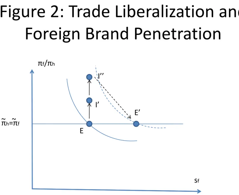
(24) profits at the new long-run equilibrium are the same as at the initial longrun equilibrium. This is because the sum of profits is depends only on E, which itself it constant because of our specification of the utility function (16). Indeed, from (42) and (43), µ ¶ 1 σ−α M E. nf πf + nh πh = σ σ−1. 4.3. Discussion. So far, we have restricted attention to a permanent fall in trade costs, from a high level to a permanent low level. However, our analysis also allows us to infer results about gradual trade liberalization. By combining Propositions 1, 4, and the above result, one can examine the short/long-run impacts of gradual trade liberalization. Suppose that trade costs decline from t to t0 first, then from t0 to t00 , and so on. As the share of imported brands increases due to trade liberalization (Proposition 1), the short-run impact of trade liberalization itself becomes smaller (Proposition 4). This implies that, as trade is gradually liberalized, the incentive for entrepreneurs to switch to provide additional imported brands becomes weaker: as a flood of imported brands hits the domestic market, their appeal wanes. Proposition 6: Suppose that trade liberalization proceeds gradually in equal steps. Then, as trade is liberalized further, the incentive for entrepreneurs to switch to the status of importer/licensee to provide additional imported brands becomes smaller. Figure 2 summarizes the discussion of this section. The horizontal axis shows the relative size of group-f firms (sf ), while the vertical axis shows the relative profit level (πf /πh ). Given that σ > α > ε and mi is constant, the relative profit level is shown as a downward-sloping curve [see, (31)]. With trade liberalization, the downward sloping curve moves upwards. The short-run equilibrium moves from point E to point I 0 . Then, in the medium 23.

(25) run, each firm responds by changing its range of varieties: this mediumrun impact is shown by a movement from I 0 to I 00 (Proposition 5), which is the reflection of the inverted J-curve effect in Proposition 2. Finally, the entrepreneurs gradually switch away from group h and the condition (32) holds again: the new long-run equilibrium is obtained at E 0 . Before closing this section, we would like to emphasize that the “foreign brand penetration” phenomenon that results from trade liberalization has two facets. On the one hand, in the medium run, each existing importer/licensee firm has incentives to increase the range of its own varieties: consumers can purchase wider range of existing Foreign brand-name varieties. On the other hand, in the long run, the number of brand names itself increases as a result of domestic entrepreneurs’ switching behavior. Then, since competition between imported brands becomes tougher, each importer/licensee begins to cut back on its own range of varieties. It is important to note that the process of foreign brand penetration is not monotone: the inverted J-curve is the outcome of the interaction between the medium-run response in product varieties within each brand, and the long-run responses of entrepreneurial switching across groups. Given that firms can change the range of varieties within each brand, the process of foreign brand penetration behaves in a complex way. In other words, differences in time frame between the range of varieties within each brand and the choice of brand itself become the source of the non-monotone outcome.. 5. Concluding Remarks. In this study, by constructing a simple monopolistic competition trade model with multi-product firms, we have highlighted the role of domestic entrepreneurs’ decision as a driving force behind a gradual foreign brand penetration. It has been shown that, as trade costs become lower, each importer/licensee chooses to broaden its range of products in the medium run. However, in the long run, since more and more domestic entrepreneurs choose to become 24.

(26) importer/licensee, the relative range of Foreign brand-name products will be narrower (Proposition 2: the inverted J-curve effect). The relative price response is monotone, despite the inverted J-curve effect. Concerning relative profits, while the widening of range of existing imported brands in the medium run magnifies the short-run impact of trade liberalization (Proposition 5), the short-run impact of trade liberalization itself becomes smaller as more entrepreneurs switch to foreign brands (Proposition 6). We would like to emphasize that the process of foreign brand penetration is non-monotone: the interaction between the medium-run response (cutting/expanding the range of varieties) and the long-run response (entrepreneurs’ switching between groups) plays an important role in determining the impact of trade liberalization. These conflicting effects of trade liberalization have not appeared in theoretical studies. This seems to suggest that incorporating multi-product firms operated by domestic entrepreneurs might be a fruitful way to deepen our understanding of the impacts of trade liberalization.. References [1] Allanson, Paul and Catia Montagna (2005) “Multiproduct Firms and Market Structure: An Explorative Application to the Product Life Cycle,” International Journal of Industrial Organization, Vol. 23, pp. 587– 597. [2] Bernard, Andrew B., Stephen J. Redding, and Peter K. Schott (2010) “Multi-Product Firms and Trade Liberalization,” (Mimeo). [3] Bond, Eric (1986) “Entrepreneurial Ability, Income Distribution, and International Trade,” Journal of International Economics, Vol. 20, pp. 343–356.. 25.

(27) [4] Eckel, Carsten and J. Peter Neary (2010) “Multi-Product Firms and Flexible Manufacturing in the Global Economy,” Review of Economic Studies, Vol. 77, pp. 188–217. [5] Ju, Jiandong (2003) “Oligopolistic Competition, Technology Innovation, and Multiproduct Firms,” Review of International Economics, Vol. 11, pp. 346–359. [6] Matsuyama, Kiminori (1995) “Complementarities and Cumulative Processes in Models of Monopolistic Competition,” Journal of Economic Literature, Vol. 33, pp. 701–729. [7] Nocke, Volker and Stephen Yeaple (2006) “Globalization and Endogenous Firm Scope,” NBER Working Paper 12322. [8] Obstfeld, Maurice and Kenneth Rogoff (2005) “Global Current Account Imbalances and Exchange Rate Adjustments,” Brookings Papers on Economic Activity 2005, No. 1, pp. 67–123. [9] Ono, Yoshiyasu (1990) “Foreign Penetration and National Welfare under Oligopoly,” Japan and the World Economy, Vol. 2, pp. 141–154. [10] Ottaviano, Gianmarco and Jacques-Francois Thisse (1999) “Monopolistic Competition, Multiproduct Firms and Optimum Product Diversity,” CEPR Discussion Paper 2151. [11] Porter, Michael E., Hirotaka Takeuchi, and Mariko Sakakibara (2000) Can Japan Compete? Cambridge, Mass.: Perseus Publishing. [12] Raff, Horst and Nicolas Schmitt (2005) “Endogenous Vertical Restraints in International Trade,” European Economic Review, Vol. 49, pp. 1877– 1889. [13] Raff, Horst and Nicolas Schmitt (2006) “Exclusive Dealing and Common Agency in International Markets,” Journal of International Economics, Vol. 68, pp. 485–503. 26.

(28) [14] Raff, Horst and Nicolas Schmitt (2009) “Buyer Power in International Markets,” Journal of International Economics, Vol. 79, pp. 437–447. [15] Rauch, James E. (2001) “Business and Social Networks in International Trade,” Journal of Economic Literature, Vol. 39, pp. 1177–1203. [16] Rauch, James E. and Vitor Trindade (2009) “Neckties in the Tropics: A Model of International Trade and Cultural Diversity,” Canadian Journal of Economics, Vol. 42, pp. 809–843. [17] Schmitt, Nicolas and Zhihao Yu (2001) “Economies of Scale and the Volume of Intra-Industry Trade,” Economics Letters, Vol. 74, pp. 127– 132. [18] Warnock, Francis E. (2003) “Exchange Rate Dynamics and the Welfare Effects of Monetary Policy in a Two-Country Model with Home Product Bias,” Journal of International Money and Finance, Vol. 22, pp. 343– 363. [19] Yu, Zhihao (2002) “Entrepreneurship and Intra-Industry Trade,” Review of World Economics, Vol. 138, pp. 277–290.. 27.

(29) Figure 1: Groups, Firms（Brand Names）, and Varieties Group f. Group h Firm 1. Firm nh. Range of varieties of brand-name 1 in group h mh(1). Firm 1. Firm nf. Range of varieties of brand-name 1 in group f mf(1).

(30) Figure 2: Trade Liberalization and Foreign Brand Penetration πf/πh I’’ I’ ~πh=π ~f. E’. E. sf.

(31)