Pépite | Détermination des sources globales d'émission d'aérosols à partir des observations satellitaires

Texte intégral

(1)Thèse de Cheng Chen, Université de Lille, 2018. THÈSE Présentée à. Université Lille 1 — Sciences et Technologies Ecole doctorale des Sciences de la Matière, du Rayonnement et de l’Environnement Par. Cheng CHEN Pour obtenir le grade de. Docteur de l’ Université de Lille 1 Spécialité:. Optique, Lasers, Physico-chimie, Atmosphère. Retrieving global sources of aerosol emissions from satellite observations Soutenance prévue le 31 janvier 2018 devant le jury composé de: Mian CHIN. Senior Scientist, NASA Goddard Space Flight Center. Rapporteuse. Gregory L. SCHUSTER. Senior Scientist, NASA Langley Research Center. Rapporteur. Lorraine A. REMER. Professor, University of Maryland, Baltimore. Exminatrice. Oliver BOUCHER. Directeur de recherche CNRS, Institut Pierre-Simon Laplace. Examinateur. Daven K. HENZE. Associate Professor, University of Colorado, Boulder. Examinateur. Didier TANRÉ. Directeur de recherche CNRS, CNRS/Université Lille1. Examinateur. Oleg DUBOVIK. Directeur de recherche CNRS, CNRS/Université Lille1. Directeur de thèse. Laboratoire d'Optique Atmosphérique U.F.R. de Physique Fondamentale Université Lille1 Sciences et Technologies 59655 Villeneuve D’ASCQ, France. © 2018 Tous droits réservés.. lilliad.univ-lille.fr.

(2) Thèse de Cheng Chen, Université de Lille, 2018. Abstract Understanding of the role that atmospheric aerosol play in the Earth-atmosphere system is limited by uncertainties in aerosol distribution, composition and sources. Thus, accurate chemical transport model simulation systems are crucial needed to analyse and predict atmospheric aerosols and their impacts on climate change and environment. Satellite observations have ability to provide an extensive spatial coverage and accurate aerosol products, however, are constrained by clear-sky condition, global coverage orbit cycle and information content. One of the most promising approaches is to reduce model uncertainty by improving the aerosol emission fields (i.e., model input) by means of inverse modeling relying on satellite observations as a constrain. In this study, we designed a method of simultaneous retrievals of desert dust, black carbon and organic carbon aerosol emission sources using aerosol data obtained from GRASP algorithm applied to POLDER/PARASOL satellite observations, and relying on the GEOS-Chem inverse modeling framework. Then, a satellite-based global aerosol emission database (2006-2011) has been developed. This aerosol emission database has been further evaluated by utilization in GEOS-Chem and GEOS-5/GOCART models. The model posterior simulation of aerosol properties employing the retrieved emissions shows a better agreement than the model prior simulation; it is true for not only fitted PARASOL products, but also for completely independent measurements from ground-based AERONET and satellites aerosol products (e.g., MODIS, MISR, OMI). The results suggest that the satellite-based aerosol emission database improves overall global aerosol modeling.. Keywords: aerosol emissions; PARASOL/GRASP; adjoint GEOS-Chem; inverse modeling; desert dust; black carbon; organic carbon.. © 2018 Tous droits réservés.. i. lilliad.univ-lille.fr.

(3) Thèse de Cheng Chen, Université de Lille, 2018. Résumé La compréhension du rôle des aérosols atmosphériques dans le fonctionnement du système terre-atmosphère est limitée par les incertitudes sur leur répartition spatiale, leur composition et leurs sources. Si leurs impacts sur le changement climatique et l’environnement peuvent être évalués grâce aux modèles de chimie-transport, ces incertitudes en limitent la précision. Les observations satellitaires ont la capacité de fournir à l’échelle globale des informations précises sur un certain nombre de paramètres « aérosols » mais elles sont limitées par les conditions nuageuses, la périodicité des orbites et par le contenu en information, c’est-à-dire le type de paramètres que l’on peut retrouver suivant la nature de ces observations. Une approche prometteuse consiste à améliorer les champs d’émission des modèles en utilisant le principe de la modélisation inverse. Dans cette étude, nous avons conçu une méthode de restitution simultanée des sources d’émission de poussières désertiques, de carbone suie et de carbone organique à partir des produits satellitaires (POLDER/PARASOL) dérivés en utilisant l’algorithme GRASP, conjointement à une modélisation inverse du modèle GEOS-Chem. Cela nous a permis de créer une base de données d’émissions globales d’aérosols sur la période 2006–2011. Des simulations réalisées avec les modèles directs GEOS-Chem et GEOS-5/GOCART utilisant cette base de données montrent bien entendu un bon accord avec des observations POLDER mais aussi une nette amélioration de la modélisation de l’aérosol à l’échelle globale lorsque l’on compare les sorties à des mesures indépendantes du réseau AERONET ou à d’autres mesures spatiales (MODIS, MISR, OMI). Mots clés: émissions d'aérosols; PARASOL/GRASP; adjoint GEOS-Chem; modélisation inverse; poussière du désert; carbone noir; carbone organique.. © 2018 Tous droits réservés.. ii. lilliad.univ-lille.fr.

(4) Thèse de Cheng Chen, Université de Lille, 2018. Acknowledgements I would like to express my sincere gratitude to many people without whom this thesis would not have been possible. Foremost, I would also particular thank my supervisor, Dr. Oleg Duvovik. He gave me a framework insight to start this scientific research and led me to appreciate the pleasure of doing research step by step. I have been very fortunate to have an excellent advisor to guide me thought my PhD. Oleg is an advisor who is really supportive not only to the scientific work but also the academic career of his students. He always encouraged and motivated me, providing me the effective point view from time to time, and correcting opportunely my mistakes. Thanks to Oleg for encouraging and supporting me to attend many conferences to present my studies and to get connected to the peers and scientists in my research fields. I sincerely appreciate the genuine support and investment Oleg has shown in my academic career. Special thanks to my thesis committee members: Dr. Mian Chin, Dr. Gregory L. Schuster, Dr. Lorraine A. Remer, Dr. Oliver Boucher, Dr. Daven K. Henze and Dr. Didier Tanré. I thank them to their careful reviews, invaluable advices and comments that helped to improve this manuscript and would be of great benefit for my future research. Daven guided me to develop the PARASOL/GRASP module on the GEOSChem adjoint modeling, and providing constructive suggestions on my manuscript and help thought my PhD. Mian encourage me to implement the retrieved aerosol emission data on other CTMs, which is the desirable goal of this thesis. I would also like to thank Tatyana Lapyonak for her continuous help of the development of the inversion model, and carefully answering my questions regarding the adjoint method used in this study. I also wish to thank her patient for revising this manuscript. I would like to acknowledge all the great help I received from people in Laboratoire d'Optique Atmosphérique. I thank Fabrice Ducos, François Thieuleux and Romain De Filippi for help in using LOA sever. I also thank Philippe Goloub, Yevgeny Derimian, Jankowiak Isabelle, Anne Priem, Marie-Lyse Liévin, Lucia Deaconu, Laura Rivellini, Ioana Popovici and Forin Unga for providing the helps not only in scientific research but also the logistics in France.. © 2018 Tous droits réservés.. iii. lilliad.univ-lille.fr.

(5) Thèse de Cheng Chen, Université de Lille, 2018. I’m highly thankful all my friends in GRASP group, including Pavel Litvinov, Benjamin Torres, David Fuertes, Anton Lopatin, Xin Huang, Qiaoyun Hu and Lei Li. I’m really lucky and enjoyable for working with you. Without supports from them, much of this work would not have been completed. Finally, to my father Guocheng Zhang, my mother Meilan Yan, my wonderful wife Fan Yang, and my nice mother-in-law Hong Li and father-in-law Bensong Yang. This work is dedicated to them.. © 2018 Tous droits réservés.. iv. lilliad.univ-lille.fr.

(6) Thèse de Cheng Chen, Université de Lille, 2018. Dedication. To my father Guocheng Zhang (张国成), my mother Meilan Yan (颜美兰), my wonderful wife Fan Yang (杨帆), and my nice mother-in-law Hong Li (李红) and father-in-law Bensong Yang (杨本松) for their constant support and unconditional love.. © 2018 Tous droits réservés.. v. lilliad.univ-lille.fr.

(7) Thèse de Cheng Chen, Université de Lille, 2018. Table of Contents Acknowledgements .......................................................................................... iii Dedication .......................................................................................................... v List of Figures................................................................................................... ix List of Tables .................................................................................................. xiv Chapter 1: General introduction ..................................................................... 1 1.1 Importance of atmospheric aerosols ............................................................................... 4 1.2 Challenges and opportunities ............................................................................................ 6 1.3 Research goals and thesis outline .................................................................................... 9. Chapter 2: Remote sensing and modeling of atmospheric aerosols ........... 11 2.1 Aerosol optical and microphysical properties .............................................................. 11 2.1.1 Aerosol Optical Depth (AOD) .................................................................................................................. 11 2.1.2 Single Scattering Albedo (SSA) .............................................................................................................. 12 2.1.3 Ångström exponent (AExp) ...................................................................................................................... 13 2.1.4 Aerosol Absorption Optical Depth (AAOD) ....................................................................................... 13 2.1.5 Aerosol complex refractive index ........................................................................................................... 13 2.1.5 Aerosol size distribution ............................................................................................................................. 14. 2.2 Aerosol remote sensing ........................................................................................................ 15 2.2.1 Ground-based remote sensing by AERONET .................................................................................... 15 2.2.2 Space-borne satellite remote sensing ..................................................................................................... 17. 2.3 Aerosol modeling ................................................................................................................... 23 2.3.1 General description ...................................................................................................................................... 24 2.3.2 Aerosol emission sources ........................................................................................................................... 28 2.3.4 Conversion of aerosol mass to optical properties ............................................................................... 33. Chapter 3: Inverse modeling and numerical tests ....................................... 38 3.1 General concept of inverse modeling .............................................................................. 38 3.2 The methodology of inverse modeling ........................................................................... 40 3.2.1 Inversion using adjoint method ................................................................................................................ 40 3.2.2 Implement a priori constrain on inversion ............................................................................................ 43. 3.3 Numerical Test ....................................................................................................................... 47 3.3.1 Inverse algorithm test over Africa ........................................................................................................... 47. © 2018 Tous droits réservés.. vi. lilliad.univ-lille.fr.

(8) Thèse de Cheng Chen, Université de Lille, 2018. 3.3.2 Inverse algorithm test for global observations .................................................................................... 57. Chapter 4: Enhance/Optimized desert dust and carbonaceous aerosol emissions over Africa ...................................................................................... 67 4.1 Introduction .............................................................................................................................. 67 4.2 Model and data description ................................................................................................ 68 4.2.1 Study Area ....................................................................................................................................................... 68 4.2.2 GEOS-Chem model and its adjoint ......................................................................................................... 70 4.2.3 PARASOL/GRASP aerosol products evaluation ............................................................................... 72. 4.3 Results ....................................................................................................................................... 74 4.3.1 Fitting of Aerosol Optical Depth ............................................................................................................. 74 4.3.2 Fitting of Aerosol Absorption Optical Depth ...................................................................................... 77 4.3.3 Emission sources ........................................................................................................................................... 79. 4.4 Evaluation ................................................................................................................................ 84 4.4.1 Evaluation with AERONET ...................................................................................................................... 84 4.4.2 Testing retrieved emission in the GEOS-5/GOCART model ........................................................ 88. 4.5 Conclusion ............................................................................................................................... 94. Chapter 5: Global desert dust and primary carbonaceous aerosol emission database (v1.0, 2006-2011) retrieved from satellite ..................................... 97 5.1 Introduction .............................................................................................................................. 97 5.2 Prior GEOS-Chem simulation of atmospheric aerosols ........................................... 99 5.3 Satellite-based emission database of BC, OC and DD ............................................ 105 5.3.1 Database description .................................................................................................................................. 105 5.3.2 Database evaluation ................................................................................................................................... 108. 5.4 Consistency with observations ........................................................................................ 110 5.4.1 Evaluation of posterior GEOS-Chem model simulation ............................................................... 110 5.4.2 Modeling applications ............................................................................................................................... 113. 5.5 Summary and discussion ................................................................................................... 117 Supplement .................................................................................................................................... 119. Conclusions and outlook .............................................................................. 123 6.1 Conclusion ............................................................................................................................. 123 6.2 Outlook and future work ................................................................................................... 126. Abbreviations and Acronyms ...................................................................... 128 References ...................................................................................................... 130. © 2018 Tous droits réservés.. vii. lilliad.univ-lille.fr.

(9) Thèse de Cheng Chen, Université de Lille, 2018. © 2018 Tous droits réservés.. viii. lilliad.univ-lille.fr.

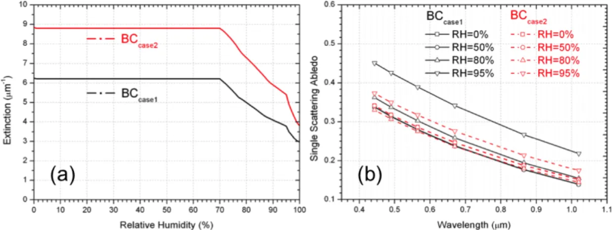
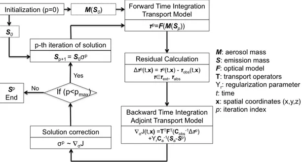
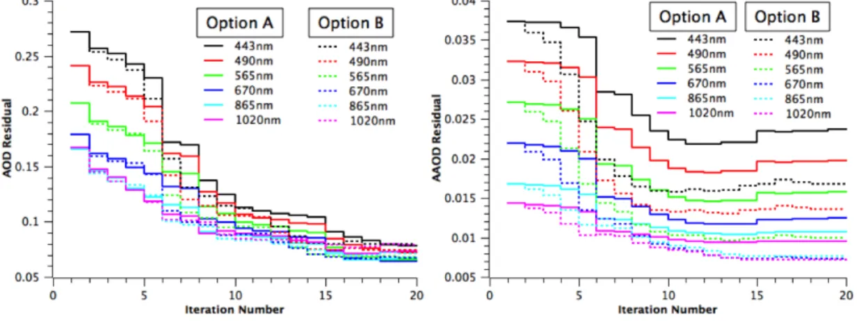
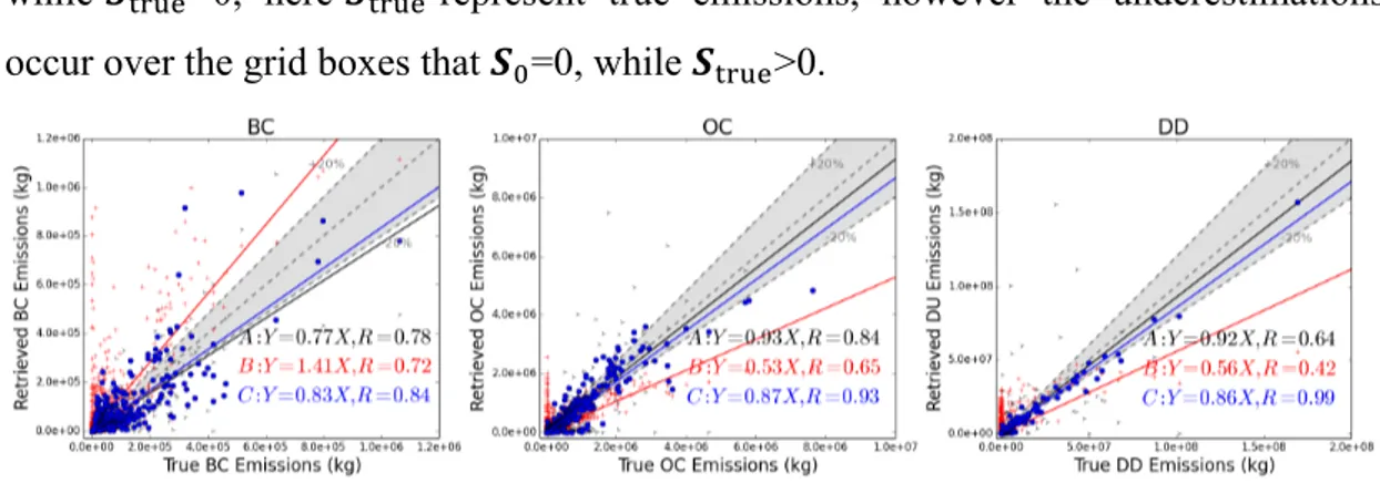
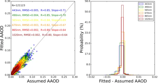
(10) Thèse de Cheng Chen, Université de Lille, 2018. List of Figures Figure 1.1: Illustration of emission, growth and removal of atmospheric aerosols, referred to Jacob, (1999). .......................................................................................................... 3 Figure 2.1: Global map of AERONET sites used in this study; the total number of daily AOD observations of a single site from 2006 to 2011 determines the size of each cross over plotted; according to the data from AERONET website: https://aeronet.gsfc.nasa.gov/ ............................................................................................... 16 Figure 2.2: The Afternoon Constellation, so-called A-Train consists of five satellites with another two failed (Glory and OCO), of spacecraft that overfly the Equator at about 1:30PM local time; adapted from https://atrain.gsfc.nasa.gov/ScienceFormationFlying.php .......................................... 19 Figure 2.3: One-box model for an atmospheric species X, refer to Jacob, (1999) ...... 25 Figure 2.4: General concept illustration of spatial and temporal discretization of the continuity equation .................................................................................................................. 27 Figure 2.5: Comparison between (a) the GOCART 2°x2.5° dust source function used in GEOS-Chem dust mobilization and (b) the GEOS-Chem annual total dust emission in 2006; Note 0.1 to 6.0µm (radius) dust particles are taken into account. ........................................................................................................................................ 29 Figure 2.6: GEOS-Chem model annual aerosol emission sources in 2006, a. sea salt, b. black carbon, c. organic carbon, d. sulfate-nitrate-ammonium; note emissions of sea salt particles for radius from 0.1 to 4.0µm are calculated. Gg (gigagram)=109 gram. ............................................................................................................. 32 Figure 2.7: (a) The relative humidity dependence of BC particle extinction at 565nm; (b) Wavelength dependence of BC particle single scattering albedo at six PARASOL wavelengths ........................................................................................................ 35 Figure 2.8: Global distribution of column integrated aerosol optical depth and aerosol absorption optical depth simulated by GEOS-Chem model at 550nm for 2006. 36 Figure 2.9: Simply classify the global aerosol type according to each component relative contribution to the total AOD and AAOD at 550nm. a. Rank 1st contributor to total AOD; b. the relative contribution of the 1st contributor to total AOD; c. rank 1st contributor to total AAOD; d. the relative contribution of the 1st contributor to total AAOD. ..................................................................................... 37 Figure 3.1: Flowchart of the general concept of inverse modeling ................................... 39 Figure 3.2: The concepts of constraining aerosol emission retrievals from satellite observations ............................................................................................................................... 44 Figure 3.3: Diagram illustrating retrieval aerosol emission sources from satellite measurements ............................................................................................................................ 46 Figure 3.4: Diagram illustrating the inversion test from synthetic measurements ....... 48 Figure 3.5: Comparison of spectral AOD and AAOD residual iteratively with two spectrum weight options ........................................................................................................ 49 Figure 3.6: Inversion test for retrieving BC, OC and DD emissions from synthetic measurements with three different initial guess schemes: (A) “prior model” emissions – “Retrieval A”; (B) Spatially uniform – “Retrieval B”; (C) Prior emission with spatially uniform background – “Retrieval C”; ................................. 51 Figure 3.7: Scatter plots between BC, OC and DD emissions retrieved from “Retrieval A, B, C” versus true values .............................................................................. 52 Figure 3.8: The differences between initial guess (from prior model) and assumed true BC, OC and DD emissions ................................................................................................... 52. © 2018 Tous droits réservés.. ix. lilliad.univ-lille.fr.

(11) Thèse de Cheng Chen, Université de Lille, 2018. Figure 3.9: Sensitivity test for retrieving DD, BC and OC emissions over 16-days with two scenarios of assumption of emission correction temporal resolution ... 54 Figure 3.10: Test of BC particle refractive index influence on the retrieval of BC emissions ..................................................................................................................................... 56 Figure 3.11: Inversion test for retrieving global BC, OC and DD emissions from synthetic measurements; (a) Assumed true dust emission; (b) Assumed true black carbon emission; (c) Assumed true organic carbon emission; (d-f) Retrieved global DD, BC and OC emissions if the retrieval ignore the contribution of sulfate and sea salt. .................................................................................... 58 Figure 3.12: Scatter plots between retrieved global DD, BC and OC emissions versus true values, the color of the points present the assumed SU+SS AOD (550nm) of this grid box ............................................................................................................................... 59 Figure 3.13: Design of a sequential approach to retrieve BC, OC and DD aerosol emission over globe; Step 1: Retrieval of BC and OC aerosol emissions from PARASOL/GRASP spectral AAOD; Step 2: Retrieval of DD aerosol emission from PARASOL/GRASP AOD (AExp<1.0) using optimized BC and OC emission from step 1 and SS and SU emission from prior model ........................... 60 Figure 3.14: Distribution of assumed 28 days mean AOD and AAOD in comparison with AOD and AAOD at 550nm simulated from initial guess of aerosol emissions, and the differences of initial guess and assumption of AOD (c) and AAOD (f) are shown. .............................................................................................................. 61 Figure 3.15: Distribution of assumed 28 days total DD, BC and OC aerosol emissions in comparison with the initial guess of DD, BC and OC emissions of our inversion ...................................................................................................................................... 62 Figure 3.16: Inversion test of using sequential approach to retrieve global DD, BC and OC aerosol emissions; a. Spatial distribution of differences between retrieval and assumed DD emission; b. Spatial distribution of differences between retrieval and assumed BC emission; c. Spatial distribution of differences between retrieval and assumed OC emission; d. Retrieved DD emission; e. Retrieved BC emission; f. Retrieved OC emission over entire 28 days; ............................................................... 63 Figure 3.17: Relative difference (%) of retrieval and assumed daily total (a) DD, (b) BC and (c) OC emissions; The mean absolute difference and the max absolute difference during 28 days are also provided in the top right of each figures. ...... 64 Figure 3.18: Illustration of fitting input PARASOL-like six wavelengths spectral AAOD of Step 1 ....................................................................................................................... 65 Figure 3.19: Illustration of fitting of input PARASOL-like six wavelengths spectral AOD of Step 2 ........................................................................................................................... 65 Figure 4.1: Distribution of PARASOL/GRASP AOD retrievals per 0.1° x 0.1° grid cell over a year (December 2007 to November 2008); the 28 AERONET sites used for validation are also shown with black cross. ................................................... 70 Figure 4.2: Validation of one-year PARASOL/GRASP spectral AOD and AAOD rescaled to 2.0° x 2.5° horizontal resolution with AERONET 28 sites measurements at 440, 675, 870 and 1020nm wavelengths over study area; The number of matched pairs (N), correlation coefficient (R), root mean square error (RMSE) and mean absolute error (MAE) are provided in the top left corner. .... 73 Figure 4.3: Comparison of the annual spatial distribution of prior (b) and posterior (c) GEOS-Chem simulated AOD at 443, 490, 565, 670 865 and 1020 nm with PARASOL/GRASP observations (a). The posterior spectral AOD are simulated using retrieved DD, BC and OC emissions. The scatter plots of grid-to-grid comparisons between PARASOL/GRASP spectral observations versus prior (d). © 2018 Tous droits réservés.. x. lilliad.univ-lille.fr.

(12) Thèse de Cheng Chen, Université de Lille, 2018. and posterior (e) GEOS-Chem simulation during one year. The correlation coefficient (R) and root mean square error (RMSE) are provide in the top left corner. .......................................................................................................................................... 76 Figure 4.4: Same as Figure 4.3 but for AAOD. ....................................................................... 78 Figure 4.5: Comparison of monthly total DD, BC and OC emissions (unit: Tg mon-1) over study area between prior model (GFED3 and Bond inventories for BC and OC, DEAD model for DD) and retrieved emissions, the annual values (unit: Tg yr-1) are provided in the top left corner. ............................................................................ 79 Figure 4.6: Spatial distribution of seasonal desert dust aerosol emission sources: (a) “prior model” DD emissions from DEAD model and (b) retrieved DD emissions. ........................................................................................................................................................ 80 Figure 4.7: Spatial distribution of seasonal BC emissions: (a) prior model BC emissions from GFED3 and Bond inventories; (b) Case 1 retrieved BC emissions; (c) Case 2 retrieved BC emissions. Note that the color scale for (b) is different from (a) and (c) for better resolving the spatial contrasts. ........................ 82 Figure 4.8: Spatial distribution of seasonal OC emissions: (a) prior model OC emissions using GFED3 and Bond inventories and (b) retrieved OC emissions. ........................................................................................................................................................ 83 Figure 4.9: Density scatter plots of one-year GEOS-Chem simulated AOD using the prior emissions (top row) or the posterior emissions (bottom row) versus AERONET measured AOD at 440, 675, 870 and 1020 nm at 28 sites. The number of matched pairs (N), correlation coefficient (R), root mean square error (RMSE) and mean absolute error (MAE) are shown on each panel. ...................... 84 Figure 4.10: Same as Figure 4.9 but for AAOD. .................................................................... 85 Figure 4.11: Time serial AOD (upper panel) and AAOD (lower pannel) from AERONET (blue crosses), PARASOL/GRASP (pink circles), Prior GEOSChem (black line) and Posterior (green line) GEOS-Chem simulations at Mongu (Zambia) site whose locations are given in Table 4.1. The statistic parameters between PARASPOL/GRASP, prior and posterior GEOS-Chem simulations with AERONET are also shown in the figure. ............................................................... 87 Figure 4.12: Time serial AOD (upper panel) and AAOD (lower pannel) from AERONET (blue crosses), PARASOL/GRASP (pink circles), Prior GEOSChem (black line) and Posterior (green line) GEOS-Chem simulations at Ilorin (Niger) site whose locations are given in Table 4.1. The statistic parameters between PARASPOL/GRASP, prior and posterior GEOS-Chem simulations with AERONET are also shown in the figure. ............................................................... 88 Figure 4.13: Comparison of the seasonal spatial distribution of prior (b) and posterior (c) GEOS-5/GOCART simulated AOD at 550 nm with MODIS observations (a). The ground-based measurements from AERONET (squares) are over plotted over figures a-c. The MODIS and GEOS-5/GOCART versus AERONET correlation coefficient (R) and root mean square error (RMSE) are provided in figures a-c. .................................................................................................................................. 90 Figure 4.14: The scatter plots of grid-to-grid comparison between MODIS and prior GEOS-5/GOCART AOD (a) and posterior GEOS-5/GOCART AOD (b) are also shown. Meanwhile, the GEOS-5/GOCART versus MODIS R, RMSE and MAE are also provided in figures (a-b). ....................................................................................... 90 Figure 4.15: Comparison of the seasonal spatial distribution of prior (b) and posterior (c) GEOS-5/GOCART simulated AAOD at 550 nm with OMI observations (a). The ground-based measurements from AERONET (squares) are over plotted over figures a-c. The OMI and GEOS-5/GOCART versus AERONET. © 2018 Tous droits réservés.. xi. lilliad.univ-lille.fr.

(13) Thèse de Cheng Chen, Université de Lille, 2018. correlation coefficient (R) and root mean square error (RMSE) are provided in figures a-c. .................................................................................................................................. 92 Figure 4.16: The scatter plots of grid-to-grid comparison between OMI and prior GEOS-5/GOCART AAOD (a) and posterior GEOS-5/GOCART AAOD (b) are also shown. Meanwhile, the GEOS-5/GOCART versus MODIS R, RMSE and MAE are also provided in figures (a-b). ........................................................................... 93 Figure 5.1: Spatial distribution of AOD (a), AAOD (b), SSA (c) and AExp (d) simulated from the prior GEOS-Chem model; the ground-based measurements from AERONET (squares) are plotted over figures a-d. The root mean square error (RMSE), correlation coefficient (R) and slope of linear regression (Slope) versus AERONET are provided in figures. ................................................................... 100 Figure 5.2: Density scatterplot (left panel) of daily PARASOL/GRASP 2°x2.5° aerosol products (AOD, AAOD, SSA and AExp) in comparison with AERONET; the correlation coefficient (R) and root mean square errors (RMSE), mean absolute error (MAE) are provided in the figures. The differences probability plots (right panel) are shown in the right column. The mean bias (MB) is provided in the top left of the figures. ............................................................ 102 Figure 5.3: Comparison of prior GEOS-Chem (GC) daily AOD with collocated AERONET (a) and PARASOL/GRASP (c) AOD at 550nm; and prior GEOSChem daily AAOD versus AERONET (b) and PARASOL/GRASP (d) AAOD at 550nm. The discriminated different aerosol types determined by the first contributor to the total AOD and AAOD are shown with color code (yellow – DD; green – OC; blue – BC; cyan – SU; purple – SS). ............................................. 103 Figure 5.4: Satellite-based global distribution aerosol emission database from 2006 to 2011, (a) black carbon, (b) organic carbon, and (c) desert dust; the annual BC, OC and DD aerosol emissions are also provided in the figure. .............................. 107 Figure 5.5: Monthly cycle of global BC (a), OC (b) and DD (c) aerosol emission from satellite-based emission database in contrast with the GEOS-Chem prior emission database; the annual trends of emissions are provided in top left of figure a-c. .................................................................................................................................. 108 Figure 5.6: Comparison of annual mean AOD, AAOD, SSA and AExp from the posterior GEOS-Chem model with AERONET between 2006 and 2011 (similar to Figure 5.1, but for posterior GEOS-Chem simulation using satellite-based aerosol emission database); ................................................................................................ 111 Figure 5.7: Comparison of posterior GEOS-Chem daily AOD and AAOD with collocated AERONET and PARASOL/GRASP at 550nm (similar to Figure 5.2, but for posterior GEOS-Chem simulation using satellite-based aerosol emission database). .................................................................................................................................. 112 Figure 5.8: Comparison of prior and posterior GEOS-5/GOCART annual mean (2006-2011) AOD at 550nm with AOD products from MODIS and MISR; (a) Prior GOCART minus MODIS AOD; (b) Prior GOCART minus MISR AOD; (c) Posterior GOCART minus MODIS AOD; (d) Posterior GOCART minus MISR AOD; ............................................................................................................................. 114 Figure 5.9: Scatter plots of prior/posterior GEOS-5/GOCART simulated AOD at 550nm in comparison with AOD from MODIS and MISR. The correlation coefficient (R), root mean square errors (RMSE), slope of linear regression (Slope), mean absolute error (MAE) and mean bias (MB) are provided in the top left of the figures. ................................................................................................................... 115 Figure 5.10: Evaluation of prior and posterior GEOS-5/GOCART AAOD at 550nm against AAOD products from OMI (OMAERUV version 1.7.4). (a)) Prior. © 2018 Tous droits réservés.. xii. lilliad.univ-lille.fr.

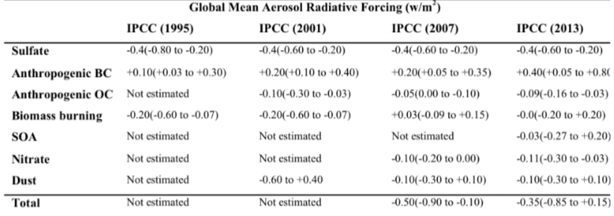
(14) Thèse de Cheng Chen, Université de Lille, 2018. GEOS-5/GOCART minus OMI AAOD; (b) Posterior GEOS-5/GOCART minus OMI AAOD; Scatter plots of prior (c) and posterior (d) GEOS-5/GOCART simulated AAOD at 550nm in comparison with AAOD from OMI. The correlation coefficient (R), root mean square errors (RMSE), slope of linear regression (Slope), mean absolute error (MAE) and mean bias (MB) are provided in the top left of the figures. ............................................................................. 116. © 2018 Tous droits réservés.. xiii. lilliad.univ-lille.fr.

(15) Thèse de Cheng Chen, Université de Lille, 2018. List of Tables Table 1.1: Estimated source strengths, lifetimes, and optical depth of major aerosol types. Statistics are based on results from 16 models examined by the Aerosol Comparisons between Observations and Models (AeroCom) projects (Kinne et al., 2006; Textor et al., 2006). ................................................................................................. 3 Table 1.2: Summary of aerosol radiative forcing (w/m2) due to aerosol-radiation interaction of seven aerosol components and comparisons between four versions of IPCC assessment reports, taken from (IPCC), (2013). .............................................. 5 Table 2.1: Summary of major satellite measurements currently available for the aerosol products ........................................................................................................................ 18 Table 2.2: Aerosol refractive index, size distribution and particle density for DD, BC, OC, SU, SS and host water employed in this study ...................................................... 34 Table 4.1: AERONET 28 sites used in this study for validation with model simulation and PARASOL/GRASP retrievals. .................................................................................... 69 Table 5.1: A summary of physical processes, emission models and inventories used in free-running GEOS-Chem simulation ............................................................................... 99 Table 5.2: A summary of the global annual DD, BC and OC aerosol emission flux from previous studies and that from this study. The unit is Tg/yr. Note that the value adopt from GEOS-Chem and GOCART model is also annual average from 2006-2011, and the dust particle size is considered from 0.1~6.0µm for GEOSChem and GOCART model. .............................................................................................. 110. © 2018 Tous droits réservés.. xiv. lilliad.univ-lille.fr.

(16) Thèse de Cheng Chen, Université de Lille, 2018. Chapter 1 General introduction. Even though the future seems far away, it is actually beginning right now. Mattie Stepanek. The atmospheric aerosol is a complex and dynamic mixture of solid and liquid particles from natural and anthropogenic sources. The amount and properties of aerosols are extremely variable in space and time. The aerosol characteristics of high interest are the size distribution, chemical composition, and shape of the particles. It is useful to classify aerosols in different categories according to these properties. There are several possible classifications.. Natural and Anthropogenic Aerosols Aerosols are produced from natural processes and anthropogenic activities. The natural sources include windborne dust, sea spray, volcanic activities and biomass burning etc., while emissions attributable to the anthropogenic activities arise primarily from fuel combustion, industrial processes, nonindustrial fugitive sources (e.g. construction work), and transportation sources (e.g. vehicles, ships). Natural aerosols are 4 to 5 times larger in amount than anthropogenic ones on a global scale, but regional variation in man-made pollution may change this ratio significantly in certain area, particularly in the industrialized Northern Hemisphere.. Primary and Secondary Aerosols Aerosols also can be divided into two classes, namely primary and secondary aerosols, according to the mechanisms of their origination. Primary aerosol particles. © 2018 Tous droits réservés.. 1. lilliad.univ-lille.fr.

(17) Thèse de Cheng Chen, Université de Lille, 2018. are emitted into the air directly. This is the case of aerosols produced by the effect of the wind friction on an oceanic or terrestrial surface and aerosols produced during an incomplete combustion. While secondary aerosol particles designate those particles that have not been emitted directly in the particulate phase but formed in the atmosphere. by. gas-particle. conversion. such. as. nucleation,. condensation,. heterogeneous and multiphase chemical reactions. Anthropogenic aerosols include primary (directly emitted) particles and secondary particles that are formed in the atmosphere from aerosol precursor gases.. Fine and Coarse Mode Aerosols The Nuclei Mode (particle diameter < 0.1µm) consists primarily of combustion particles emitted directly into the atmosphere and particles formed in the atmosphere by gas-to-particle conversion. They are usually found near highways and other sources of combustion. Because of their high number concentration, especially near their sources, these small particles coagulate rapidly. Consequently, nuclei particles have relatively short lifetimes in the atmosphere and end up in the accumulation mode. The Accumulation Mode (0.1µm < particle diameter < 2.0µm or 2.5µm) includes combustion particles, smoke particles and coagulated nuclei mode particles. Particles in this mode are small but they coagulated too slowly to reach the coarse mode. Hence, they have a relatively long lifetime in the atmosphere and they account for most the visibility effects of atmosphere. In general, the nuclei and accumulation modes together constitute “Fine Mode” aerosols. The Coarse Mode (particle diameter > 2.0µm or 2.5µm) consists of windblown dust, large sea salt particles from sea spray and mechanically generated anthropogenic particles such as those from agriculture and surface mining. Because of their large size, the coarse particles readily settle out or impact on surface, so their lifetime in the atmosphere is short. (http://aerosol.ees.ufl.edu/atmos_aerosol/section04-1.html). © 2018 Tous droits réservés.. 2. lilliad.univ-lille.fr.

(18) Thèse de Cheng Chen, Université de Lille, 2018. Figure 1.1: Illustration of emission, growth and removal of atmospheric aerosols, referred to Jacob, (1999).. Table 1.1: Estimated source strengths, lifetimes, and optical depth of major aerosol types. Statistics are based on results from 16 models examined by the Aerosol Comparisons between Observations and Models (AeroCom) projects (Kinne et al., 2006; Textor et al., 2006).. Tg (teragram)=1012 gram or 1 million metric tons The sulfate aerosol source is mainly SO2 oxidation plus a small fraction of direct emission. The organic matter source includes direct emission and hydrocarbon oxidation. Figure 1.1 illustrates the different processes involved in the aerosol emission, growth and eventual removal of different type and size of atmospheric aerosol particles. Aerosol simulation community commonly uses a discrimination of aerosol in five components: sulfate (SU), black carbon (BC), organic matter (OM), desert dust (DD) and sea salt (SS) for a better characterization of aerosol optical and microphysical properties. SS and DD contributions dominate the coarse size mode, while the fine mode is accumulated by SU, BC and OM. In addition, DD and OM. © 2018 Tous droits réservés.. 3. lilliad.univ-lille.fr.

(19) Thèse de Cheng Chen, Université de Lille, 2018. particles absorb most strongly in the UV and short wave visible channels, while BC particles are absorbing more ubiquitously (Kinne et al., 2006; Textor et al., 2006). Table 1.1 reproduced from Chin et al. (2009), presents the emissions, optical depth and life time of these five aerosol components, as represented by current aerosol transport models.. 1.1 Importance of atmospheric aerosols Atmospheric aerosols play a key role in many important environmental aspects including climate change, stratospheric ozone depletion and tropospheric air pollution. Atmospheric aerosols affect climate through three primary mechanisms (King et al., 1999). First, direct radiative forcing results when radiation is scattered or absorbed by the aerosol itself. Scattering of shortwave radiation enhances the radiation reflected back to space, therefore increasing the reflectance (albedo) of the earth and cooling the climate system. Absorption of solar and long wave radiation alters the atmospheric heating rate, which in turn may result into changes to the atmospheric circulation. Second, indirect radiative forcing results to enhance concentrations of aerosol particles and modify cloud properties, resulting in more cloud droplets, albeit smaller in size, that generally increase the albedo of clouds in the earth’s atmosphere. The indirect effect could be subdivided in two different groups: Twomey effect (Twomey, 1974, 1977) and Albreicht effect (Albrecht, 1989). In Twomey effect, aerosol influences cloud formation by providing additional nuclei for droplet of ice crystals growth (Boucher, 1999). While in Albreicht effect, aerosol effects change cloud lifetime and other cloud properties like liquid water content and cloud top height. Finally, aerosol particles could modify the atmospheric temperature profile by absorbing aerosols, and then affecting the presence of clouds. Detailed description of definition of aerosol three climate effects can be found in Haywood and Boucher, (2000). The radiative forcing (RF) is one of the ways to quantify how aerosol contributes to climate change. Aerosol radiative forcing is the net change in the energy balance of the earth system due to the presence of atmospheric aerosols. It is usually expressed in watts per square meter (𝑤/𝑚! ) averaged over a particular period of time and quantifies the energy imbalance that occurs when the imposed change take place. In the Intergovernmental Panel on Climate Change (IPCC) reports, there are RF of aerosol-radiation interaction (direct effect), RF of the aerosol-cloud interaction. © 2018 Tous droits réservés.. 4. lilliad.univ-lille.fr.

(20) Thèse de Cheng Chen, Université de Lille, 2018. (indirect and semi-direct effect) and the impact of BC particles on snow and ice surface albedo. According to the latest IPCC (2013), the total aerosol-radiation and aerosol-cloud interaction (excluding BC on snow and ice) is estimated with a 5% to 95% uncertainty between -1.9 and -0.1 𝑤/𝑚! with the best estimate value of -0.9 𝑤/𝑚! (medium confidence). Table 1.2 lists the best estimates of RF due to aerosolradiation interaction for various aerosol components taken from four versions of IPCC reports. Because absorption by ice is very weak at visible and ultraviolet wavelengths, BC in snow makes the snow darker and increases absorption. The anthropogenic BC on snow/ice is assessed to have a positive global and annual mean RF of +0.04 𝑤/ 𝑚! , with a 5% to 95% uncertainty from +0.02 to +0.09 𝑤/𝑚! (IPCC, 2013). Overall, aerosol RF can be compared in magnitude to a radiative forcing for well-mixed greenhouse gases, however the aerosol effects continue to represent one of the largest uncertainties in the detection and prediction of climate change study. Table 1.2: Summary of aerosol radiative forcing (w/m2) due to aerosol-radiation interaction of seven aerosol components and comparisons between four versions of IPCC assessment reports, taken from (IPCC), (2013).. In the short term and regional scale, aerosol particles can degrade visibility and. damage aviation and transport. The World Health Organization (WHO, 2016) has reported country estimates of air pollution exposure and its health impact, which suggests that 6.5 millions deaths (11.6% of all global deaths per year) may be associated with air pollution, and 92% of the world’s population lives in places where air quality levels do not meet the WHO ambient air quality guideline of an annual mean PM2.5 (particulate matter with a diameter of less than 2.5 microns) concentration of less than 10 𝜇𝑔/𝑚! . From this environment standpoint, aerosols still constitute an. © 2018 Tous droits réservés.. 5. lilliad.univ-lille.fr.

(21) Thèse de Cheng Chen, Université de Lille, 2018. important policy issue in air quality, and it is probably the most pressing issue in air quality regulation worldwide. Thus, knowledge of the global distribution of atmospheric aerosols is important for studying the effects of aerosols on global climate and air pollution. Thus, reliable observation and simulation systems are needed to be established to understand the role atmospheric aerosols play in earthatmosphere system (Bellouin et al., 2005).. 1.2 Challenges and opportunities At present, there are many well-established Global Circulation Models (GCMs) that simulate the global aerosol distributions by generating their own meteorology (e.g. models by Koch, 2001; Koch et al., 1999; Roeckner et al., 1996, 2003; Stevens et al., 2013; Tegen et al., 2000) and Chemical Transport Models (CTMs) that incorporate meteorological data from external sources into the model physics (e.g. models by Balkanski et al., 1993; Chin et al., 2000; Takemura et al., 2000; Ginoux et al., 2001; Bessagnet et al., 2004; Grell et al., 2005; Spracklen et al., 2005; Mann et al., 2010). However, the CTMs simulation is limited by uncertainties in knowledge of aerosol emission source characteristics, knowledge of atmospheric processes and the meteorological field data used. The large model diversity in compositional aerosol emissions, shown in Table 1.1, affects the simulation of aerosol properties. As a result, even the most recent models are mainly expected to capture only the principal global features of aerosol. For example, among different models, quantitative estimates of average regional aerosol properties often disagree by amounts exceeding the uncertainty of remote sensing of aerosol observations (Chin et al., 2002, 2014, Kinne et al., 2003, 2006; Textor et al., 2006). Therefore, there are diverse and continuing efforts to harmonize and improve aerosol modeling by refining the meteorology, atmospheric process representations, emissions and other components (e.g. aerosol aging scheme, particle mixing state etc.) (Watson et al., 2002; Dabberdt et al., 2004; Generoso et al., 2007; Ghan et al., 2007; He et al., 2016; Wang et al., 2014a, 2016). Current aerosol emission estimation is largely based on the “bottom-up” method that integrates diverse information such as population, fuel consumption in various industries and corresponding measurements of emission rates for different species (Streets et al., 2003), economic growth, and the statistics of the land use and fire burned area (van der Werf et al., 2006). While significant progress has been made. © 2018 Tous droits réservés.. 6. lilliad.univ-lille.fr.

(22) Thèse de Cheng Chen, Université de Lille, 2018. (Streets et al., 2006), the “bottom-up” approach still has a number of limitations (Xu et al., 2013): (i). The bottom-up emission inventory usually has a temporal lag of at least 2 to 3 years, because time is needed to aggregate information from different sources and format them into the emission inventories that are suitable for use in climate models.. (ii). The temporal resolution of the current bottom-up aerosol emission inventories is usually on monthly to annual scale, which is not sufficient to capture the daily or diurnal variation of aerosol distributions.. (iii). The spatial resolutions of the bottom-up emission inventories are usually limited by the availability of the external information, which often lack the spatial coverage for emission estimation in a uniformly fine resolution for regional modeling of aerosol transport.. (iv). The bottom-up emission inventories may miss important emission sources that are not well documented including emission from wild fires, volcanic eruptions, and agricultural activities.. All these limitations can be amplified in the chemical transport model simulation, because the uncertainty of aerosol emission can translate into a high uncertainty of aerosol simulation and a significant high uncertainty of aerosol climate effect evaluation. Space-borne remote sensing instruments offer an integrated atmospheric column measurement of the amount of light scattering by aerosols through modification of diffuse and direct solar radiation. Numerous satellite observations of the spatial and temporal distribution of aerosols have been conducted in the last two decades (King et al., 1999; Kaufman et al., 2002; Lenoble et al., 2013). The satellite retrievals of Aerosol Optical Depth (AOD) and Aerosol Absorption Optical Depth (AAOD) are directly related to light extinction and absorption due to the presence of aerosol particles. AOD is a basic optical property derived from many earth-observation satellite sensors, such as AVHRR (Advanced Very High Resolution Radiometer), MODIS (Moderate Resolution Imaging Spectroradiometer), MISR (Multi-angular Imaging SpectroRadiometer) and POLDER (Polarization and Directionality of the Earth’s Reflectances) (Goloub et al., 1999; Geogdzhayev et al., 2002; Kahn et al., 2009; Tanré et al., 2011; Levy et al., 2013). AAOD is another valuable product to quantify the solar absorption potential of aerosol, however only a few satellite sensors. © 2018 Tous droits réservés.. 7. lilliad.univ-lille.fr.

(23) Thèse de Cheng Chen, Université de Lille, 2018. can provide retrieval of AAOD, and only with limited accuracy, for example OMI (Ozone Monitoring Instrument) on the Aura satellite (Torres et al., 2007; Veihelmann et al., 2007) and POLDER on PARASOL (Polarization & Anisotropy of Reflectances for Atmospheric Sciences coupled with Observations from a Lidar), because only ultraviolet (UV) and shortwave visible channels and polarimetric measurements are sensitive to aerosol absorption. Despite their ability to provide a high-degree of spatial coverage, satellite measurements alone are not sufficient for answering question regarding the distributions, magnitudes, and fates of aerosols in the atmosphere. These aspects can be studied using CTMs. Combination of aerosol satellite remote sensing and aerosol model simulation can be applied for interpretation of observed spatial distributions, as observed from the satellite, and vice verse. One of the most promising approaches for reducing model uncertainty is to improve the aerosol emission fields (that is input for the models) by inverse modeling, i.e. fitting satellite observations and model estimates and by adjusting aerosol emissions. For example, Dubovik et al. (2008) developed an algorithm for inverting MODIS data and implemented the approach to retrieve distributions of aerosol emissions. The algorithm was used to implement the first formal retrieval of global emission distributions of fine mode aerosol from the MODIS fine mode AOD data. Wang et al. (2012) and Xu et al. (2013) use MODIS radiances to constrain aerosol sources over China. Huneeus et al. (2012, 2013) optimize global aerosol emission source from MODIS AOD with a simplified aerosol model (Huneeus et al., 2009). However, as discussed in works such as Dubovik et al. (2008) and Meland et al. (2013), MODIS AOD (as well as currently available aerosol satellite data) contains only limited information to evaluate aerosol types, properties, or speciated emissions. Further, inconsistencies between representations of aerosol microphysics between the CTM and the aerosol retrieval algorithm can have significant influences on inverse modeling of aerosol sources (e.g. Drury et al., 2010; Wang et al., 2010). Therefore, the retrieval of aerosol emission sources from satellite observations remains very challenging. The recently generated PARASOL/GRASP (General Retrieval of Atmosphere and Surface Properties) spectral AOD and AAOD data (Dubovik et al., 2011, 2014; data available from ICARE data distribution portal: http://www.icare.univ-lille1.fr/) present new opportunities for constraining DD, BC and OC sources because their optical properties vary dramatically in the spectrum of short wave visible to near. © 2018 Tous droits réservés.. 8. lilliad.univ-lille.fr.

(24) Thèse de Cheng Chen, Université de Lille, 2018. infrared. (VIS-NIR). viewed. by. PARASOL.. Polarimetric. remote. sensing. measurements such as those from PARASOL have been postulated to provide much greater constraints on speciated aerosol emissions and microphysical properties (Meland et al., 2013). DD aerosols are dominated by coarse mode particles, and their AOD varies slightly in the VIS-NIR spectral range; in contrast, the AOD of fine mode dominated BC and OC aerosols decrease sharply in this spectral range. In addition, DD and OC particles absorb most strongly in the UV and short wave visible channels, such as 443 nm, while BC particles are absorbing more ubiquitously (Sato et al., 2003). The GRASP retrieval overcomes the difficulty of deriving aerosol over bright surfaces in the shortwave visible wavelengths, which should help improve constraints of DD emissions over source regions, rather than having to rely on downwind observations (e.g., Wang et al., 2012).. 1.3 Research goals and thesis outline The main research goal of this PhD work is to explore the possibility of the retrieval of aerosol emission sources from recent aerosol data retrieved from the polarimetric POLDER/PARASOL produced with the GRASP algorithm. To achieve the objective, GEOS-Chem model (Bey et al., 2001) has been chosen for this study because it is the community model (http://acmg.seas.harvard.edu/geos/) with constantly maintained and improved adjoint module. The adjoint operator of GEOSChem model is realized by Henze et al. (2007). However, the current aerosol emission retrievals are limited by the information from satellite observations. The approach proposed in this work is aimed to take advantage from aerosol spectral AOD and AAOD from PARASOL/GRASP to retrieve emissions of the major aerosol types by inverting GEOS-Chem model. In order to achieve this objective, several developments were realized. First, the modeling of AOD and AAOD consistent with PARASOL/GRASP forward model was implemented in adjoint GEOS-Chem model. Second, the retrieval procedure of aerosol emissions has been set up. The procedure was designed as simultaneous fitting of spectral aerosol extinction and absorption information by adjusting the emission of the aerosol. The study was relaying on the positive heritage of inverse modeling in the previous studies (Dubovik et al., 2008; Henze et al., 2007, 2009). This PhD thesis is structured into six logical parts, each describing a milestone in the aerosol emission retrieval method development. First chapter provides an. © 2018 Tous droits réservés.. 9. lilliad.univ-lille.fr.

(25) Thèse de Cheng Chen, Université de Lille, 2018. overview of the challenges and opportunities in the field of study followed by the description of research goals and structural outline of this study. Second chapter is dedicated to the atmospheric aerosols and their properties, as well as to the aerosol remote sensing techniques both from ground base and satellites and the introduction of aerosol simulation system. Third chapter contains detailed description of the proposed retrieval methods. The retrieval method was rigorously tested by a series of sensitivity experiments, for two scenarios when the retrieval is implemented over Africa and over entire Globe. Fourth chapter is an application of designed retrieval method over Africa. It contains the detailed description of the method application over Africa, the evaluation of input PARASOL/GRASP aerosol products over Africa, and the description of retrieved one-year DD, BC and organic carbon (OC) aerosol emission. Also, the results are also validated with independent measurements. Fifth chapter discusses the efforts on applying the developed method for the generation of a six-years (2006-2011) of global dataset of aerosol emission of DD, primary BC and OC. It contains the evaluation of this PARASOL/GRASP based aerosol emission dataset and analysis of the obtained datasets compare to the existent emission datasets. Specifically, the obtained emissions were implemented in GEOS-Chem and GEOS5/GOCART (Goddard Chemistry Aerosol Radiation and Transport) chemical transport models (Chin et al., 2002, 2009, 2014; Colarco et al., 2010) and the simulated aerosol properties are validated against independent measurements from ground-based AERONET and space-borne MODIS, MISR and OMI. Sixth chapter contains the conclusions and the discussions of algorithm potential and limitations.. © 2018 Tous droits réservés.. 10. lilliad.univ-lille.fr.

(26) Thèse de Cheng Chen, Université de Lille, 2018. Chapter 2. Remote sensing and modeling of atmospheric aerosols. Research is to see what everybody else has seen, and to think what nobody else has thought.. Albert Szent-Gyorgyi. 2.1 Aerosol optical and microphysical properties Aerosol particles can be described and characterized by optical and microphysical properties. The main optical and microphysical properties of aerosols required for determining their radiation effects include the aerosol optical depth, aerosol absorption optical depth, Ångström exponent (spectral dependence of optical depth), single scattering albedo, phase matrix, complex refractive index and particle size distribution. In this section, we will describe the different aerosol properties that are used in our study.. 2.1.1 Aerosol Optical Depth (AOD) The Aerosol Optical Depth (AOD or 𝜏) (also called aerosol optical thickness, AOT, in the literature) is the measure of aerosols distributed within an integrated. © 2018 Tous droits réservés.. 11. lilliad.univ-lille.fr.

(27) Thèse de Cheng Chen, Université de Lille, 2018. atmospheric column from the Earth’s surface to the top of atmosphere, and is an extensive state parameter associated with aerosol column amount. In general, most remote sensing methods retrieve AOD. According to the Bouguer-Lambert-Beer law, the sunlight traverses atmosphere by scattering and absorption: 𝐼(𝜆) = 𝐼! (𝜆)exp [−𝑚 ∙ 𝜏 !"# 𝜆 ]. (2.1). where 𝜆 stands for wavelength, 𝐼! is the intensity of sunlight at the upper limit of the atmosphere, 𝑚 is. the. optical. air. mass. 𝑚 = 1 [𝑐𝑜𝑠𝜃! + 0.50572 ∙ 96.07995 − 𝜃!. that. !!.!"!#. can. be. approximated. as. ], here 𝜃! represents solar zenith. angle (Kasten and Young, 1989). 𝜏 !"# describes the total column optical depth and is the sum of aerosol and molecular (Rayleigh) optical depth under the cloud-free conditions: 𝜏 !"# 𝜆 = 𝜏 !"# 𝜆 + 𝜏 !"# 𝜆. (2.2). Meanwhile, optical depth of aerosols in the light path is referred to AOD and is also sum of depth of optical scattering and absorption. 𝜏 𝜆 = 𝜏! 𝜆 + 𝜏! (𝜆). (2.3). where 𝜏 represents optical depth of aerosols, 𝜏! is optical depth due to aerosol absorption (also called aerosol absorption optical depth), and 𝜏! stands for aerosol scattering optical depth.. 2.1.2 Single Scattering Albedo (SSA) Aerosol scattering albedo (SSA or 𝜔! ) is a measure of the fraction of aerosol total light extinction due to scattering, which also provides information about the absorption properties of the aerosols, and therefore it is of critical importance for quantifying the impact of aerosols on climate. The aerosol single scattering albedo is defined as the fraction of the aerosol light scattering in the total extinction: 𝜎 𝜔! = 𝜏! 𝜏 = ! (𝜎 + 𝜎 ) ! !. (2.4). where 𝜏! and 𝜏 represent aerosol scattering optical depth and aerosol optical depth respectively; 𝜎! and 𝜎! are the aerosol scattering and absorption coefficients, respectively. SSA is one of the most relevant optical properties of aerosols, since their direct radiative effect is very sensitive to it. Values of SSA range from 0.0 for totally absorbing (dark) particles to 1.0 for purely scattering particles; in nature, SSA is rarely lower than about 0.70.. © 2018 Tous droits réservés.. 12. lilliad.univ-lille.fr.

(28) Thèse de Cheng Chen, Université de Lille, 2018. 2.1.3 Ångström exponent (AExp) Ångström exponent (AExp or 𝛼) is a measure of differences of AOD at different wavelengths, which is also used to describe the dependency of the AOD, or aerosol extinction coefficient with wavelength. The AOD at two different wavelengths allows determination of Ångström exponent as follows (Ångström, (1929)): 𝛼 = −ln [𝜏 𝜆! /𝜏(𝜆! )]/ln (𝜆! 𝜆! ). (2.5). Ångström exponent relates to the sizes of aerosol particles. Namely, 𝛼 tends to be inversely dependent on particle size; larger values are generally associated with smaller aerosol particles. Basically, the values of 𝛼 less than 0.6 indicate large particles like desert dust and the values greater than 1.0 indicate small particles like sulfate, black and organic carbon particles (Eck et al., 1999; Schuster et al., 2006). Ångström exponent with combination with other parameters such as AOD and SSA are widely used for aerosol classifications in various studies (e.g. Toledano et al., 2007; Penning de Vries et al., 2015).. 2.1.4 Aerosol Absorption Optical Depth (AAOD) The aerosol absorption optical depth (AAOD or 𝜏! ) is defined as integration of the aerosol absorption coefficient of the layers 𝜎! (𝑧) over a vertical path of a light beam from the ground to the top of the atmosphere (TOA): !"#. 𝜏! =. !. 𝜎! 𝑧 𝑑𝑧. (2.6). The aerosol absorption properties are directly related to its composition, for example, most of the absorption in aerosol compound is due to presence of black carbon, absorbing mineral dust and organic/brown carbon, whereas other species (sea salt and sulfate) are predominantly non-absorbing aerosols. However, the spectral range allows discrimination between absorbing species that absorb most strongly in the UV and short visible region, such as organic/brown carbon and mineral dust, and the more ubiquitously absorbing black carbon (Sato et al., 2003).. 2.1.5 Aerosol complex refractive index The real part of complex refractive index is the ratio of light velocity in a vacuum to light velocity in this substance, which is related to light scattering. Meanwhile, the aerosol absorbing ability is determined by the imaginary part of the complex refractive index. The complex refractive index (𝑚) is expressed as:. © 2018 Tous droits réservés.. 13. lilliad.univ-lille.fr.

(29) Thèse de Cheng Chen, Université de Lille, 2018. 𝑚 = 𝑛 + 𝑖𝑘. (2.7). where 𝑛 and 𝑘 represent real and imaginary parts of refractive index, respectively. The aerosol refractive index depends on the chemical composition and the source of pollution. For example, the DD and SS aerosol, there is high spectral dependency of imaginary part. BC aerosol is the most strongly absorbers of solar radiation, furthermore the imaginary part of the complex refractive index, which is about 2 orders of magnitude higher for BC aerosol than other aerosol species. For biomass burning aerosol, the real part is ranged from 1.47 to 1.52. The refractive index of hydrophilic aerosol also depends on relative humidity (RH) decreasing with its increase.. 2.1.5 Aerosol size distribution The distribution of aerosol particle size can be represented by differential radius number density distribution, which represents the number of particles with radius between 𝑟 and 𝑟 + 𝑑𝑟 per unit volume. Hence, the total number of particles per unit volume, 𝑁! , is given by !. 𝑁! =. 𝑛 𝑟 𝑑𝑟. (2.8). !. The particle size distribution can also be approximately described using a mathematical function, such as Junge power function distribution, gamma distribution, lognormal distribution etc. According to many studies (Deshler et al., 1993; Jäger and Hofmann, 1991), the lognormal size distribution can well characterize many observed real size distributions. Variation in the number of particles 𝑛 as a function of the natural logarithm of the radius 𝑟 can be written as 𝑑𝑁 𝑁! 1 ln𝑟 − ln𝑟! 𝑛 ln𝑟 = = exp − 𝑑ln𝑟 2ln! 𝜎! 2𝜋 ln𝜎!. !. (2.9). where 𝑛 ln𝑟 is the number of particles with radius between ln𝑟 and ln𝑟 + 𝑑ln𝑟, 𝑟! is the mode radius, 𝜎! is the standard deviation of the natural logarithm of the radius (the width of the distribution) and 𝑁! is the total number of particles. Equivalent equation can be calculated for a log-normal volume density distribution, 𝑣 ln𝑟 , can be expressed as 𝑣 ln𝑟 =. © 2018 Tous droits réservés.. 𝑑𝑉 𝑉! 1 𝑙𝑛𝑟 − 𝑙𝑛𝑟! = exp − 𝑑ln𝑟 2𝑙𝑛! 𝜎! 2𝜋 ln𝜎!. 14. !. (2.10). lilliad.univ-lille.fr.

(30) Thèse de Cheng Chen, Université de Lille, 2018. where 𝑉! is the total aerosol volume per unit volume of atmosphere, 𝑟! is the mode radius for the volume size distribution and 𝜎! is the geometric standard deviation. A multi-mode distribution is simply described by a sum of several lognormal distributions. For example, the bi-modal lognormal size distribution is widely used in aerosol remote sensing and modeling. In addition, sometimes aerosol size distributions are complex superposition of more than two modes, and modern retrieval methods that allow for arbitrary shaped size distributions do retrieve distributions that would not fit a lognormal. For example, in the AERONET retrieval, volume size distribution was represented by 22 radius bins of equidistant in logarithmic scale, covering the size range from 0.05 to 15𝜇𝑚 (Dubovik and King, 2000).. 2.2 Aerosol remote sensing The global distribution of aerosols can be detected by remote sensing techniques from ground-based instruments and space-borne satellites. One of the reasons for applying remote sensing techniques to derive distribution of aerosol characteristics is to provide strong observational constrains on model depictions of global aerosol distribution (Chung et al., 2012; Sato et al., 2003).. 2.2.1 Ground-based remote sensing by AERONET The AERONET (AErosol RObotic NETwork) is a global collection of groundbased sun photometers providing reliable and accurate aerosol measurements (Holben et al., 1998), and is federation of regional and national networks deployed in the 1990s by collaboration of the National Aeronautics and Space Administration (NASA) with PHOTONS (Laboratoire d'Optique Atmosphérique-LOA, University of Lille1) in the form of automatic stations for monitoring atmospheric aerosols. The automatic sun and sky scanning radiometers are returned annually to calibration center in GSFC (Goddard Space Flight Center) and LOA for calibration against Langley calibrated reference instrument of AOD (±0.01) and a referenced integrating sphere for sky radiances (>5% absolute accuracy). For AERONET standard sun photometer (CIMEL 318), the direct sun measurements are made in several spectral channels (anywhere between 340nm and. © 2018 Tous droits réservés.. 15. lilliad.univ-lille.fr.

(31) Thèse de Cheng Chen, Université de Lille, 2018. 1640nm; 440nm, 670nm, 870nm, 940nm and 1020nm are standard). Sky measurements are performed at 440nm, 670nm, 870nm and 1020nm. The latest AERONET inversion algorithm (Dubovik et al., 2006; Dubovik and King, 2000) provides improved aerosol retrievals by fitting the entire measured field of radiances (sun radiance and the angular distribution of sky radiances) at four wavelengths (440, 670, 870 and 1020nm) to a radiative transfer model. Currently, the radiances measured by the almucantar sequence are used to make aerosol information retrieval. The radiation field is driven by the wavelength dependent aerosol complex index of refraction and the particle size distribution (in the range: 0.05 𝜇𝑚 ≤r≤15 𝜇𝑚) in the total atmospheric column. Using such a general aerosol model in the retrieval algorithm allows us to derive the aerosol properties with minimal assumptions. Only spectral and size smoothness constrains are used, preventing unrealistic oscillations in either parameter. Recent studies try to include polarimetric measurements from new CIMEL 318DP sun photometer into inversion algorithm (Fedarenka et al., 2016; Li et al., 2009b; Xu et al., 2015; Xu and Wang, 2015).. Figure 2.1: Global map of AERONET sites used in this study; the total number of daily AOD observations of a single site from 2006 to 2011 determines the size of each cross over plotted; according to the data from AERONET website: https://aeronet.gsfc.nasa.gov/. AERONET measures clear sky spectral AOD with an accuracy of ±0.02 at wavelength 440nm and ±0.01 at wavelengths ≥ 440nm (Eck et al., 1999). In addition, a number of other tendencies useful for improving retrieved aerosol properties accuracies were identified in Dubovik et al. (2000, 2002b, 2006) and Dubovik and. © 2018 Tous droits réservés.. 16. lilliad.univ-lille.fr.

(32) Thèse de Cheng Chen, Université de Lille, 2018. King, (2000). For example, the accuracy of SSA is ±0.03 when AOD>0.2. Because of consistent calibration, cloud screening and retrieval methods, uniformly acquired and processed data are available from all stations, some of which have operated for over 20 years. These data provide a high quality ground-based climatology and are suitable for long-term trend analysis over regions. For example, AERONET data have been widely used to evaluate satellite aerosol retrievals (Kahn et al., 2005; Levy et al., 2007; Remer et al., 2005). Figure 2.1 shows the global map of AERONET sites used in this study, the total number of daily AOD observations of a single site from 2006 to 2011 determines the size of each cross over plotted. Although AERONET measurements are of the highest quality to date and rapid development in last 2 decades, they are only point measurements lucking global coverage. Therefore, accurate monitoring of aerosols on a global scale still requires improving current satellite remote sensing techniques, as well as extending the surface network.. 2.2.2 Space-borne satellite remote sensing While all types of observations provide important information and help to constrain models, only satellite remote sensing has the ability to observe and quantify the aerosol distribution on a global scale. Monitoring aerosols from space has been performed for over two decades (Deuzé et al., 1999, 2001, Dubovik et al., 2011, 2014; Goloub et al., 1999; Herman et al., 2005; Higurashi et al., 1999; Hsu et al., 2004; Husar et al., 1997; Ignatov et al., 2000; Kahn et al., 2005, 2009, Levy et al., 2007, 2010, 2013, Martonchik et al., 1998, 2002, Mishchenko et al., 1999, 2007, Remer et al., 2002, 2005, Torres et al., 1998, 2007). A number of developed and launched space instruments provide global monitoring of aerosol properties. Table 2.1 summaries major passive satellite measurements available for the tropospheric aerosol characterization. The Figure 2.2 illustrates the constellation of satellites known as the “A-Train”, which are making nearly contiguous observations of many facets of the Earth system.. © 2018 Tous droits réservés.. 17. lilliad.univ-lille.fr.

(33) Thèse de Cheng Chen, Université de Lille, 2018. Table 2.1: Summary of major satellite measurements currently available for the aerosol products. Satellite aerosol retrievals have become increasingly sophisticated over the past decade. Now, satellites measure the angular dependence of radiance and polarization at multiple wavelengths from UV to the infrared (IR) at fine spatial resolution. From these observations, aerosol retrieval algorithm attempts to determine not only AOD at one wavelength, but also some information about particle size properties (size over both ocean and land). The accuracy for AOD measurements from these sensors is about 0.05 or 20% of AOD (Remer et al., 2005; Kahn et al., 2005) and somewhat better over dark water, but that for aerosol microphysical properties, which is useful for distinguishing aerosol mass types, is generally low.. © 2018 Tous droits réservés.. 18. lilliad.univ-lille.fr.