OATAO is an open access repository that collects the work of Toulouse
researchers and makes it freely available over the web where possible
Any correspondence concerning this service should be sent
to the repository administrator: [email protected]
This is an author’s version published in: http://oatao.univ-toulouse.fr/20981
To cite this version:
Atalla El-Awady Attia, El-Awady
and Duquenne, Philippe
and Le Lann,
Jean-Marc
An assessment of project complexity relyng on principal
component analysis. (2013) In: 10ème congrès international de génie
industriel, CIGI-2013, 12 June 2013 - 12 June 2013 (La Rochelle, France).
(Unpublished)
EL-AWADY ATTIA
1, PHILIPPE DUQUENNE
2, JEAN–MARC LE-LANN
3 1,2,3UNIVERSITE DE TOULOUSE/ INPT/ ENSIACET/ LGC-UMR-CNRS 5503/PSI/ GENIE INDUSTRIEL
4 allée Emile Monso – BP 44362, 31030 Toulouse cedex 4.
{elawady.attia,Philippe.Duquenne,JeanMarc.Lelann}@ensiacet.fr
A
N ASSESSMENT OF PROJECT COMPLEXITY RELYING ON
Résumé – L’évaluation de la complexité du projet est très important pour prédire le résultat de planification d'un projet et
/ ou pour le bien contrôler. L'évaluation de cette complexité semble difficile, surtout avec la présence de flexibilités du temps de travail ainsi que la polyvalente des effectifs avec productivité hétérogène qui diffère de compétence à l’autre. Dans cet article, nous présentons un ensemble de mesures différentes qui peuvent être utilisées pour quantifier les nombreuses caractéristiques d'un projet et les ressources demandés. Par conséquent, les quantificateurs les plus importantes du réseau concernant sa taille, de dépendances, de la forme, l’asymétrie et son goulot d'étranglement seront présentés. En outre, les quantificateurs relatifs aux caractéristiques temporelles, la charge des travaux, et la disponibilité des ressources seront également présentées et discutées. S’appuyant sur la version normalisée de ces différentes mesures et en utilisant un ensemble de données de 400 projets avec une description différente des charges de travaux et les disponibilités des ressources, des indices agrégés de complexité du projet seront produits. Les agrégations linéaires de ces indices ont été réalisées en utilisant l’analyse en composantes principales. Par la suite, ces indices ont été utilisés pour évaluer la performance et la robustesse d'une approche méta-heuristiques qui a utilisé des algorithmes génétiques. L’analyse des résultats a montré l’efficacité de certains des indices proposés pour expliquer les variances des résultats de l’ensemble de 400 projets. Par ailleurs, l’un de ces indices que nous avons appelé «indice de poids de projet», peut être utilisé efficacement pour prédire la présence de pénalités de retard ou de la non-capacité à réaliser le projet avec les ressources pendant la durée contractuelle spécifiée.
Abstract – The assessment of project complexity is very important in order to predict the outcome of a project scheduling
and/or controlling it. The evaluation of this complexity seems difficult especially with the presence of working time flexibilities as well the multi-skilled workforce with heterogeneous productivity level that differs from skill to another. In this paper, we present a group of different measures that can be used to quantify the numerous characteristics of a project and the required resources. Therefore, the most significant quantifiers of the network regarding to its size, dependencies, shape, asymmetry, and its bottleneck will be presented. Moreover, the quantifiers related to the temporal characteristics, work-content, and availability of resources will also be discussed and presented. Relying on the normalised version of these different measures and using a data set of 400 projects with different description of work-content and resources availabilities, the smallest number of project complexity indices will be produced. The linear aggregations of these indices were conducted using the principal component analysis. Subsequently, these indices were used in evaluating the performance and robustness of a metaheuristics approach that used genetic algorithms. The result analysis showed the effectiveness of some of the proposed indices to explain the most variance of different outcomes of the data set of 400 projects. Moreover, one of these indices that we called “project weight index”, can be used efficiently to predict the presence of lateness penalties or the un-capability to realise the project with the specified resources during the specified contractual duration.
Mots clés – Gestion du projet, Ressources humaines, évaluation de la complexité, analyse en composantes principales. Keywords – Project management, Human resources, complexity assessment, principal component analysis.
INTRODUCTION
Complex project schedules can complicate the process of planning and coordinating project activities, the need of measuring schedule complexity is essential since what cannot be measured cannot be controlled or improved (Bashir and Thomson, 1999). But, project complexity is often recognized in a general way, but not completely understood by everyone (Ireland, 2007), moreover there is a mix between measuring the project schedule complexity and the project complexity itself, (Mo et al., 2008). (Ireland, 2007) explained his idea by defining the word complex, where, “Complex” comes from the Latin word complexus, meaning entwined, twisted together, also defined as an aggregate of parts. This interpretation of the complexity is aligned with that of (Nassar and Hegab, 2008): the project overall complexity is an aggregation of a set measures, such as schedule complexity, resources, cash requirements, technical and technological issues, workforce issues…etc. Despite the difficulties associated to assess scheduling complexity, measuring them can be useful in many
directions, e.g. evaluation of scheduling algorithms
performance, comparison between different algorithms. The assessment of the project network complexity can be used also in supply chains (Modrak and Semanco, 2011), concurrent engineering (Haberle et al., 2000), industrial process (Modrak, 2006), or any application used directed graphs.
Concerning the problem of project scheduling with resources constraints, measuring its complexity can be relying on a set of different attributes related to activities and resources. Thus, after scaling of these quantifiers, the ease of performing or not a given programme of activities can be measured. These quantifiers can be grouped according to the problem dimensions which contributes in forming the project and so its complexity. Generally they can be divided into three groups: the first is related only to the project, the second is purely related to the available resources (qualitative and quantitative), and the third refluxes the complexity produced from the interaction between project and capacities of available resources “project weighting”. We classified the project parameters into three main groups: network related parameters; temporal related parameters, and work-content related parameter. For other classifications one can find the work of (Patterson, 1976), (Elwany et al., 2003) (Browning and Yassine, 2009).
But what are the characteristics of a good measure? (Latva-Koivisto, 2001) discussed some criteria of a network complexity measure which include the following: – Validity: the measure measures what it is supposed to measure. – Reliability: The measures obtained by different observations of the same process are consistent. – Computability: A computer program can calculate the value of the measure in a finite time, and preferably quickly. – Ease of implementation: the difficulty of implementation of the method that computes the
complexity measure is within reasonable limits. –
Intuitiveness: it easy to understand the definition of the measure and see how it relates to instinctive notion of complexity. – Independence of the other related measures: Ideally, the value of the complexity measure is independent of other properties that are sometimes seen are related to complexity, these include at least size and visual representation of the process. Moreover and based on the work of (Thesen, 1977), we added another characteristics such as its sensitivity and “Referential”. “Referential” means that the measure should be normalised over a given period, the lower limit represent the easiest case, and upper limit indicate the hardest case of the problem. The need of a “Referential” guides is to
differentiate between the easy and the hard instances of a given problem.
In this article, the most measures of project scheduling complexity are presented. Moreover, some measures are developed in order to characterise the problem of flexible man-task allocation. This problem mainly characterised by two flexibility dimensions: -the first is the multi-skilled workforce with heterogeneous productivities on the operator level or the skill level. That is to say, the productivity of the same actor fluctuates from skill to skill, and the performance of all operators can be fluctuated in performing the same skill. -The second dimension is the flexible working time under annual hours. As previously mentioned, the complexity is by default an aggregation of different aspects, so we developed new linear composite measures to quantify the project complexity. We propose to aggregate the different correlated attributes to the smallest number of non correlated indexes relying on the principal component analysis “PCA”. The main contribution of this work is the integration of different aspects of the same project dimension (tasks dependencies, work-content, and resources nature). Moreover to the novel applicability of the proposed aggregation tool “PCA” to the assessment of project complexity. In addition, an application of the proposed indices will be presented. Finally, we propose sensitive indices that can used to represent the project relying on all of its dimensions.
We organized our article as follows: in section 2, we present the problem. Section 3 discusses and investigates the different project network measures. Section 4 investigates the project temporal measures. Section 5 discussed the different workload measures. The proposed resources measures discussed in section 6. And section 7 presents the project load density measures. Section 8 presents the proposed aggregation method relying on PCA. An application of the proposed aggregated indices will be presented in section 9. And finally, the conclusions and directions of further research are presented in Section 10.
PROBLEM DESCRIPTIONS
We are interested to measure the complexity of a resource constrained problem that can be presented as follows: A project consists of a set I of unique and original tasks with specified temporal relations. We only consider one project at a time. The execution of each task i I requires a given set of skills taken within a group K of all the skills present in the company. The duration of the task is unknown in advance, we have only three estimated values [Dimin, Di, Dimax] respectively corresponding to [minimum, standard, maximum]. In the other side, the resources are a set A of human resources, each employee “a” (we call him actor) being able to perform one or more skill(s) “from the set K, with a time-dependent performance – we consider this actor as multi-skilled. The ability of each worker “a” to practice a given skill “k”, is expressed by an efficiency θa,k in the range [0,1]; if the actor has an efficiency θa,k = 1, he is considered to have a nominal competence in the skill “k”. So when this actor is allocated for this skill on any task, he will perform the work-content in the standard workload’s duration, whereas other actors, whose efficiencies are lower than (1.0) for this skill, will require a longer working time. Resulting in an increase of both execution time and labour cost, we assume that actors’ wages are the same. From this point of view, the actual execution duration of a work content related a skill of a given task is not
predetermined: it results from the decisions about actors’ allocations. Indeed, in this problem θa,k
[θkmin, 1], whereθkmin represents the lower limit below which the allocation is not considered as acceptable, for economic and/or quality reasons. Moreover, this efficiency is dependent on the work practicing, i.e. it will be developed due to learning by doing or degrade due to work interruption. In addition to the actors’ versatility, we consider that the company adopts a working time modulation strategy: the timetables of its employees may be changed according to the workloads to be done. But each worker has a fixed amount of working hours per year that can be irregularly spread. Each individual can have his own timetable, which can vary on daily or weekly bases. This variation should obey some pre-specified milestones, as the minimum/maximum number of working hours per day, a maximum number of working hours per week, and a maximum number of average working hours per a number of weeks, called the reference period (implicitly 12 weeks, according to the French working law), for more details see the work of (Attia et al., 2011)(Attia, Edi, et al., 2012).
PROJECT NETWORK PARAMETERS
1.1 Project network size
The number of tasks/nodes is one of the essential parameters that were previously used in almost all the publications, especially in the context of the problems that can be represented by a network, as example in RCPSP (Kolisch et al., 1995), (De Reyck and Herroelen, 1996a)(Valadares Tavares et al., 1999)(Mendes et al., 2009), assembly line balancing problem (Otto et al., 2011), supply chain, transportation problems ...etc. It was used by (Valadares Tavares et al., 2002), as one of their study indicators to present the project size, in order to compare between the available benchmark problems and/or data generators of (Patterson, 1984), (Kolisch et al., 1995), (Agrawal et al., 1996), (Valadares Tavares et al., 1999). As they noted the project networks with more than 200 activities are most common in any engineering field. Therefore we used as one of the project size quantifiers. To normalize it over the interval [0, 1], we can use the correlation: P-Size= (2/ (1+e-log(I))-1) for I ≥ 1, it
reaches the unity value when I reaches infinity, for only one activity project it has a value of zero.
1.2 Project network topology
The word topology here is the study of continuity and connectivity; it is also used to refer to the structure. Measuring this network factor has a great attention from researches since the mid-sixties, where it used to represent the level of interconnection and/or interdependence between the project activities. It can also directly reflex the complexity degree in the schedule of the project or the combinatorial complexity of the network; so it can be used as a sensation tool for the difficulty of analysis a given project network. We will adopt the use of this parameter as one of the factors which measure the project scheduling complexity. This agreement is aligned with that of (Nassar and Hegab, 2008). In literature, this measure was used as one of the predictors of the processing or computational time required by certain software, or simply to compare the performance of two algorithms in resolve a given problem. It is often known as network complexity of the project. (Nassar and Hegab, 2006) adopted the use of it as an indicator for the time required during schedule or planning of the project when they used specific software. Obviously, the more interdependence between project activities, the more
complex the schedule will be, but it is not always true according to (De Reyck and Herroelen, 1996b) (Latva-Koivisto, 2001), they proved that as the tasks independents increased the network become easier to be solved especially for the RCPSP. In addition to the use of heuristic algorithms in the study of (Alvarez-Valdes and Tamarit, 1989), they said that the complexity of the project graph has a direct influence on the quality of the solution, and when the number of arcs per activity increases the problem become easier and the solution obtained is better. But others like (Valadares Tavares et al., 2002) and (Browning and Yassine, 2009) stated the contrary, e.g (Browning and Yassine, 2009) stated that “A greater
number of relationships among the activities (higher complexity) leaves less flexibility for doing them at a different time (because more things must happened before them, and more things depend on them before occurring)”. Whatever, we
consider this measure as one of the project indicators, in addition, we agree with (Elmaghraby and Herroelen, 1980)(De Reyck and Herroelen, 1996b) (Nassar and Hegab, 2008): it is not sufficient to judge the complexity of a given project scheduling according to the network structure and neglect all of other parameters.
Many correlations have been presented to measure the nature of projects’ networks structure; here we will discuss and compare some of the previously developed measures for activity on nodes (AoN). Considering that the most methods of project management represent the project network using the (AoN) notations.
1.2.1 Coefficient of Network Complexity (CNC)
(Kaimann, 1974) presented a measure of the network
complexity either for AoN/AoA networks, it can be calculated in function of the number of arcs “NA” and the nodes “NN”: as: CNC=NA2/NN. Regardless the drawbacks of the CNC corresponding its insensitivity, and based on the consideration of “The redundant arcs should not increase a network’s complexity” (Kolisch et al., 1995) in their project generator of (AON) networks “PROGEN”, adopted the network complexity measure of (Kaimann, 1974) by considering only the non-redundant arcs. This network complexity measure (known here as C) was presented as the average number of non-redundant arcs per node (including the fictive super-source and the sink). Moreover, (Nassar and Hegab, 2006) adopted it to represent a project network complexity measure based only the number of project activities and the number of edges. This measure was developed as an add-in to commercial scheduling software “MS project”. They proposed to determine the maximum and minimum number of edges possibly in the network with a given number of activities. Then the complexity of any network can be assessed in relation to those upper and lower bounds of network edges number. Then based on the logarithmic projection they introduced the percentage of the network complexity within the interval [0, 100]. Other linear projection was proposed by (Mo et al., 2008) for the same measure of (Nassar and Hegab, 2006). As they discussed the limitation of this tool is its locality i.e. it is best used to compare and asses schedule networks for a single unique project. In addition, redundant edges should be eliminated before computing the network complexity. Fortunately, (Bashir, 2010) proposed a methodology adopted from the Interpretive Structural Modeling “ISM” that transfers the AON project network into a minimum-edge diagraph which contains no redundant relationships.
1.2.2 Number of maximum generating trees:
(Temperley, 1981) introducing a classification of graphs based on their connectedness quantified complexity; he proposed to use the number of distinct trees that a graph contains as the measure of its complexity. The number of distinct trees that a graph contains (NT) is calculated using so-called tree-generating determinant (DetII). This determinant can be calculated for any graph containing no cycles and not more than one undirected or two directed lines joining a pair of nodes. According to (Latva-Koivisto, 2001) it can be applied for directed graphs, and the total number of the distinct trees
(NT) can be calculated as:
Node s Sink i ii
Det
NT
. 1.2.3 Restrictiveness measureThis measure was originally introduced by (Thesen, 1977) as a measure of project networks in order to reflect the degree to which the imposition of the activities precedence requirements eliminates possible scheduling sequences. In reasons of the difficulties associated to the determination of the possible sequences, other restrictiveness measures were suggested. This measure is mainly based on the network non redundant arcs. Relying on one of the Thesen’s indirect estimators of network restrictiveness, Schwindt (1995) presented the restrictiveness estimator to be used in the context of the RCPSP as:
)
3
)(
2
(
)
1
(
6
2
, ,
I
I
I
RT
ij j i
(1)Where: φi,j is an element of the reachability matrix, defined as the reflexive transitive closure of the adjacency matrix (I×I matrix, any element = {1, there is an arc <i,j> ∈ network edges; 0, otherwise}. φi,j ={1, if j is reachable from i; 0, otherwise}, i.e φi,j =1 there is a direct path between nodes (i,j) with an origin start i and terminus j, or i=j. RT is defined to be restricted to the interval [0, 1]. It takes the value of “0” for parallel diagraph and the value of “1” for a series one. In order to get the reachability matrix, the transitive closure of the adjacency matrix is sought. (Yannakakis, 1990) stated that the best known algorithm to get the transitive closure has a computational effort of O(I2.376). In general, this is the theoretically fastest algorithm known, but the constants are too large for it to be practical. But Warshall’s algorithm in (Warshall, 1962) and its modification by (Warren,Jr., 1975) are practical matrix-based algorithms of a worst complexity of O(NN3). The RT was recently applied to measure the supply chain network complexity by (Modrak and Semanco, 2011).
1.2.4 Order strength
Due to the similarity between the RCPSP and the assembly line balancing problem (ALBP) (De Reyck and Herroelen, 1996b), especially for the network typology, some measuring tools has been adopted from ALBP to be used in RCPSP and vice versa. For example; the order strength “OS”was
introduced by (Mastor, 1970) for characterising the problems
of ALBP. The use of the network order strength measure in characterising the project topology was recent adopted by (Demeulemeester et al., 1996) in their project generator “RanGen”. Based on the modified complexity measure of (Kolisch et al., 1995) and OS, (Browning and Yassine, 2009) introduced a new network complexity measure normalized over [0, 1], they presented it as follows:
n n n n
E
E
E
E
Cl
min max min
(2)Where,
E
n is the number of non- redundant arcs,n
E
min is thelower bound of
E
n for a network of NN nodes,n
E
min=NN-1, which occurs for fully series network.
n
E
max is an upperbound of the same network (the start and finish fictive nodes does not included in measuring the complexity). Their main idea is to use the project number of tires (TI) “the number of ranks)” as an indicator of the network serialism or parallelism.
1.2.5 Network topology significant parameter
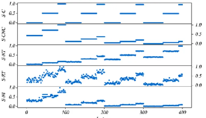
In order to select the most significant parameter to represent the network topology among (C, CNC, NT, RT, Cl), we conducted a comparison study between them. The study relies first on calculated the values of each parameter for a set of 400 projects (generated as (Attia, Dumbrava, et al., 2012)), and then investigating their sensitivity in function of topology changes. After normalised all of them over the interval [0, 1] (known as S-C, S-CNC, S-NT, S-RT, S-Cl), as shown by figure 1, we found that the S-CNC is dependent of the number of tasks, while S-C is not. For the same number of tasks, they have typically the same behaviour. And, both of them are not sensitive at all to the changes of the network topology for the same number of tasks and the same number of non-redundant relations. So we agreed with (Elmaghraby and Herroelen, 1980) (Latva-Koivisto, 2001) about the non capability of the C and CNC to efficiently measure the network topology alone. Regarding the number of generated trees “NT”, it seems to be very sensitive before standardisation, but it has a problem of order of magnitude. The returned magnitude of “NT” is exponentially grown in function of the non-redundant relations. e.g. for the group of 30 tasks, the returned minimum and maximum values are respectively (1.2E+04 and 2.4E+09) corresponding to a number of non-redundant relations of (48 and 68 relations). Moreover, for the group of 120 tasks the returned minimum and maximum values are respectively (3.5E+15 and 2.8E+34) corresponding to a number of non-redundant relations of (183 and 257 relations). This explosion in magnitude produces a high difference between the maximum and the minimum values; therefore, after standardisation it looks as insensitive. In order to accommodate this problem we calculate NT’ = log(NT), then the results was standardised as S-NT. As shown by figure 1, it looks having a very small variation compared to C, and CNC for the same number of tasks. By investigating the correlation between NT’ and CNC with the number of tasks (P-size), we found the correlation between NT’ and P-size is (Pearson correlation coefficient: PCC = 0.756) and that between CNC and P-size is: (PCC = - 0.895). This relation with the P-size translates the negative correlation between NT’ and CNC (PCC= - 0.513), shown in figure (1). Relying on this small sensitivity in NT’, it cannot be used to measure the network topology in an efficient way. Concerning Cl, it showed some sensitivity compared to CNC, and NT’, even it is highly correlated with them with respectively (PCC= 0.991, and -0.490), moreover to the correlation with the P-size (PCC= - 0.869). As we see (figure 1), the most sensitive parameter to represent the changes in network topology is the RT, where the impact of tasks number is very small. As shown, RT is
number of non-redundant relations, moreover to the changes of non-redundant relations. RT can easily dominates both NT and
Cl; i.e. - by multiplied RT with the number of tasks, the
correlation between (RTI) and NT’ is very high (PCC=
0.969), - also by only divide RT by the number of tasks the correlation between (RT/I) and Cl is very high (PCC=0. 987). Therefore, we will adopt RT to represent the project network topology. Moreover, the calculated value is often standardised over the interval [0, 1].
Figure 1 an aggregated plot of the standardised parameters of (C, CNC, NT, RT, Cl)
1.3 Network shape
The shape is a characteristic of the network, which can be distinguished relying only on its surroundings and outlines. The network shape can be specified on bases of some parameters: a measure of the network length, a measure of network width, and the measure of the relationships between the length and width (Boushaala, 2010). We added to them the measure of the network asymmetry.
1.3.1 Length and width measure
Network length: The network length is defined by (Valadares Tavares et al., 1999) as the longest path measured in terms of the network hierarchical levels. These hierarchical levels can be simply defined by considering project network as a sequence of the stages or ranks. Each stage represents a specific progression level. Network length “NS” can be considered as the maximum progressive level “NL”, this indicator can be computed as: NS = (NL-1)/(I-1). This measure is normalized over the interval of [0, 1]. With NS=0, being the completely parallel network, and NS=1 for completely serial network.
Network width: if the network length is considered aligned with the horizontal axis, then the network width is the vertical one. The network width can be defined relying on the number of activities at each stage in the network, (Valadares Tavares et al., 1999). First, the number of activities at each rank or progressive level (WL(l), with l= 1,2,…, NL) can be computed, then the rank width indicator computed as WI(l)
=(WL(l)-1)/(I-NL). The maximum width denoted by:
(
)
1WL
l
Max
MW
NL l
, can be used to signify the networkwidth.
In order to show the interaction between the length and width of the network, we adopted the aspect ratio. The aspect ratio (AR) is a dimensionless measure that can be considered as one of the common interaction between the length and width of any planer shape, images or videos. Pascue (1966) proposed it to be used as one of network (activities on arcs) complexity measure to indicate the length to breadth ratio of a given network. By considering the length of the network is equal to
the number of progressive levels NL and its width is the maximum number of tasks per level, the aspect ratio can be defined as: AR = (NS/MW : 1). As the aspect ratio increased from a datum value of one as the network become more serial and narrow, contrary is true, as the aspect ratio is less than unity as the network become more thick and short. As it will known the parallel network is more complex than serial one in scheduling, so we adopted the inverse of the aspect ratio.
1.3.2 Tasks distribution and asymmetry measure
In order to reflect the network shape relying only on the distribution of tasks along the network length “NL”, we propose to use one of the descriptive statistics such as the asymmetrical measure “skewness”. The asymmetry measure “ASyM” is a dimensionless measure of the asymmetry of data distribution around its mean. The value of the ASyM can be positive, negative, or even undefined (0.0). By interpreting the value of ASyM the distribution of tasks and so the network shape can be simply figured out. In order to standardise this measure we propose to use the logistic function, we called it the standardised asymmetry measure: SASyM =1/(1+e ASyM).
Relying on this standardised form, one can find that as the tasks concentrated at the beginning of the network as the
SASyM approaches to zero. On the other side, the value of SASyM approaches to unity when tasks are concentrated at the
end of the project. In this case we consider the project schedule is more complex, where the risk of discovering the project schedule unfeasibility can be higher than the first case, for all the constructive based schedulers.
1.3.3 Network bottleneck measure
A bottleneck is a phenomenon where the resulting performance of an entire dynamic system is limited by a single or limited number of components or resources. Generally, a facility, function, department or resource if not able to meet the demand placed upon it at the specified time, it becomes a bottleneck. As example, in production lines it can be defined as the most charged work centre, such that any lateness occurs at this workstation slow down or stop the whole production line by the same amount of time. The system performance is highly correlated to its bottlenecks and vice-versa. In supply chain network, performance keys can reveal the network bottleneck especially at the interface between its members (Stadtler, 2005). In scheduling the bottlenecks can be produced from the dependent and interdependent relations between activities. It is well known that each bottleneck has two associated phenomena; the blocking and starving. The blocking occurs before the bottleneck cause and the starving occurs after it. The degree of considering a given task as a bottleneck task in a network is determined in function of its
predecessors and successors. The network structure
bottlenecks can be formulated by considering the immediate predecessors of a given task as the blocking activities (structure blocking) and its immediate successors as the starving ones. In literature, (Johnson, 1967) proposed a measure called activity density, it relying on the number of immediate predecessors (PRi) or/and the number of immediate successor (SUi) of each activity i
I. (Boushaala, 2010) commented this measures by: they consider only the maximum difference between the predecessors and successors and neglecting all the other network characteristics, (size, shape, durations, resources…etc.). It is useful to integrate such measure with other project attributes in order to increase its sensitivity, one of this integration can be found in the measure presented by (Badiru, 1988). To increase the sensitivity of thismeasure, one can find the concept of the task degree in the context of the assembly line networks. The task degree is simply the sum of its direct predecessors and its direct successors TDi = {PRi + SUi}. By constructing the tasks’ degree vector: {TD1,TD2,…, TDI}, the maximum value:
)
(
1 max i I iTD
Max
TD
can be considered as one of thenetwork structure measures (Otto et al., 2011).
2 TEMPORAL BASED PARAMETERS
2.1 Tasks durations based parameters:
Certainly, the temporal characteristics of a project can affect the project complexity moreover the performance of a given project scheduler. The project temporal characteristics have been previously used in the analysis of the performance of the heuristic methods by (Patterson, 1976). Some temporal indicators can be used relying on activities’ durations, such as: - Sum of activities’ durations, - Average activity duration - and the variance in activity duration). In our proposed problem the exact activity duration isn’t known in advance and it depends on the productivity of the operators selected to perform it, only we have for each activity three associated values: minimum duration Di
min
, standard duration Di, and maximum duration
Dimax. In order to deal with such uncertainty, we will use the three values simultaneously to represent the nature of activities durations. Often there are some methods to estimate the activity processing duration based on the three values of (Dimin,
Di, Dimax): one of them is relying on the probability-Distribution. As stated by (Demeulemeester and Herroelen, 2002) there are some assumption: the project activities are independent regarding the duration of each one without taking into consideration the effect of resources availabilities in case of parallel task, the density function of the activity duration can be represented by the beta-distribution. Then one can approximately extract the task mean and its standard deviation based on the known (Dimin, Di, Dimax): μdi=(Dimin+4×Di+
Dimax)/6 and the variance: νdi = (Dimax-Dimin)2/36. We adopt the use of tasks’ mean durations and their standard deviations. Consequently, one can calculate the average of activities’ mean duration (ATMD=∑μdi/I), and/or the average of their standard deviation (ATSD).
2.2 Project contractual duration
The project contractual duration is a temporal convention or relationships between two or more parties (buyers and sellers) to deliver/realise a specific object/service with definite specifications and costs. Generally, there is an amount of flexibility or temporal tolerance to deliver the project also discussed between the contract parties in order to consider the changes in the working environment, if any. Any violation of the project schedule from this flexible interval, the payer parties will have extra costs such as storage costs or tardiness penalties (Vidal et al., 1999). The relative relation between the project contractual duration with respect to the project critical path length (neglecting resource constraints) can affect the project schedule complexities. We propose to consider this temporal flexibility factor in the characterisation of the project difficulties, known as project contractual duration factor “PCDF”. As previously presented, each task has three associated durations (Dimin, Di, Dimax), this indicator can be presented as in equation (3). Knowing that the value of “PCDF” is always with the interval [0, 1], if L ≤ ∑Di
max .
)
(
)
(
1
min 1 max minCP
D
CP
L
PCDF
I i i
(3)Where L is the project contractual duration, CPmin is the project critical path length considering that all tasks have their minimum durations (Dimin). The value of PCDF = 0 indicate the easiest case the (project duration is loos) but if it approaches to unity it indicates the tightness of the project contractual duration.
2.3 Temporal-Network based parameters
This category introduced the parameters that reflect in some way the integration between the project network topology and the activities durations. As well known the project float depends on the network topology, so if there is no floats, one can conclude that all civilities are critical.
According to (Davies, 1973) the density of the network is the measure of the free float under critical path conditions. The free float of activity i is the float associated with it when all jobs start as early as possible and is measure of the ability to move a job in time without affecting any other jobs. Therefore, based on the fact that the free float can absorb some delay; a correlation to measure the network density based free-float (DFF) was originally presented by (Pascoe, 1966) as shown in equation (4).
)
(
)
(
1 1 1
I i I i i i I i id
ff
d
DFF
(4)The DFF measure is always within the interval ] 0, 1], high values indicates a very small average free float, and so less flexibility in the project schedule, consequently less freedom to make sequencing decisions without causing farther resource conflicts. In our problem we estimated the floats based on task mean duration only. According to (Patterson, 1976) the average number of tasks processing free float “ATFF can be used either.
WORK CONTENT BASED PARAMETERS
2.4 Activity-resource requirement
The requests from resource can be represented by measuring the density of jobs-skills requirement matrix, considering that resources are operators with different skills. The density of this {1, 0} matrix can be measured with the Resources Factor (RF). The RF was developed by (Pascoe, 1966) to reflect the jobs-resources requirement relation, it defined as the ratio of the average number of different kinds of resources used per job to the number of the total resources required. In other words, it reflects the average portion requested of resources per each job, relying on equation (5) if RF = 1: it means each activity requires all resources for its realisation, but in case of RF = 0: it indicates that there is no resources constrained problem where no activity requires any of the resources. One of its advantages is its normalized nature over the interval [0, 1].
I i K k i,kK
I
RF
1 1 0 If Otherwise 1 01
(5)Where: Ωi,k : indicates the requirement of the activity i from the resource type k in working hours. The RF was used by (Patterson, 1976) under the name of average percent of demands for resources. In addition, it was modified by (Kolisch et al., 1995) to reflect the density of the three-dimension matrix of job-resources requirements for the
multi-mode project scheduling. (Kolisch et al., 1995) indicated that the increase of the problem RF increases the computational effort to resolve the problem, but this contradicting that found by (Alvarez-Valdes and Tamarit, 1989) where they observed that the computational effort of heuristic algorithms are influenced by the problem RF, and the problem with RF = 0.5 are more likely to have bottleneck activities which considered difficult to be scheduled than another problem with RF = 1.
2.5 Activities work content
This parameter can used to highlight the most charged resource in the firm. As the work content increases as the complexity of performing the project increased, of course for the same resources’ qualifications. The work-content per skill can be calculated as the ratio between the skill-work content to the overall project work-content. We adopted the maximum “MaxWC” and the minimum “MinWC” resource work content among all resources. Moreover, the “total work content: W” can be used as a gross measure of the total resources requirements of the project. This gross measure can be represented as a required effort per person or the required effort per working hour as a way to sizing the project.
2.6 Resources’ profile based parameters
By constructed the profile of each resource along the critical path, a set of variables can be computed such as: the maximum, minimum, average, variance of demand, moreover to the centre of profile area. But, in order to characterise a given profile, we should distinguish between two types of variables: the first is the locations variables, which represents the location of the corresponding variable relative to the project critical path, as example the location of the maximum demand or the centre of area of a given resource profile. The second type is the magnitude of variables. Therefore, we propose to measure each parameter-type separately, and introduce them in order characterise the resource-demand profile. First the resource requirement vector “RRk ” can be
computed along the critical path by: - Construct the PERT project early start and get the project duration corresponding to the critical path length “CP”. For each resource type, construct the resource-workload profile based on the previous project schedule, such that, it can be represented as a vector of resource requirement at each time period: RR = {RRk k,1,
RRk,2, RRk,3 , ..., RRk,CP},
k
K. Within literature, (Davis, 1975) presented a measure called “Product Moment”. It was used to indicate the predominant location of resource requirement with respect to time periods of project duration. Then (Kurtulus and Davis, 1982) proposed average resource loading factor. Recently it was used by (Browning and Yassine, 2009) for multi-projects scheduling problem. This factor identifies whether the bulk of a problem’s total resource requirements fall in the front or back half of its critical path duration. Also the maximum load location and magnitude was proposed by (Kurtulus and Narula, 1985), developed a project summery measure relying on the maximum consumption of a given resources and called it called the maximum load factor. As mentioned previously, we adopted the separation of the magnitude and the location. Therefore, for the location variables, we propose a dimensionless one calling it “profile central factor: PCF”, it is simply a centre of area of a given workload profile. It can be calculated based on the product moment of (Davis, 1975) as equation (6). The proposed formula calculates the central of the work-content with respectto the project start date. This measure is normalized over the project critical path length, it always located within the interval of [0, 1]. It simply signifies the point (date) on the critical path at which the required workload is exactly halved.
CP t t k CP t t k kRR
t
CP
RR
PCF
1 , 1 ,(
1
/
2
)
(6)The average value of all resource profiles can be used to indicate the project PCF. Another purely location measure can be proposed such as resource-bottleneck location “RBL”: it gives the location of the maximum required load:
)
(
1 t
CP
E
RBL
k
, where εt : is the time period at
which a maximum peak has been observed there, E○ number of observations of the maximum peak. This measure is a dimensionless that can be considered as the ratio between the locations of the bottleneck with respect to the critical path length. It is normalised over the interval [0, 1]. The value equal or near zero signifies that the resource bottleneck occurs at the project beginning and the values approaches to unity signifies its location at the project terminations stages. For a set of resources, the mean value can be used to indicate the project
resources bottleneck location:
RBL
RBL
K
K k k
/
1
.Regarding the magnitude of resources profiles, we propose to
use average resources profile factor:
ARPF=
RR
K
CP
K k CP t kt
1 1. It represents the average
daily demand along the project. Moreover, we propose to use the maximum value of each skill profile as a measure of resource bottleneck. Therefore, the average resources
bottleneck “ARB =
RR
K
K k k/
1 max
. Where, RRk max is themaximum value of the profile of the resource k. By considering the resource profile as a distribution function, the coefficient of variation can be used also, as follows:
k CP t kt k k
RR
RR
CP
RR
CV
(
)
/(
1
)
1 2 ,
(7)The coefficient of variation is simply the ratio between the standard deviation of the demand and its mean “RRk ”. The
advantage of this coefficient of variation is its dimensionless nature, and it always gives a variation degree relative to the mean. After calculating the coefficient of variation to each resource type; the mean value can be computed:
K
CV
CV
K k k
1 .Regarding the technical complexity, it can be considered as one of the parameters that affect the productivities of workforce and their experience accumulation. These rates of productivities are highly correlated to the technical complexity of the required work-content and task complexity (Osothsilp, 2002). Therefore, the number of technologies involved in the project (e.g. mechanical, electrical, hydraulic, aeronautic, digital…), and the complexity of these technologies affecting the overall project complexity. For instance, the technical complexity can be simply represented as a novelty degree of the required skills or resource types (machines, equipment,
tools, the required raw material….), i.e. simply it reflects the similarities degree between the new project work-content and that has been performed prior by the same workforce. This novelty degree can be measured relying on the ratio between the new required skills and the total skills required to create the project. The value of 0 signifies that all the required skills of work-content are previously operated, and unity value indicates that the project is completely novel. For the same worker, the technical complexity can be modelled related to the similarity degree between the actor main skill and the new required one. In the current model, we propose to integrate only the similarity degree between skills for the same project, as discussed in (Attia, Dumbrava, et al., 2012)), this similarity degree can affect the productivity levels of the workforce for their secondary skills. It was calculated as the average value of all the pairs of skills in the project, known as “SD”.
AVAILABLE RESOURCES PARAMETERS
Availability is always measured relative to the requirements, i.e. it reflects the relation between demands and availability of a given resource. The computational effort to resolve a given problem logically is a function of resources number and availability, some authors such as (Elmaghraby and Herroelen, 1980) argued that there is a bell-shaped relationship between the scheduling computational effort and the resource availability. This conjecture is then confirmed by (De Reyck
and Herroelen, 1996b) by using the
Resources-Constrainedness (RC) introduced by (Patterson, 1976). For measuring only the availability of resources regardless activates demand, for each skill a vector of real workforce can constructed to represent the set of availability workforce per time period: Ak,t. Relying on this vector, the average availability related to the project critical path length can be
estimated as:
RA
A
CP
CP t t k k
1 , . In case of constantresources per period “|Ak|”, the average availability can be
computed as: RAk Ak RAk,ttCP, then the
average real workforce can be computed as:
K
A
ARW
K k k
1.
In reasons of the heterogeneous productivities nature of the workforce in the proposed problem, moreover to the polyvalent, we propose to use the operators’ overall average productivity. As the productivity of each operator in practicing a specified skill is already normalised over the interval [0, 1], the overall mean productivity “” is also normalized over the interval [0, 1]. And it can be computed as follows:
K k k K k A a kA
K
θ
a,1
(8)Where Ak is the cardinality of the set of operators who can master the skill k. As the value “” approaches to unity it indicates that the majority of the firm’s staff are experts in practicing the specified skills, and reciprocally is true. In order to predict the available labour capacities, we propose to use this parameter as an indicator of overall capacity by integrated it with the real number of resources from each type. This available capacity can be computed by either the number of working hours, or the number of effective persons. The overall available capacity “OAC” of the staff (in equivalent number of persons) can be calculated and defined as: OAC = ×A.
ACTIVITIES- RESOURCES INTERACTION
The assessment of the interaction between project activities and resources actually can be represented as an obstruction or scarcity factor. This scarcity can be defined as the condition at which at any given time t the demand for one or more resources exceeds the supply. As explained by Pascue (1966) the resource scarcity is the main problem of resources allocation problems. An increase in network complexity or resource requirement is likely to increase the obstruction of realizing a given project. For these reasons measuring scarcity of resource is very important, thus by the following we discus some of these measures.
2.7 Resource strength (RS)
In order to quantify the relation between resources requirements and their availabilities a Resource-Strength (RS) was proposed by (Cooper, 1976). It can be defined as: the ratio between the available amounts of the resource of type k to the average requirements from this resource k per job. (Kolisch et al., 1995) stated three drawbacks of this measure: -the RS is not standardized within the interval [0, 1], - the small RS doesn’t guarantee a feasible solution, - the third is “the myopic fashion in which the scarcity of resources is calculated”. In order to overcome these three drawbacks (Kolisch et al., 1995) modified the previous correlation for the multi-mode RCPSP. Relying on these modifications, we propose to measure resources strength as equation (9). Relying on the fact that the project can be executed with the minimum resources if all tasks had been prolonged to their maximum durations and contrary is true; the project can be executed with the maximum resources consumption, if all tasks had been compressed to
their minimum durations. Therefore the minimum
requirements can be calculated based
on:
[
, max]
1 min i k i I i kMax
D
R
, such that all tasks
have their maximum durations. In order to determine the maximal per-period demand of job i from resources with skill
k, we can calculate
R
kmaxas the peak demand of resources master skill k in precedence-preserving earliest start schedule, when all tasks have their minimum durations. As a results the resources strength can be measured by the equation (9), taking into account that the maximum available capacity per-periodQk was calculated based on the French regulation considering the standard working hours per week CS0= 35 hours, and number of weekly working days NJS=5 days.
m in m ax m in k k k k k
R
R
R
Q
RS
, Where:NJS
A
Q
S k k 0C
(9)As shown by equation 9, RS gives the easiness of conducting a project not its complexity related to resources scarcity. Therefore, in order to use it as a project complexity scale, we propose to normalise it as shown by equation (10). We call the new measure as the resources scarcity index RSI: it computed relying on the average resources strength of all skills (RS ).
The new RSI is always within the interval [0, 1] whatever the resources capacity and the required workload.
1
)
1
/(
2
1
e
RSRSI
(10)2.8 Resources-Constrainedness
The resource constrainedness measure was first developed by (Patterson, 1976) to be used as resources related parameter in his investigation of the heuristic performance in function of the project specifications. As stated by (De Reyck and Herroelen, 1996b) this measuring can be considered as a pure measure of resource availability, where it isn’t incorporate information about the network. For the current resources specifications, we propose to compute it as equation (11), where,
TR
k is the task’s average requirement (in a number of working hours per day). k k k TR Q RC :
I i I i i k i kd
TR
1 0 k i, If Ot h erwise 1 0 1 ,)
(
,
k
K (11)The project complexity related on the resources
constrainedness can be estimated based on the average value
as:
RC
RC
K
K k k
1 .By integrating Resources-Constrainedness and the project temporal dimensions, we modified (Patterson, 1976) model as equation (12), such that the temporal resource constrainedness “TLCk” can measures the ratio between the average requirement work content of the task-from resource of type k to the total number of available hours during the project duration for this skill k. We developed this parameter to represent the project complexity factor as the ratio between the average number of required task-resource (in hours) to the available average workforce, and relying on the internal accordance within the firm during a pre-specified project contractual duration. We suppose that the contractual duration will be calculated based on the tasks standard durations only without taking into account the resources constraints, but there is a period of flexibility to deliver the project β can be added to the project contractual duration L. Adopting this assumption
TLCk can be shown as equation (12). The average value:
K
TRC
TRC
K k k
1can be used to indicate complexity related to all skills.
A
L
k
K
TRC
k I i I i k i k
NJS
(
)
,
C
S0 1 0 k i, If Otherwise 1 0 1 ,
(12) 2.9 Obstruction FactorThe obstruction factor is first proposed by (Davis, 1975); relying on four attributes: the network typology, temporal characteristic presented by the length of the schedule, the activities resource requirements, and the resource availability. He called it “O-factor” it is a measure of the ratio of excess resource requirements to the total work content. It calculated based on two steps: first, the O-factor should be calculated for each resource type; the second is the aggregation of all the resources factors to only one average value “OF”, as:
0
;
,
,
1 , ,A
W
k
K
RR
Max
O
k CP t t k t k k
K k kO
OF
1 (13)Where: Ok = the obstruction factor of resource type k; Ak,t = the available per period t from resource type k; RRk,t = the total requirement at period t from resources type k based on early start job scheduling using tasks mean durations; Wk = the total work content from resources type k based on early start job scheduling.
2.10 Project load density
(Davies, 1973) presented a measure relying on the integration of resource utilization and its availability during the project period. This measure integrates mainly four attributes: the resources requirements, activities durations, resources availability, and the length of the critical path (CP). He called it utilization of resource k. Aligned with this measure, we propose a measure that represents the project load density per skill, we get it as the ratio between the total workload required from a given skill to the probabilistic available standard operators’ capacity from this skill. This Project load density
PLDk can be represented by the following:
A a a k a S I i ik knk
L
NJS
PLD
1 , 0 1 ,)
(
C
For each k
K (14)Where, nka is number of skills that an operator a can master with productivity level greater than the minimum required qualifications. We propose the average value of different PLDk to represent the project load density “PLD”.
COMPOSITION OF PROJECT COMPLEXITY INDICES
From all of the previous discussed quantifiers and after selecting the most sensitive to represent each dimension of the project. We have mainly five dimensions: project network, project temporal characteristics, project work content, pure resources measures, and the weight of workload to resources. Almost all quantifiers are already normalised over the interval [0, 1] except {TDmax, ATMD, ATSD, W, ARPF, ARB, CV, and
OCW}. In order to normalise all of them, we propose to project
each of these quantifiers over the interval [0, 1] using the logistic function of their log scale: 2/(1+e-log(x))-1: where x ={TDmax, ATMD, ATSD, W/1000, ARPF, ARB, CV, OCW}. At x equals to zero the normalise value is also zero; at x approaches to a very large number the normalised value approaches to unity.
Now we propose to aggregate all of them to produce the smallest number of project complexity measures using the principal component analysis “PCA”. PCA is one of the extraction methods of factor analysis or data mining techniques that used to reduce the data into a smallest number of variables relying on the linear algebra. PCA is linearly transforms an original set of observations of possibly correlated variables into a set of values of linearly uncorrelated variables called principal components. PCA accounts for most of the variance in a set of observed variables. These smaller number dimensions are capable to represent most of the information in the original data. Where, the reduced number of uncorrelated variables is much easier to understand and use in further analyses than a larger set of correlated variables, for more details (Jolliffe, 2002). To conduct this study, let us set the data matrix Ϻ, made up of the original projects’ measures, to be a matrix Ϻ= [MI×NV] with MI the observations of project instances (the four groups of total 400 projects) and NV number of quantifiers (P_size, RT, 1/AR, SASyM, TDmax,
ATMD, ATSD, PCDF, DFF, ATFF, RF, MinWC, MaxWC, W, ARPF, PCF, ARB, RBL, CV, SD, OCW, , RSI, RC, TRC, OF,
and PLD). According to (Pallant, 2010), the applicability of
factor analysis to the data should be checked, by investigating: - the correlation matrix between variables (recommended to be greater than 0.3 between many pairs from the variables), - Bartlett's sphericity test (p_value < 0.05, here p_value = 0) - Kaiser-Meyer-Olkin measure of sampling adequacy (KMO: should be greater than 0.6, here KMO = 0.760), for more details see (Jolliffe, 2002). Therefore, the adequacy of using
PCA to the current data was approved.
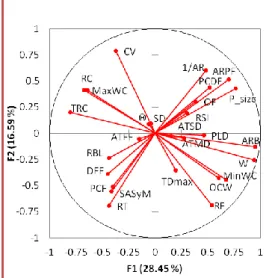
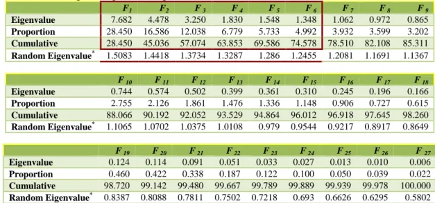
By employing the PCA analysis (using XLSTAT addinsoft), a set of factors can be obtained as shown in figure (2) of maximum size [1× NV]=[F1, F2 … F27]. The analysis is conducted based on the correlation matrix to avoid the problems related to the data scales (even we normalised all quantifiers). As results, each element within these factors has a specified rank (eigenvalue) indicates its contribution to explain the total variances in the original data i.e. the factors arranged according to their contribution in explaining the original data variances such that the first factor is the greatest one and the last is the smallest. As indicated in figure (2), and table 1, the first factor is capable to explain about 28.45% of the total variance, and the second one is capable to explain about 16.586%, etc. Each factor is loaded from all the quantifiers according to a specified contribution, as shown by figure (3), by projecting the variable to the factor axe. The quantifiers that had the highest projection cosine are those whose contributions are highest in building the axes. Nevertheless, the question is how many components should be taken into account?
To determine the number of components (Franklin et al., 1995) and (Pallant, 2010) appreciated the use of parallel analysis. Parallel analysis involves of comparing the magnitude of factors’ “eigenvalues” with those obtained from a randomly generated data set of the same size. If the “eigenvalue” of the principal factor is greater than that of random data we accept the corresponding factor, otherwise we reject it. In order to calculate these “eigenvalues” based random data, we used a software called “Monte Carlo PCA for parallel analysis” developed by (Watkins, 2000). The results shown in table 1 indicate that only the first six factors “F1, ..., F6” could be
accepted which they have “eigenvalues” greater than those were generated randomly. These six factors explained about 74.578% of the total variance in the original data.
Figure 2 Scree plot of the different Eigenvalues
Figure 3 Contributions of quantifiers on the axis of F1, and F2 Relying on these results, the rotation of axes using “Varimax rotation” was carried after identified the number of composite factors to be only six principal components “PC1, ..., PC6”. These new components were built out from the projection of the different quantifiers to the principal component axis after “Varimax” rotation, see (Pallant, 2010). The loading of different components relying on quantifiers showed in table 2, simply it represents the correlation between each principle component and the quantifier after the rotation. The quantifiers that had the highest projection square cosine on axes after rotation are those whose contributions are highest in building the principal component. Therefore, we find high correlation between these quantifiers and the principal components. In order to understand the composition of the new principal components, we performed a hierarchical clustering of all quantifiers as shown by figure 4. This cluster analysis grouped the similar variables in clusters. At level of similarity = 0.30, we found ten clusters.
Figure 4 the hierarchical cluster analysis of quantifiers Based on factor loading, squared cosines and cluster analysis, we can identify and understand the elements of each principle component and get their scores from table 2. By the following, we discuss the construction of each principal component:
- The first principal component “PC1” contains two clusters
(cluster #2, and #10). The cluster #2 contains some of resources, workload, and resources bottleneck variables, so it can represent the project sizing. These variables in somewhat are similar, where as the workload increased the required resources increased, and so the magnitude of project resources bottleneck. The other cluster #10, contains constraindness per task “RC” and that of the project “TRC”, moreover to the maximum requirements per skill and the variation in resources