Faculté des Sciences Appliquées
Département d’Architecture, Géologie, Environnement et Constructions Jean-Marc FRANSSEN, professeur ordinaire
Liege, July the 15th, 2016
Tensile membrane action
Expert judgement about
the Bailey-Moore simple method and the software MACS+
2
nddraft
Jean-Marc Franssen
Foreword : this document is a genuine report of the work that we performed, based on our most recent knowledge and with the best of our ability, free of any pressure from any kind. No result obtained has been concealed.
Secteur Ingénierie Structurale (SE) / Ingénierie du feu
Quartier Polytech 1, Allée de la Découverte 9 (Bât. B52/3) 4000 Liège (Belgique) Tél. ++ 32 (04) 366 92 65 Email: [email protected]
This report is the second version presenting the results of our analysis of the Bailey-Moor simple method. Compared to the first version dated October 28, 2018:
Some editorial and typing errors have been corrected.
New geometries have been studied (6 x 6, 6 x 12, 9 x 12 and 9 x 15 m²).
All simulations of SAFIR have been run with all variables of the concrete model in Double Precision
The displacement criteria is evaluated from the initial configuration.
Any reference to the version 2.0.6 of the software MACS+ has been delete as it is now obsolete. Only version 3.0.1 and 3.0.2 are discussed here.
A mesh sensitivity has been added (2.2.2)
Table of content
1
The Bailey-Moore method ... 4
1.1 General overview ... 4
1.2 Detailed developments ... 8
1.2.1 Estimation of the membrane forces ... 8
1.2.2 The enhancement factor ... 10
1.2.3 Estimation of the displacement ... 15
1.2.4 Contribution of the unprotected beams ... 15
1.3 The FRACOF method ... 16
2
Numerical simulations ... 20
2.1 Thermal simulations ... 20
2.1.1 Model of the composite slab... 20
2.1.2 Model of the steel beams ... 23
2.1.3 Some results ... 25 2.2 Mechanical simulations ... 26 2.2.1 The model ... 26 2.2.2 Mesh sensitivity ... 28 2.2.3 7,5 x 15 m² ... 30 2.2.4 9 m x 9 m ... 36 2.2.5 6 m x 6 m ... 39 2.2.6 6 m x 12 m ... 40 2.2.7 9 m x 12 m ... 41 2.2.8 9 m x 15 m ... 43
2.2.9 3 sides heating versus 4 sides heating ... 44
2.2.10 Influence of lack of overlap ... 46
2.2.11 Effect of a localized fire ... 49
3
Conclusions ... 53
3.1 Tensile membrane action ... 53
3.2 The Bailey-Moore simple method ... 53
3.4 Numerical modelling ... 55
4
Bibliography ... 56
5
Annex: problems in the Bailey Moore simple calculation method ... 57
1 The Bailey-Moore method
1.1 General overview
In this section, we present the main features and assumptions of the Bailey-Moore simple calculation method. This method is used to calculate the fire resistance with respect to the load bearing capacity performance R for floor slabs loaded by uniformly distributed vertical loads.
On the base of this method is the experimental observation that failure in the fire situation does not occur until very large displacements develop. At this ultimate stage, the failure mechanism is not anymore the “classical” yield lines mode where portions of the slab, assumed to be rigid, turn with respect to each other along linear yield lines in which only bending moments are present (no axial force) , see Figure 11.
At the ultimate stage in the fire situation, the deflection shows a double curvature shape, with both curvatures in the same direction and the radius of curvature varying continuously in the plane of the slab, see Figure 2.
1 The four plates defined by the yield lines will be called here “the two trapezoidal plates” and “the two triangular
plates”.
Figure 2: deflection calculated numerically
The central part of the slab behaves like a piece of fabric, a membrane, and is subjected essentially to “radial” tensile forces, while the external ring of the slab, near the vertical supports (that must be present on all 4 sides), is subjected to circumferential compression, see Figure 3. This behavior is only possible because;
1) tension in the central part of the slab is supported by a multidirectional continuous steel mesh; 2) compression in the external ring is supported by the reinforced concrete slab and;
3) the central part is anchored in the external ring.
Figure 3: membrane forces in 1/4 of a slab panel after 104 minutes of fire
Nevertheless, the authors of the simple method take the deformed shape of the yield line theory and the ultimate load capacity calculated according to this theory as a starting point of their method. From there, they improve, they “enhance” in their terminology, the calculation of the ultimate
X Y
Z
1,0 E+00 m
Diamond 2012.a.0 for S AFIR
FILE: oli_nu NODES: 1023 BEAMS: 60 TRUSSES: 0 SHELLS: 900 SOILS: 0 SOLIDS: 0 DISPLACEMENT PLOT ( x 1) TIME: 2042,027 sec X Y Z
Diamond 2012.a.0 for SAFIR
FILE: 11A433x NODES: 450 BEAMS: 24 TRUSSES: 0 SHELLS: 384 SOILS: 0 SOLIDS: 0 BEAMS PLOT SHELLS PLOT
Structure Not Displaced selected N1-N2 MEMBRANE FORCE PLOT
TIME: 6811,211 sec - Membrane Force + Membrane Force
load bearing capacity taking into account the fact that tension/compression forces exist in these yield lines.
The development of the simple calculation method is schematically described hereafter. 1. Establish a method that takes into account the effect of membrane forces at room temperature,
at least if the displacement at failure is known.
1.1. Make a hypothesis about the kinematic of the slab when it deforms until failure: the slab deforms as it would if there is no membrane force, i.e. in the same manner as the one predicted by the bending yield line theory, see Figure 1.
1.2. Make a hypothesis about the shape of the membrane force diagrams along the yield lines: membrane forces vary linearly along the yield lines, see Erreur ! Source du renvoi
introuvable. in which membrane forces are drawn only for the upper trapezoidal plate.
1.3. Make the hypothesis that the force is the same in the three yield lines at the point where they meet2, see point A on Figure 4.
1.4. From the equilibrium of the in-plane forces acting along the yield lines of the trapezoidal plate (as seen on Figure 4), calculate the relative amplitude of the membrane forces in the corners of the slab and at the intersection of the yield lines. At this stage, neither the failure load nor the amplitude of the membrane forces or of the displacements at failure is known.
1.5. Increase the membrane forces proportionally in the slab until they exceed some failure criteria, either tension in some re-bars or compression in the corners of the slab. Now, the amplitude of the membrane forces at failure is known, but not the failure load and not the displacement at failure.
1.6. Another equilibrium equation (moment of the membrane forces on the edges of half the trapezoidal plate about point E, see Figure 6) allows calculating the failure load of the slab, taking into account two favorable effects:
2 This fact was already present in the very early papers of Hayes and it is not discussed anymore in the subsequent
literature. As we have not been able to find a justification for that based on principles of structural mechanics, we assume that it is a hypothesis.
Compression Compression
Tension
A A
E
1.6.1. The fact that compressive membrane forces increase the resistance of the slab in bending around the yield lines3 and;
1.6.2. The fact that membrane forces have a lever arm with respect to the supports, which reduces the demand in term of bending resistance along the yield lines.
Both effects depend on the amplitude of the membrane forces. The first one does not depend on the displacement w of the slab but the second one is proportional to this displacement. At this stage, the failure load P and the displacement w are not known but we have a linear relationship between both:
P = a + b w (1)
where a and b are known positive constants. The failure load is thus bigger if larger displacements develop at failure.
In the terminology of the Bailey-Moore method, the failure load of the slab is expressed as an “enhanced” capacity compared with the failure load calculated on the base of the yield line theory P0, i.e. when the membrane forces are not taken into account.
P = e P0 (2)
where e is the enhancement factor.
1.7. In fact, the enhancement factor is not calculated for the slab as a whole. Two enhancement factors e1 and e2 are calculated for the trapezoidal plates and for the triangular plates respectively. The two factors are then combined into one by the following equation:
e = e1 + (e2 – e1) / ( 1 + 2 µ r²) (3)
where r is the aspect ratio of the slab (L/l) and µ is the ratio of the moment capacity of the slab in orthogonal directions.
2. Extend this method to the fire situation.
2.1. Reduce the material properties of the steel re-bars depending on their temperature. The material properties influence the constants a and b that are present in equation 1.
2.2. Estimate the displacement at failure w, which will allow calculating the failure load from equation 1. This displacement is made of two components:
2.2.1. One from the thermal bowing due to the thermal gradient that appears on the thickness of the slab. The thermal curvature is estimated based on the short span of the slab. 2.2.2. One from the strain in the re-bars, assumed to be stressed at half the room temperature
yield strength. This displacement is based on a parabolic deformed shape in the direction of the long span (but it is limited to 1/30 of the short span).
2.3. Tune4 a little bit the estimation of the displacement to better correspond to the values that have been observed in full scale experimental tests made in Cardington.
3. Add to the load bearing capacity of the slab a term taking into account the effect of the internal unprotected steel beams. The bending resistance of these beams is considered.
3 And, simultaneously, tensile forces in other parts of the slab reduce the bending strength.
4 The displacement has been tuned during the development of the method. Designers don’t have to tune their
More details about the development of the method and the hypotheses that are being used are given in the following section.
1.2 Detailed developments
1.2.1 Estimation of the membrane forces
As rigid body turn with respect to each other along linear hinges, the hypothesis of rectangular compression stress block leads to the fact that the axial force perpendicular to a yield line varies linearly with the position of the neutral axis, see Figure 5, and, hence, varies linearly along the yield line, see Figure 4.
Note: this is correct, as long as;
1. The neutral axis does not extend below the steel bar. If this occurs, there is a sudden variation of the compressive force. This situation could be present at the ends of the yield lines that end at the corner of the slab (that we will call “the corner lines”), where compression is the highest. 2. The neutral axis does not move up out of the section. If this occurs, there is no compressive stress and the tensile force becomes constant. This situation could be present in the central yield line (shown horizontally on Figure 4) and in some parts of the corner lines (near the central lines, point A on Figure 4).
A relationship is then derived between the compressive resultant in the corner lines, the tensile resultant in the corner lines and the tensile resultant in the central line. This relationship comes from two equations of equilibrium of the rigid part shown on Figure 4.
In these equations, the resistance in tension of the steel reinforcing mesh per unit width is TO in the direction parallel to the long edges of the slab and K TO in the direction parallel to the short edges. The resistance in bending per unit width is M in the direction parallel to the long edges of the slab and µ M in the direction parallel to the short edges.
Note: in these two equations, the authors of the simple method consider that the resultant forces are horizontal. This must be the case for the tensile resultant in the central line (for symmetry reasons). This is not so clear for the tensile and compressive resultants on the corner lines. Nevertheless, these resultants are close to horizontal if the displacements of the plates are small with respect to the dimensions of the slab.
Co m p ressi o n stre ss bl o ck Tensile force Neutral axis
When the resultant forces are calculated as a function of the maximum forces that exist at the extremities of the corner lines, the expression mentioned previously allows computing a parameter k which is the ratio between the compressive membrane force in the corner lines (i.e., at the corners of the slab) and the tensile force at the other extremity of the corner lines (points A on Figure 4).
The next step is the derivation of the maximum tensile force at this extremity of the corner line where it meets the central line. Two possibilities are considered, each one associated with a failure mode.
1) The first failure mode is a tensile crack in the center of the slab, parallel to the short edge of the slab (line EF on Figure 6). It is assumed that this crack extends from one to the other longitudinal edge of the slab, which implies that the compressive zone near the long end of the slab (point E) has a width that is infinitely small. The tensile force along the crack is calculated assuming that all the reinforcement along the section is at ultimate tensile strength.
The equilibrium of moment of the resultants with respect to point E yields the parameter
b which defines the tensile force at point A. Notes:
1) In the equilibrium of moment mentioned above, the shear force S along the corner line is taken into account. The value of this shear force is calculated from horizontal equilibrium of the triangular plates, see Figure 7.
2) If the horizontal component of the shear force and the horizontal component of membrane forces are in equilibrium on the corner line in the triangular plate, see Figure 7, they are also in equilibrium in half the plate of Figure 6. As a consequence, the plate shown on Figure 6 is in horizontal equilibrium only if the compressive force that is concentrated on point E is equal to the horizontal tensile force on line EF.
F
Figure 6: membrane forces in failure mode 1
E Tension
Compression
Tension A
2) The second failure mode is compressive failure of concrete in the corners of the slab. The total compressive force in the section is the addition of:
a. the compressive membrane force that can be seen on Figure 4 and b. the compressive force due to the bending along the yield line.
The total of these two forces cannot yield a compressive stress that exceed 0,85 x fck calculated on the hypothesis that the maximum stress-block depth is equal to 0,45 d. This value of 0,45 is a very strong hypothesis that the authors of the method don’t justify.
The fact that two different enhancement factors are obtained for the trapezoidal and the triangular plates would be due, according to Tony Gillies, to the fact that the vertical shear component between the trapezoidal and the triangular plates (i.e. in the corner yield lines) has been neglected in the equilibrium equations.
1.2.2 The enhancement factor
Now, assuming that we have all membrane forces inside the element and that they are correctly evaluated, here are some thoughts about the enhancement factors.
We will use a uniaxial element, in order to simplify the discussion. We assume that the element is supporting a UDL of value p. The span is L.
1) Simply supported beam, no axial force, no large displacement
Acting bending moment at mid spa: M = pL²/8 Acting axial force: N = 0
Bending capacity of the section: Mpl = Wpl fy The ultimate load is given by p0 = 8 Mpl / L²
This corresponds to Eq. (5.2) in the ECCS publication.
This is called the reference plastic load. This is the one that we have to enhance.
2) Simply supported beam, with an axial force, no large displacement
Let us assume now that, for any reason, the central part of the beam is subjected to a compressive force Fc in addition to the applied vertical loads. There is still no large displacement considered.
Acting bending moment at mid spa: M = pL²/8 Acting axial force: N = Fc
If the section is made of reinforced concrete, the compressive axial force will increase the resisting bending capacity of the section, Figure 9, see Eq. (5.34) in ECCS publication.
The ultimate value of p is now given by:
P = 8 Mpl,N / L²
If we note e2 the ratio Mpl,N/Mpl, we can write p = e2 p0
Note that, if the axial force is tension, e2 could be smaller than 1. It is then amazing that the overall factor e2 calculated for the biaxial slab panel treated by the Bailey-Moore method is greater than one, since most of the member is subjected to tensile forces. In fact, as there is no horizontal force applied on the slab panel as a whole, tensile and compressive forces equilibrate each other in the slab panel and, indeed, application examples carried out systematically yield a value of e2 that is very close to 1,0.
Fc Fc M N Mpl Mpl,N
3) Deformed beam with an axial force, no enhancement of the plastic resistance
Let us assume now that the beam is still supporting vertical loads but is also subjected to large displacement of amplitude w and a tension horizontal reaction Ft, see Figure 10. Let us assume also that the section is such that the bending resistance is not influenced by the axial force. This may happen, for example, if the section is made of steel and the axial force is small.
Acting bending moment at mid spa: M = pL²/8 – Ft w Acting axial force: N = - Ft
The ultimate value of p is now given by: p = 8 (Mpl + Ft w) / L² If we note Ft w / Mpl = e1, we can write p = p0 (1+e1)
We see that e1 is proportional to the displacement w.
Note that, in a uniaxial element that deflects downward, we need a tensile reaction force at the support to decrease the bending moment at mid span. In a biaxial element, we have tension in the center as well as compression forces near the supports which are in self equilibrium.
It is somehow amazing to note that the moment produced by the axial forces is evaluated in the Bayley-Moore method, for each rigid plate, with respect to the supports.
Indeed, the effects of actions (bending moment and axial force) must be evaluated and checked, normally in any section, practically in the most critical section(s), here along the yield lines and not along the supports where no effect of action is present.
For example, in the uniaxial situation like the one shown in Figure 10, the critical section is section A located at mid span. The effects of action (MA, NA, VA) can be easily calculated from the equilibrium of half a section, see Figure 11, assuming that we know the value of the horizontal reaction FtB (the uniformly distributed load p has not been represented on this figure for clarity reasons).
The shear force VA is equal to 0, because the vertical reaction RB balances exactly the vertical load pL/2 applied on this substructure.
The axial force NA, that we will call here FtA is exactly equal to the horizontal reaction FtB from the equilibrium in the horizontal direction.
The bending moment MA has contributions from the vertical forces and a contribution from horizontal forces.
MA = MA(vertical forces) + MA(horizontal forces)
w
Ft Ft
A B
= [ pL/2 x L/2 – pL/2 x L/4 ] - FtB x wA = pL²/8 – FtB x wA
Whe can nevertheless verify that the same result is obtained for the contribution of the horizontal forces if the moment is evaluated with respect to the support, point B, see Figure 11. Indeed:
MB = FtA x wB = MA = FtB x wA Because FtA = F
tB and wB = wA
Figure 11: half of the uniaxial member with a horizontal force
It can to be noted that the same equivalence holds for vertical forces because the moment of vertical forces with respect to point B is pL/2 x 0 + pL/2 x L/4 = pL²/8
This is because of a principle of structural mechanics: when a group of forces is in equilibrium in translation, if they produce a certain moment with respect to a point in the plane, they produce the same moment with respect to any point in the plane.
In the biaxial situation that prevails in a slab panel, the critical sections are along the yield lines. The same principle can be generalized: when a group of forces is in equilibrium in translation, if they produce a certain moment with respect to an axis in space, they produce the same moment with respect to any parallel axis in space.
For the trapezoidal plates such as the one shown on Figure 12, taking the moments produced by membrane forces S, T1, T2 and C with respect to the axis B on the support is thus equivalent to evaluating the moments with respect to the central yield line A because these forces are in equilibrium in translation. In the simple method, this contribution is divided by the plastic capacity of the slab Mpl (in Nm/m) multiplied, not by the length of this yield line but by the length of the slab in the longest direction L. Maybe is this to account for the projection of the bending capacity of the slab in the two corner yield lines on the central yield line.
wA FtA FtB
A B
Figure 12: bending moment with respect to the support
wB R MA T1 T2 T2 C C A B S S
For the contribution of membrane forces to the reduction of bending moments in the corner lines of the triangular plates, the moment produced by membrane forces S, T2 and C is also evaluated with respect to the support (now on the short side) and also compared with the plastic capacity in the slab, multiplied now by the length of the short side.
4) Deformed beam with an axial force and enhancement of the plastic resistance
We add now the two effects mentioned under point 2 and 3.
We have a horizontal reaction near the supports that will decrease the bending moment at mid span (in a biaxial situation, this would be produced by the anchorage of the steel mesh in the outer compression ring). Let us assume that, from the particular statics of bi-axial members, we have at the same time compressive axial forces at mid span that increase the bending strength of the section5.
We have now the equation: p L² / 8 – Ft w =Mpl,N
or, (p L² / 8) / Mpl = e1 + e2
and finally: p = p0 (e1(w) + e2)
which is Eq. (5.49) of the ECCS publication.
This simple reasoning explains why the two enhancement effects really add to each other whereas intuition would lead to multiply two enhancement factors.
The fact that the two enhancement factors must be added and that the sum multiplies the yield line ultimate load, see the equation above, can also be accepted more easily when one notes that, if the enhancement is small, e1 tends toward 0 and e2 tends toward 1.
5 If the force is tension, it will decrease the bending resistance
w Ft Ft A B Fc Fc
1.2.3 Estimation of the displacement
The displacement in the center of the slab is a key parameter of the method because it influences strongly the enhancement factor. This displacement must be estimated.
In the simple method, this displacement is made of two components: one due to thermal bowing assumed to be given by a circular deformed shape and one due to elongation of the bars from applied stresses assumed to be given by a parabolic shape.
The fact that both shapes are different is not an issue if the displacements can be added. The fact that the thermal bowing is calculated based on the short span whereas the mechanical displacement is based on the long span may lead to think of a system where two elements are working in parallel (more or less as one beam across the short span and another beam across the long span, both having the same displacement in the center of the slab) and their respective displacements are added. In fact, the model does not say so. The model admits that there is a thermal displacement and a mechanical displacement in each direction. More difficult to explain are the facts that:
1) Each displacement is evaluated based on a uniaxial behavior, as if there is no effect from the other direction.
2) The thermal displacement is based on the short span (probably the best choice if it has been decided to consider a uniaxial behavior) but the mechanical displacement is based on the long span whereas consideration of the short span is expected to give the true behavior if the aspect ratio (long span/short span) tends to high values.
3) These continuously derivable shapes considered here are totally incompatible with the multilinear shapes considered in the yield line theory which is at the base of the method, see Figure 13.
1.2.4 Contribution of the unprotected beams
In the simple method, the load bearing capacity of the unprotected beams is taken as the bending capacity of the composite beams made of the unprotected steel profiles collaborating with the concrete slab. This means that the upper part of the concrete slab is assumed to work here in compression at mid span of the beams, i.e. in the center of the slab where, for the evaluation of the membrane forces, the slab is assumed to be fully cracked in tension. This is a severe contradiction.
²
≠
Short span
≠
Long span
The contribution of the unprotected steel beams to the loadbearing capacity is particularly significant during the first 30 minutes of the fire and decreases thereafter with the elevation of temperature in the unprotected steel sections. The contribution of the unprotected steel beams may nevertheless still account to around 15% of the contribution of the slab, even after 2 hours of ISO fire.
1.3 The FRACOF method
The method has first been evaluated from its implementation in the software MACS+, version 3.0.1, August 2013.
The input data can be given in a user friendly graphical interface. This interface can be set to have the text in 16 different languages.
If the user tries to introduce any value that is beyond the field of application of the software, it is impossible to proceed further. The user is forced to change the value to continue the input of data. Once entered in the graphic interface, the input data can be saved in a file with extension “.frc”. This file is a text file organized according to an XML format and can thus be opened by a text editor. A series of input files can thus also be generated by any convenient mean, for example to run parametric analyses.
As far as we could observe, the software is quite robust (it does not crash during execution or from any action of the user) and the implementation of the Bailey-Moore method is correct6.
It is also quite easy to use. It has been verified, for example, that there is a sketch showing the definition of the longitudinal mesh area as opposed to the transverse mesh area. The sketch is in the screen “Slab”, see Figure 14. The longitudinal bars are parallel to the span 1, i.e. parallel to the internal unprotected beams.
Figure 14: orientation of the mesh
The reinforcement mesh is assumed to be made of cold-formed steel (private communication). Since version 3.01, it is possible to consider flat slabs (in addition to corrugated slabs).
Limitations of the software:
It is not possible to evaluate the fire resistance of a slab panel that has no unprotected beam. At least one unprotected beam must be present. This is yet not surprising as the aim of the software is to check the stability of slab panels with internal unprotected beams. It is nevertheless still possible to approach the solution with no unprotected beams by introducing a single beam with a minimal section and minimal yield strength.
The beams that form the slab panel must be based on hot rolled steel profiles, either used as such or in the form of cellular beams (beams with large web openings), either based on European, UK, or American sections. It is not possible to define user (welded) sections.
European sections must be of the IPE type.
Other limitations apply, normally conforming to common sense and documented in the ECCS publication and/or in the contextual help of the software. The contextual help comes in the form of short text appearing in a window called “messages”, depending on the position of the cursor in the input boxes.
In addition to a list of input data, the results produced in the report are, at a constant time step that varies between 1 and 10 minutes depending on the requested fire duration, see Figure 15:
The temperatures of the unprotected beam, of the mesh, at the top and at the bottom of the slab (the software does not warn if the insulation criteria I is lost on top of the slab);
The beam capacity in kN/m², decreasing as a function of time as the temperature in the beam increases;
A deflection that is, unduly in our opinion, called “maximum allowable deflection”. We rather consider this value, w in the theory, as an intermediate result, a parameter that is evaluated to lead to the final result. This value usually increases as a function of time;
The ultimate load bearing capacity of the slab according to the yield line theory (without enhancement owing to membrane effects). This value reduces as a function of time as the temperature of the mesh increases;
The enhancement factor. It typically increases first because of the rapid increase of the displacement but may decrease slightly later when the displacement has reached a constant value;
The slab capacity taking into account the enhancement factor (product of the two previous values);
The total capacity, sum of the beam capacity and the slab capacity;
The unity factor, ratio between the applied load and the total capacity. The fire resistance time is met when this factor is 1.
The software does not give information about the contribution of both components of the enhancement factor e1 and e2. There is also no information about the failure mode, by tension in the steel mesh or by compression in the concrete slab.
We have not seen how it could be possible to save in a pdf file the report that contains the data and the results.
Figure 15: results produced by MACS+
The load has to be introduced by the values of the leading variable action, the accompanying variable action, the dead load including beam (excluding slab) and the slab weight including mesh (this one can be automatically calculated by the software based on the steel sheet dimensions or can be entered by the user). The partial safety factors in the fire situation must also be entered for the leading variable action of for the other variable action. The partial safety factor for permanent action is fixed to 1. The design load in case of fire that results from these values is given in the report. It can be verified on Figure 16, for example, that (1,25 + 2,825) x 1,0 + 5 x 0,5 = 6,575 kN/m² has been correctly applied (we introduced the slab weight directly).
Figure 16: input of loads (correct)
Yet, for other cases, we get erratic results, see Figure 17. This was due to the utilization of a coma instead of a decimal point as a decimal separator. As shown by the difference in maximum unity factor and in the message (“ Floor slab adequate” or “Floor slab fails”), the software really considers the factored load that appears in the summary output to check the stability of the composite slab. If this value is wrong because of the utilization of the wrong decimal separator, the result of the calculation will be wrong.
After we mentioned this to CTICM, we received by private e-mail dated 16/11/2015 the version 3.0.2 of MACS in which this problem has been solved. Nevertheless, on 30/05/2016, version available for download on the web site of ArcelorMittal was still version 3.0.1.
We did not check the effects of using a wrong decimal separator in other entries of the software.
2 Numerical simulations
According to the request of CERIB, the method that will be analyzed here is Bailey-Moore simple method applied to composite floors based on trapezoidal or reentrant cold formed steel decks. The composite floor is supported by steel beams with at least one unprotected steel beam in a slab panel. The floor acts in a composite manner with the steel beams.
The simple method is evaluated by its implementation in the software MACS+ developed by CTICM and ArcelorMittal. It is evaluated by comparison with results obtained by the general calculation model.
The numerical analyses have been performed by the software SAFIR®, version 2016.b.1. In the numerical simulations, a physical reason was found at the end of nearly all runs, either a vertical asymptote in the displacement curve, or steel entering in the descending branch in either the steel beam or at least one shell finite element.
2.1 Thermal simulations
Only the ISO 834 fire curve is considered in this analysis.
2.1.1 Model of the composite slab
Thermal properties of concrete are from the Eurocodes, with specific mass of 2300 kg/m³, water content of 46 kg/m³ (2%), coefficient of convection on exposed surface of 25 W/m²K, coefficient of convection on unexposed surfaces of 4 W/m²K, emissivity of 0,7 and thermal conductivity equal to the average between lower limit and upper limit as defined in clause 3.3.3 (2) of EN 1992-1-2.
As the shell finite element of SAFIR is a flat element, the section of the composite floor is simplified. The presence of the steel deck is not taken into account, neither in the thermal nor in the structural analyses (this hypothesis is also taken into account in MACS+).
The concrete slab located above the steel deck is modeled with its exact depth while the ribs of the slab are modeled by a smeared uniform layer of concrete (this protective layer will have no load bearing capacity in the structural analysis).
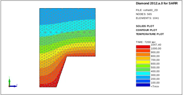
In order to choose the appropriate value for the thickness of the protective layer, a model has first been made of a real 2D section. We modeled in SAFIR the COFRA+60 composite slab. The steel deck is not modelled and no shadow effect is considered. We can see that the temperature at the level of the mesh is not uniform, see Figure 18.
Figure 18: isotherms after 120 minutes
We noted the evolution of the temperature at the level of the steel mesh for 3 points in the model of Figure 18: extreme left, extreme right and intermediate position. This evolution is shown in Figure 19 together with the temperature evolution given by MACS+. It can be seen that MACS+ follows more or less the temperature calculated by SAFIR for the intermediate position7 during 30 minutes and is closer to the maximum temperature thereafter. The hypothesis used in MACS+ thus seems to be reasonable, even slightly on the safe side compared to the results given by SAFIR.
Figure 19: evolution of the temperature in the steel mesh
7 This temperature can be assimilated to the average temperature in the steel mesh.
X Y
Z
Diamond 2012.a.0 for SAFIR
FILE: cofra60_2D NODE S: 565 ELE MENT S: 1041
SOLIDS PLOT CONTOUR PLOT TEMPE RATURE P LOT
TIME : 7200 sec 1047,40 1000,00 900,00 800,00 700,00 600,00 500,00 400,00 300,00 200,00 100,00 <Tmin 0 50 100 150 200 250 300 350 400 450 500 0 20 40 60 80 100 120 SAFIR 2D a SAFIR 2D b MACS mesh SAFIR 2D c
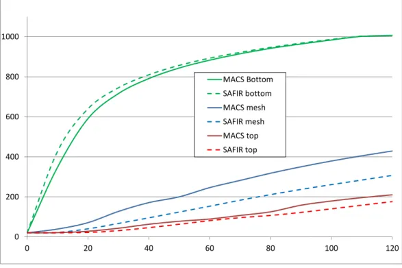
In order to derive the thickness of the protective layer for the flat slab model, equation D.15 of EN 1994-1-2 was first used. We considered a COFRA+ 60 section with 90 mm of concrete on top; equation D.15 gives an equivalent thickness of the slab equal to 23 mm; we thus made a flat slab model with a total thickness equal to 113 mm. There is not a very good fit between SAFIR and MACS+ for the temperatures at the level of the mesh, see Figure 20. It has to be noted that equation D.15 has been derived to yield good fit with the temperature on the unexposed side of the composite floor, with the Insulation criteria I in mind, see how the curves “MACS top” and “SAFIR top” compare well on Figure 20.
Figure 20: comparison between SAFIR 1D and MACS+ in a COFRA+ 60 with 23 mm protective layer
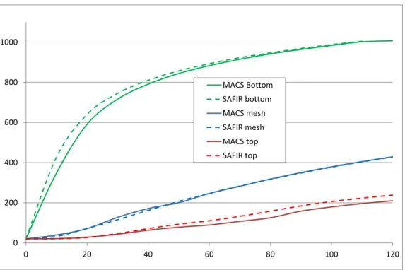
Yet, in tensile membrane action, the temperature on the unexposed side is not likely to dominate the failure mode. The temperature at the level of the mesh is more likely to be the relevant parameter. This is why different models have been created until a good fit is observed with the temperature at the level of the mesh supposed to be located at mid-depth of the concrete layer, i.e. 45 mm above the steel deck and 45 mm below the surface of the concrete slab. A protective layer of 5 mm was finally chosen. Figure 21 shows the good comparison obtained at the level of the mesh as well as on the exposed side of the slab. The temperatures on the unexposed side are overestimated by 30°C after 60 minutes while still remaining so low that this should not affect the failure mode by compression in the concrete.
0 200 400 600 800 1000 0 20 40 60 80 100 120 MACS Bottom SAFIR bottom MACS mesh SAFIR mesh MACS top SAFIR top
Figure 21: comparison between SAFIR 1D and MACS+ in a COFRA+ 60 with 5 mm protective layer
As a conclusion of this section, we note that:
1) MACS+ seems to give a correct (slightly on the safe side) estimation of the temperature in the steel mesh compared to the results of a SAFIR 2D numerical model.
2) When a flat slab is used with an equivalent horizontal layer of concrete representing the protective effect of the ribs, it is better in the numerical model to reduce the thickness of this layer compared to the value given by equation D.15 of EN 1994-1-2 if a correct evaluation of the temperature at the level of the steel mesh is the objective.
2.1.2 Model of the steel beams
The steel beam has the upper flange somehow protected by the composite slab. Nevertheless, as the proportion of the upper flange covered by the steel deck is less than 90% (when the deck is a COFRA+ 60), the steel profile is heated on 4 sides in the simulations.
For IPE 360, the coefficient of convection and the emissivity of steel are multiplied by the factor 0,9 x 2 x (0,36 + 0,17) / 1,353 = 0,705 in order to introduce in the numerical model the shadow effect8.
Coefficient of convection; 0,705 x 25 = 17,63
Emissivity: 0,705 x 0,7 = 0,4935
For IPE 600, for example, the coefficients are multiplied by 0,9 x 2 x (0,60 + 0,22) / 2,015 = 0,733 Coefficient of convection; 0,733 x 25 = 18,33
Emissivity: 0,733 x 0,7 = 0,5131
Figure 22 shows the evolution in two steel beams, IPE360 in blue and IPE600 in red, as calculated by SAFIR (minimum and maximum temperature in the section) and by MACS+ (results given every 10 8 See EN 1993-1-2 0 200 400 600 800 1000 0 20 40 60 80 100 120 MACS Bottom SAFIR bottom MACS mesh SAFIR mesh MACS top SAFIR top
minutes). It can be seen that the temperatures are slightly lower in MACS+ during the first 15 minutes but this is not considered to be a serious issue because no slab panel is designed for a 15 minutes resistance time. Between 15 and 30 minutes, the temperatures calculated by MACS are between the minimum and the maximum value given by SAFIR. Beyond 30 minutes, the temperatures calculated by MACS+ rather correspond to the maximum values calculated by SAFIR, with little differences between all values because steel temperatures tend toward the values of the ISO curve.
Figure 22: Evolution of the temperature in steel beams
As a conclusion of this section, we consider that the temperatures in unprotected steel beams are correctly evaluated by MACS+
0 100 200 300 400 500 600 700 800 900 0 600 1200 1800 IPE360 IPE360 MACS+ IPE600 IPE600 MACS+
2.1.3 Some results
Here are some typical results obtained by the numerical simulations for steel beams and for concrete slabs.
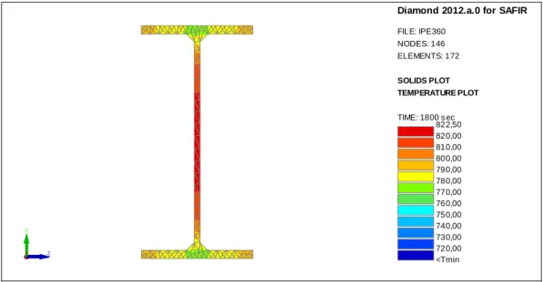
Figure 23: IPE360 heated on 4 sides
Figure 24: 90 mm slab with 5 mm of insulating concrete – discretisation
X
Y
Z
Diamond 2012.a.0 for SAFIR
FILE: IPE360 NODES: 146 ELEMENTS: 172 SOLIDS PLOT TEMPERATURE PLOT TIME: 1800 s ec 822,50 820,00 810,00 800,00 790,00 780,00 770,00 760,00 750,00 740,00 730,00 720,00 <Tmin X Y Z
Diamond 2012.a.0 for SAFIR
FILE: Cof60_90_05 NODES: 50 ELEMENTS: 24 SOLIDS PLOT CONTOUR PLOT SILCONC_EN SILCONC_EN
Figure 25: 90 mm concrete slab with 5 mm insulating concrete – isotherms
2.2 Mechanical simulations
2.2.1 The model
Slab panels are modelled by a combination of 3D Bernoulli beam finite elements and shell finite elements.
Beam elements are used to represent the unprotected steel beams located within the slab panel. Shell finite elements are used to model the concrete slab located on the perimeter beams and on
the unprotected perimeter beams.
The beam elements share their end nodes with the nodes of the shells located above the beams which ensures a full composite action between the beams and the slab.
The level arm between the steel beam and the concrete shell is dully taken into account because the node line of the beam (where the displacements are calculated and the forces are transmitted from element to element) is located at mid-level of the structural part of the concrete slab. Boundary conditions:
The perimeter beams are not modelled explicitly. A perfect vertical support is supposed on the perimeter of the slab panel, in accordance with the hypothesis of the FRACOF method.
No horizontal restrain is provided on the perimeter of the slab panel, in accordance with the hypothesis of the FRACOF method. Only the rigid body movements are prevented to ensure convergence of the model.
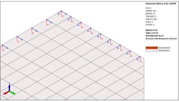
When possible, vertical planes of symmetry are considered and only ½ or ¼ of the slab is modelled. Figure 26 shows a general overview of a slab panel where only ¼ is modelled.
X
Y
Z
Diamond 2012.a.0 for SAFIR
FILE: Cof60_90_05 NODES: 50 ELEMENTS: 24 SOLIDS PLOT CONTOUR PLOT TEMPERATURE PLOT TIME: 1800 s ec >Tmax 800,00 700,00 600,00 500,00 400,00 300,00 200,00 100,00 46,30
Figure 26: 9 x 9 slab panel with 2 steel beams - 1/4 modelled
Figure 27 shows the boundary conditions on the perimeter of the slab panel: the vertical displacement (in red) and one rotation (in blue) are restrained.
Figure 27: Boundary conditions in the corner of the slab panel
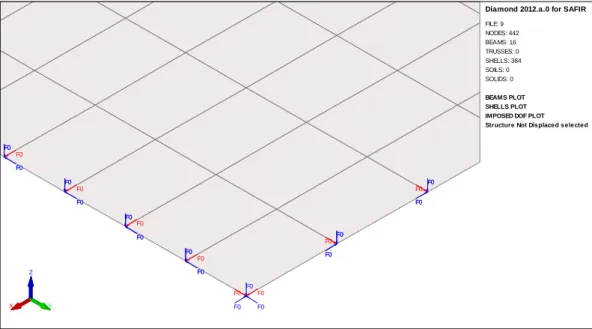
Figure 28 shows the boundary conditions on axes of symmetry of the model: the horizontal displacement perpendicular to the plane of symmetry (in red) and two rotations in the plane of symmetry (in blue) are restrained.
F0 F0 F0 F0 F0 F0 F0 F0 F0 F0 F0 F0 F0 F0F0 F0 F0 F0 F0 F0 F0 F0 F0 F0F0 F0 F0 F0 F0 F0 F0 F0 F0 F0 F0 F0 F0 F0 F0 F0 F0 F0 F0 F0 F0 F0 F0 F0 F0 F0 F0 F0 F0 F0F0 F0 F0 F0 F0 F0 F0 F0 F0 F0F0 F0 F0 F0 F0 F0 F0 F0 F0 F0 F0 F0F0 F0 F0 F0 F0 F0 F0 F0 F0 F0 F0 F0 F0 F0 F0 F0 F0 F0 F0 F0 F0 F0 F0 F0 F0 F0 F0 F0 F0 F0 F0 F0 F0 F0 F0 F0 F0 F0 F0 F0 F0 F0F0 F0 F0 F0 F0 F0 F0 F0 F0 F0F0 F0 F0 F0 F0 F0F0 F0 F0 F0F0 F0 F0 F0 F0 F0 F0 F0 F0 F0 F0 F0 F0 F0 F0 F0 F0 F0 F0 F0 F0 F0 F0 F0 F0 F0 F0 F0 F0F0 F0 F0 F0 F0 F0 F0 F0 F0 F0 F0 F0 F0 F0 F0 F0 F0 F0 F0 F0 F0 F0 F0 F0 F0 F0 F0 F0 F0 F0 F0F0 F0 F0 F0 F0 F0 F0 F0 F0 F0 F0 F0 F0 F0 F0 F0 F0 F0 F0 F0 F0 F0 F0 F0 F0 F0 F0 F0 F0 F0F0 F0 F0 F0 F0 F0 F0 F0 F0 F0 F0 F0F0 F0 F0 F0 F0 F0 F0 F0 F0 F0 F0 F0 F0 F0 F0 F0 F0 F0F0 F0 F0 F0 F0 F0 F0 F0 F0 F0 F0 F0 F0 F0 F0 F0 F0 F0 F0 F0 F0 F0 F0 F0 F0 F0 F0 F0 F0 F0F0 F0 F0 F0 F0 F0 F0 F0 F0 F0 F0 F0 F0 F0 F0 F0 F0 F0 F0 F0 F0 F0 F0 F0 F0 F0 F0 F0 F0 F0 F0 F0 F0F0 F0 F0 F0 F0 F0 F0 F0 F0 F0 F0 F0 F0 F0 F0 F0 F0 F0F0 F0 F0 F0 F0 F0 F0 F0 F0 F0 F0 F0F0 F0 F0 F0 F0 F0 F0 F0 F0 F0 F0 F0 F0 F0 F0 F0 F0 F0 F0 F0 F0 F0 F0 F0 F0 F0 F0 F0 F0 F0F0 F0 F0 F0 F0 F0 F0 F0 F0 F0 F0 F0 F0 F0 F0 F0 F0F0 F0 F0 X Y Z
Diamond 2012.a.0 for SAFIR
FILE: 9 NODES: 442 BEAMS: 16 TRUSSES: 0 SHELLS: 384 SOILS: 0 SOLIDS: 0 NODES PLOT BEAMS PLOT SHELLS PLOT IMPOSED DOF PLOT Structure Not Displaced selected
Beam Element Shell Element F0 F0 F0 F0 F0 F0 F0 F0 F0 F0 F0 F0 F0 F0 F0 F0 F0 F0 F0 F0 F0 F0 F0 F0 F0 F0 F0 F0 F0 F0 F0 F0 F0 F0 F0 F0 F0 F0 F0 F0 F0 F0 F0 F0 F0 F0 F0 F0 F0 F0 F0 X Y Z
Diamond 2012.a.0 for SAFIR
FILE: 9 NODES: 442 BEAMS: 16 TRUSSES: 0 SHELLS: 384 SOILS: 0 SOLIDS: 0 BEAMS PLOT SHELLS PLOT IMPOSED DOF PLOT Structure Not Displaced selected
Beam Element Shell Element
Figure 28: boundary conditions in the center of the slab panel
Compressive strength of concrete is 30 MPa with tensile strength nominally equal to 0 (a value of 0,3 MPa has been used in the models in order to speed up convergence during initial loading). A concrete model that takes transient creep into account explicitly has been considered (Gernay et al, 2013). All models follow Eurocodes recommendations. The composite slab is made of a COFRA+60 trapezoidal sheets. A concrete layer of 90 mm is added on the steel sheets and the ribs are modelled by a 5 mm layer of non-structural concrete. Two layers of reinforcing bars are located at mid-level of the concrete layer (i.e. 45 mm from the top surface) with equal section.
A uniformly distributed load of 6,575 kN/m² was applied corresponding to the dead weight of the composite slab (11,3 cm x 25 kN/m³), plus a permanent load of 1,25 kN/m² + a service load of 0,5 x 5 kN/m² (0,5 x 2,5 kN/m² for the 9 m x 9 m slab panel, see section 2. 2.4).
Each case was modelled by SAFIR and then calculated by MACS+. In MACS+, full composite action between the steel beams and the composite slab has been considered as in SAFIR.
The quantity of reinforcing bar was varied as a parameter.
2.2.2 Mesh sensitivity
A mesh sensitivity analysis has been performed. It is known that, in elastic problems, the results of displacement type finite elements tend toward the numerical true solution when the size of the elements tends toward 0. A balance has nevertheless to be found between a reasonable precision to be obtained and reasonable computation times.
In order to gain insight into the sensitivity of the size of the elements, a 6 m x 9 m slab panel with 1 IPE 400 has been analyzed. ½ of the panel has been modelled owing to symmetry reasons. The slab contains 200 mm²/m of steel in each direction and the total load is 6,58kN/m². The mesh size has
F0 F0 F0 F0 F0 F0 F0 F0 F0 F0 F0 F0 F0 F0 F0 F0 F0 F0 F0 F0 F0 F0 F0 F0 F0 F0 F0 F0 F0 F0 F0 F0 F0 F0 F0 F0 F0 F0 F0 F0 F0 X Y Z
Diamond 2012.a.0 for SAFIR
FILE: 9 NODES: 442 BEAMS: 16 TRUSSES: 0 SHELLS: 384 SOILS: 0 SOLIDS: 0 BEAMS PLOT SHELLS PLOT IMPOSED DOF PLOT Structure Not Displaced selected
been reduced progressively from 300 cm to 20 cm.Table 1 shows the meshes for elements of 300, 100, 50 and 20 cm.
Table 1: four different meshes
The most important results are reported in Table 2. For this slab panel, the software MACS+ gives a fire resistance time of 40 minutes.
Table 2: results of the mesh sensitivity
Size of the elements
Number of elements
End of Run (L+l)/30 CPU time
for 20 minutes of simulation
mm - minutes minutes seconds
300 4 145 76 58 150 12 136 74 209 100 30 99 67 468 75 48 88 61 828 60 80 91 60 1308 50 108 95 60 2016 38 192 58 55 2949 20 660 44 52 9721
The results are depicted in Figure 29.
It shows a bigger mesh sensitivity when the time of last convergence is considered (EoR) than when a displacement criteria is considered. This shows that, when displacements are excessive, the results of the numerical simulation become less and less reliable. This is because, for excessively large
displacements, the basic hypotheses of numerical simulation (small strains, limited rotations…) are more and more violated. Although the simulation produces some results and numbers, these become more and more meaningless.
The time when the displacement criteria (l+L)/30 is met, on the other hand, is much less sensitive to the refinement of the model. It is amazing that, even with only 4 or 12 elements used to model the structure, a rough estimate can be found with an approximation of only 25%. When the mesh varies from 50 to 75 cm, the result varies by only 1 minute. For smaller meshes, distortion of the slab close to the corners has to be accommodated by one single element in which it is concentrated and slightly earlier failure may occur.
The time needed for a simulation of a certain duration of fire is proportional to the number of finite elements.
Figure 29: results of the mesh sensitivity analysis
As a result of this analysis, it is decided not to use shell finite element with a dimension higher than 750 mm. The aspect ratio r of the shell elements must not be too high, certainly not bigger than 2.
2.2.3 7,5 m x 15 m
The first slab panel presented here is a 7,5 m x 15 m slab panel with 2 unprotected IPE 600 in S235 parallel to the long edges, see Figure 30.
The chosen configuration fits nominally with the one described in Fig. 7.42, 6th solution, and Table 7.5 of the ECCS publication N°132.
0
30
60
90
120
150
0
50
100
150
200
250
300
EoR
(L+l)/30
Figure 30: 7,5 x 15 m² (1/4 modelled)
1/4 of the slab panel was modelled owing to symmetry. The beam was modelled by 24 beam finite elements of 312,5 mm and 384 shell finite elements of 227 mm x 312,5 mm (aspect ratio : r =
1,38).
Figure 31, for example, shows the evolution of the vertical displacement in the center of the slab calculated by SAFIR for a reinforcement of 473 mm²/m in each direction as recommended by Table 7.4 of the ECCS publication. The displacement calculated by MACS+ is also given in this Figure. It can be observed that, except during the first 15 minutes of the fire, the displacement calculated by MACS+ is lower than the one calculated by SAFIR. It has to be kept in mind that, in MACS+, the displacement is only an intermediate parameter used to calculated the enhancement factor; the bigger the displacement, the higher the enhancement factor and, hence, the higher the load bearing capacity at any given time.
X Y
Z
Diamond 2012.a.0 for SAFIR
FILE: 11A433x NODES: 450 BEAMS: 24 TRUSSES: 0 SHELLS: 384 SOILS: 0 SOLIDS: 0 BEAMS PLOT SHELLS PLOT
Structure Not Displaced selected
Beam Element Shell Element
SAFIR runs until 105 minutes, time when the strain in the unprotected steel beam reaches 15%; compared to a result of 110 minutes given by MACS+. The fact that the fire resistance time calculated by MACS+ is in the same order of magnitude as the one calculated by SAFIR is amazing considering that the displacement is underestimated by a factor of approximately 1,75 in MACS+. It seems as if some aspects of the mechanical part of the model in the simple method compensate in a way or another the underestimation of the vertical displacement.
It has yet to be discussed whether the displacement of 87 cm calculated by SAFIR after 105 minutes is acceptable, see Figure 33. The deflection is usually compared to the sum of the length of the short and of the long edge of the slab panel, l+L, considering that both primary and secondary beams that form the edges of the slab panel will deflect. Here the ratio after 105 minutes is (l+L)/26. Yet, if the edges of the slab panel are fixed vertically, which is the hypothesis of the simple method, the deflection that will be experienced in the building by the occupants will be related to the short edge as seen on Figure 32 and the ratio is then l/9 ! At this moment, the horizontal displacement on the support, at mid distance of the long edge, is 118 mm, which means that the slab would most likely have lost vertical support.
Figure 33 shows the deformed structure after 105 minutes in an isometric view.
Figure 33: deformed shape after 105 minutes (isometry)
It is not uncommon to limit the deflection to (l/L)/30, equal here to 750 mm. In European testing standards, this deflection is calculated with respect to the position of the structure loaded before the fire (32 mm in Figure 31). In this report, we evaluated the deflection criteria with respect to the initial configuration, i.e. before loading. This is because the deflection calculated by SAFIR is obtained from a model in which the corrugated steel profiles are not present. Whereas this is in line with the hypotheses of the simple method and quite acceptable for the fire situation, this leads to an overestimation of the deflection at room temperature. It was decided here that this value of the deflection after loading can be neglected because, even if it is unknown, we know that it is smaller than the one calculated by SAFIR and hence quite negligible compared to (l+L)/30: here we know that the neglected deflection is less than 32/750 = 4%. The limit of 750 mm (corresponding to a ratio of l/10) is observed after 72 minutes in SAFIR. The horizontal displacement on the support at that time is 85 mm.
In all results obtained by SAFIR, we will mention in this report the time when the (l+L)/30 criteria has been met as well as the time at the end of the calculation with, if it can be determined, the reason that lead to an impossibility for SAFIR to calculate further.
Table 3 gives the results for different values of the rebar quantity, from 142 to 503 mm²/m. In France, it is requested that the stress-related strain in the rebars does not exceed 5%. This value has been obtained in these simulations only for the two lowest reinforcement quantities, 142 and 200 mm²/m. In both cases, the end of run occurred within less than one minute after reaching 5% in the reinforcement. This means that this criteria, if it is applied, does not change the results of the simulations significantly.
It has been verified, for a reinforcement of 400 mm²/m, that the final resistance time is not significantly modified if steel in the beams is allowed to have an infinite plastic behavior (no descending branch). Compared to the steel of the EN 1993-1-2 where the plastic plateau is limited to 15%, the fire resistance time is only modified by 7 seconds. The displacement at the last converged step is somehow increased, from 1,012 meter to 1,074 meter. This exercise has been done to verify that the failure
times are not excessively influenced by the “numerical” problems that arise in the steel beam whereas, in reality, the slab could continue carrying the load for a longer time if the beam would just not be present. Clearly, this is not the case.
Table 3: results for the 7,5 m x 15 m slab panel
As MACS+ SAFIR EoR SAFIR (L+l)/30
mm²/m min. Min. Reason
142 22 21 No convergence 23 200 24 32 SdB in shell 31 250 25 39 No convergence 38 300 28 52 SdB in beams 48 350 34 55 375 40 58 400 60 91 SdB in beams 62 433 90 105 SdB in beams 66 473 111 105 SdB in beams 72 503 119 115 SdB in beams 76
Note: SdB means “Steel in Descending Branch” (ɛ > 15%), EoR means “End of Run”, which is the time of last converged solution obtained by SAFIR.
Figure 34 shows the results in a graphic form. It can be observed that MACS+ yields safe results compared to the values provided by the numerical calculation if the end of run is considered. If a displacement limit is considered in the numerical calculations, MACS+ is still on the safe side for low reinforcement quantities (corresponding to R30 and R60) whereas it is not on the safe side for higher reinforcement quantities (corresponding to R90 and R120).
It has to be noted that, in order to consider the same hypotheses as MACS+, the numerical simulations have been performed with vertically fixed edge perimeters. If the deformation of the perimeter beams would be considered in the numerical simulations:
1) the numerical model would predict higher displacements than the displacements presented here; 2) there would be additional stresses in the concrete due to composite action with the perimeter
Figure 34: results for the 7,5 x 15 slab panel
2.2.4 9 m x 9 m
A 9 m x 9 m slab panel was then modelled, with 2 IPE 360 unprotected beams. The characteristic value of the life load considered here is 2,5 kN/m². All other conditions are similar to the slab modelled in previous section. This corresponds to case N° 3 of Figure 7.42 in the ECCS document. The results are presented in Figure 36. ¼ of the slab was modelled owing to symmetry reasons. ¼ of a beam was modelled with 16 beam elements of 188 mm and 384 shell elements of 281 mm x 188 mm (aspect ratio r = 1,49) see Figure 35.
Figure 35: 9 m x 9 m model deformed
The results are presented on Figure 36 and in Table 4. 0 30 60 90 120 100 150 200 250 300 350 400 450 500 550 600 Tim e [m in] As [mm²/m] SAFIR EoR SAFIR (L+l)/30 MACS+
The curve labelled “MACS+” represents the results of the Bailey-Moore method applied in the MACS+ software.
The curve labelled “SAFIR (EoR)” presents the values obtained at the End of Run of the numerical calculation (last converged point).
The curve labelled “SAFIR (l+L)/30” represents the time when the displacement criteria (l+L)/30 was met. The points of this curve located above the “EoR” curve have been obtained by linear extrapolation of the displacement curve beyond the last converged time.
Figure 36: results for the 9 m x 9 m slab panel
Table 4: results for the 9 x 9 slab panel
As MACS+ SAFIR EoR
SAFIR (L+l)/30
mm²/m min. min. Reason min.
100 22 18 Strains in bars 19 166 65 23 SdB in the corner 33 177 88 32 SdB in the corner 34 193 111 38 SdB in the corner 38 252 147 69 SdB in the corner 72 312 180 108 SdB in beams 102 393 143 SdB in the corner 125
For this configuration, the end of convergence obtained by SAFIR was systematically obtained when the maximum deflection in the slab was close to (L+l)/30. In one single case (As = 100 mm²/m), a converged time step was obtained with the strain in a bar larger than 5%. The last converged step
0 30 60 90 120 150 180 0 50 100 150 200 250 300 350 400 450 500 Tim e [m in] As [mm²/m] MACS+ SAFIR EoR SAFIR (L+l)/30
followed only 12 seconds later. This means that failure was imminent in the numerical modelling when a value of 5% was reached for the elongation in the bars. This limitation does not change significantly the fire resistance time when it is applied.
The times calculated numerically, either for the deformation criteria or for the end of convergence, are smaller than the fire resistance times yielded by MACS+.
The difference is very small for AS ≈ 100 mm²/m, but the fire resistance time is not significant for this steel quantity because it is shorter than 30 minutes.
The difference is huge for higher steel quantities. For example, 110 mm²/m are sufficient to yield R30 according to MASC+ whereas 177 mm²/m are required according to SAFIR (+ 61%). If 200 mm²/m are used, MASC+ gives a fire resistance time of nearly 120 minutes whereas SAFIR gives only 45 minutes. With 300 mm²/m, MACS+ gives nearly 180 min when SAFIR gives only some 100 minutes.
The evolution of the displacement in the center of the slab as calculated by SAFIR and estimated by MACS+ is shown on Figure 37 for As = 193 mm²/m.
It has been mentioned that, for the rectangular slab of Section 2.2.3, the displacement was underestimated by MACS+ but the ultimate load bearing capacity was on the safe side compared to numerical modelling. For the square slab of this section, the displacement at failure is rather well estimated by MACS+ but the ultimate load bearing capacity is now very much on the unsafe side. This seems to confirm that the mechanical model of MACS+ based on the displacement could be unsafe and, when the displacement is underestimated, both errors tend to compensate each other.
Figure 37: vertical displacement in the center of the 9 x 9 m² slab -0,7 -0,6 -0,5 -0,4 -0,3 -0,2 -0,1 0 0 1000 2000 3000 4000 5000 6000 7000 SAFIR MACS+
2.2.5 6 m x 6 m
A slab panel of 6 m x 6 m with 1 unprotected IPE 270 in S235 has been analyzed. This configuration fits nominally with the one described in Fig. 7.42, 1rst solution, and Table 7.5 of the ECCS publication N°132. ½ of the slab panel was modelled owing to symmetry. ½ of the beam was modelled by 10 beam finite elements of 300 mm and 1/2 slab by 200 shell finite elements of 307 mm x 302 mm (aspect ratio: r = 1,02). Figure 38 shows the model deformed at the end of the run with a mesh of 125 mm²/m in each direction. The deflection at the center of the slab is equal to 479 mm. This deflection corresponds to l/13.
Figure 38: 6 m x 6 m model deformed
The results are given in Figure 39 and in the Table thereafter. The value of 5% for the mechanical strain in the reinforcing bars was not obtained in any of the simulations. The deflection (L+l)/30 corresponds to a deflection of 400 mm. This deflection corresponds to l/15.
2.2.6 6 m x 12 m
A slab panel of 6 m x 12 m with 1 unprotected IPE 600 in S235 parallel to the long edges has been analyzed. This configuration fits nominally with the one described in Fig. 7.42, 4th solution, and Table 7.5 of the ECCS publication N°132. The entire slab panel was modelled here. The beam was modelled by 24 beam finite elements of 500 mm and the slab by 384 shell finite elements of 500 mm x 375 mm (aspect ratio: r = 1,33), see Figure 40.
.
Figure 40: 6 m x 12 m model
The results are given in Figure 41 and in the Table thereafter. The value of 5% for the mechanical strain in the reinforcing bars was not obtained in any of the simulations. The deflection (L+l)/30 corresponds to a deflection of 600 mm. This deflection corresponds to l/10.
As MACS+ SAFIR (L+l)/30
mm²/m min. min. Reason min.
100 23 47 SdB in the corner shell
112 25
125 30 56 SdB in beams 39
138 42
150 83 64 Error in concrete 56
175 118 82 No convergence 79
200 134 118 SdB in the corner shell 108 SAFIR EoR
Figure 41: results for the 6 x 12 slab panel
As MACS+ SAFIR EoR
SAFIR (L+l)/30
mm²/m min. min. Reason min.
200 24 47 No convergence 38 300 40 100 SdB in beams 64 350 97 114 SdB in beams 75 400 121 117 SdB in beams 89 500 152 148 SdB in beams 107
2.2.7 9 m x 12 m
A slab panel of 9 m x 12 m with 2 unprotected IPE 600 in S235 parallel to the long edges has been analyzed. This configuration fits nominally with the one described in Fig. 7.42, 5th solution, and Table 7.5 of the ECCS publication N°132. ½ of the slab panel was modelled owing to symmetry. Each ½ beam was modelled by 12 beam finite elements of 500 mm and 1/2 slab by 216 shell finite elements of 500 mm x 500 mm (aspect ratio: 1,00). Figure 42 shows the model deformed when the deflection at the center of the slab is equal to (L+l)/30 = 700 mm. This deflection corresponds to l/13.
Figure 42: 9 m x 12 m model deformed
The results are given in Figure 43 and in the Table thereafter. The value of 5% for the mechanical strain in the reinforcing bars was not obtained in any of the simulations. For some simulations, the time corresponding to (L+l)/30 is slightly longer than the time of the End of run. For these cases, the time corresponding to (L+l)/30 has been extrapolated beyond the End of Run in the time-displacement curve.
Figure 43: results for the 9 m x 12 m slab panel
0 30 60 90 120 150 180 100 150 200 250 300 350 400 450 500 550 600 Tim e [m in] As [mm²/m] SAFIR EoR SAFIR (L+l)/30 MACS+
Results for the 9 m x 12 m slab panel
As MACS+ SAFIR EoR
SAFIR (L+l)/30
mm²/m min. min. Reason min.
200 25 24 No convergence 25 250 30 31 No convergence 32 275 40 34 No convergence 35 300 85 40 SdB in the corner 41 400 137 68 No convergence 65 500 170 86 SdB in beams 91
2.2.8 9 m x 15 m
A slab panel of 9 m x 15 m with 2 unprotected IPE 500 in S235 parallel to the long edges has been analyzed, see Figure 44. This configuration fits nominally with the one described in Fig. 7.42, 7th solution, and Table 7.5 of the ECCS publication N°132. The entire slab panel was modelled here. Each beam was modelled by 20 beam finite elements of 750 mm and the slab by 300 shell finite elements of 600 mm x 750 mm (aspect ratio : r = 1,25).
Figure 44: 9 m x 15 m model
The results are given in Figure 45 and in the Table thereafter. The value of 5% for the mechanical strain in the reinforcing bars was not obtained in any of the simulations. The deflection (L+l)/30 corresponds to a deflection of 800 mm. This deflection corresponds to l/11.
Figure 45: results for the 9 x 15 slab panel
Results for the 9 m x 15 m slab panel
2.2.9 3 sides heating versus 4 sides heating
All simulations performed in the ECCS document as well as in this document are performed with a composite slab made of a COFRA+60 steel sheet. Because this sheet covers less than 90% of the upper flange of the steel section, the steel section is heated on 4 sides.
Yet, if the steel sheet is a reentrant profile (e.g. Hollerith type), more than 90% of the upper flange is covered by the composite slab and the steel beams have to be modelled as exposed to three sides only. This will induce a thermal gradient in the steel beam that is likely to increase the vertical displacements in the slab panel. We investigated whether this could have a detrimental effect on the behavior of the slab panel.
The temperatures in the IPE360 beam have been calculated on the hypothesis that it is heated on 4 sides first, see Figure 46, then on 3 sides, see Figure 47.
0 30 60 90 120 150 180 100 150 200 250 300 350 400 450 500 550 600 650 700 Ti me [min ] As [mm²/m] SAFIR EoR SAFIR (L+l)/30 MACS+ As MACS+ SAFIR (L+l)/30
mm²/m min. min. Reason min.
200 21 23 No convergence 23 300 24 35 No convergence 35 400 80 51 No convergence 47 500 127 69 SdB in beams 62 600 153 99 SdB in beams 76 SAFIR EoR
Figure 46: temperatures after 30 minutes (4 sides heated)
Figure 47: temperatures after 30 minutes (3 sides heated)
The 9 m x 9 m slab panel with reinforcement of 193 mm²/m has been calculated on the base of these two hypotheses. The evolution of the displacement in both hypotheses is presented in Figure 48.
The displacement is indeed slightly bigger when the beams are heated on 3 sides but not to an extent that would affect significantly the time when a displacement criterion would be met. The time of failure (last converged point) is higher with 4 sides exposure (1 min 30 sec), with the displacement being the same when the vertical asymptote begins.
X
Y
Z
Diamond 2012.a.0 for SAFIR
FILE: IPE360 NODES: 146 ELEMENTS: 172 SOLIDS PLOT TEMPERATURE PLOT TIME: 1800 s ec 822,50 820,00 810,00 800,00 790,00 780,00 770,00 760,00 750,00 740,00 730,00 720,00 <Tmin X Y Z
Diamond 2012.a.0 for SAFIR
FILE: IPE360_3faces NODES: 146 ELEMENTS: 172 SOLIDS PLOT TEMPERATURE PLOT TIME: 1800 s ec 822,10 820,00 810,00 800,00 790,00 780,00 770,00 760,00 750,00 740,00 730,00 720,00 <Tmin