ANOMALOUS PERTURBATIVE TRANSPORT IN TOKAMAKS DUE TO DRIFT-WAVE TURBULENCE

Anomalous perturbative transport in tokamaks due to driftwave turbulence

Anne A. Thoul, P. L. Similon, and R. N. Sudan

Citation: Phys. Plasmas 1, 579 (1994); doi: 10.1063/1.870803 View online: http://dx.doi.org/10.1063/1.870803

View Table of Contents: http://pop.aip.org/resource/1/PHPAEN/v1/i3 Published by the American Institute of Physics.

Additional information on Phys. Plasmas

Journal Homepage: http://pop.aip.org/

Journal Information: http://pop.aip.org/about/about_the_journal Top downloads: http://pop.aip.org/features/most_downloaded Information for Authors: http://pop.aip.org/authors

Anomalous perturbative transport in tokamaks due to drift-wave

turbulence

Anne A. Thoul

Institute for Advanced Study, Princeton, New Jersey 08540 P. L. Similon

Department of Applied Physics, Yale University, New Haven, Connecticut 06520 R. N. Sudan

Laboratory for Plasma Studies, Cornell University, Ithaca, New York 14853 (Received 9 April 1993; accepted 29 October 1993)

A new method for calculating the anomalous transport in tokamak plasmas is presented. The renormalized nonlinear plasma response function is derived using the direct-interaction approximation (DIA). A complete calculation for the case of electrostatic drift-wave turbulence is presented. Explicit expressions for all coefficients of the anomalous transport matrix relating particle and heat fluxes to density and temperature gradients in the plasma are obtained. The anomalous transport matrix calculated using the DIA does not have the Onsager symmetry. As an example of application, the parameters of the Texas Experimental Tokamak (TEXT) [Nuc!. Technol. Fusion 1, 479 (1981)] are used to evaluate all transport coefficients numerically, as well as the spectrum modulation. The relation between the theoretical results and the experimental data is discussed. Although this paper focuses on electron transport for simplicity, the method can also be used to calculate anomalous transport due to ion instabilities, such as the ion-temperature-gradient instability.

r.

INTRODUCTION

To sustain thermonuclear reactions in a tokamak, the plasma must be confined well enough to overcome heat losses. The confinement of the energy for a long enough time is a major difficulty in magnetic fusion.

It is well known that classical calculations of heat dif-fusion based on kinetic theory (using, for example, the Fokker-Planck or Balescu-Lenard collision operators; see, e.g., Braginskii1 or Hinton2) yield transport coefficients which are in complete disagreement with observations. 80-called "neoclassical" transport theories are still based on classical collisional processes, but take into account the toroidal geometry of a tokamak. 3,4 According to neoclas-sical theories, the electron heat conductivity is smaller than the ion heat conductivity by a factor ~melmi' However, measurements (in Ohmic discharges) indicate that, al-though the ion heat transport appears to be well described by neoclassical results,5-7 the electron heat transport is sometimes as much as two orders of magnitude larger.5

,8 The energy transport is therefore completely dominated by the electrons in those cases. This so-called "anomalous transport" is the subject of this work.

Today, the design of fusion reactors relies heavily on empirical scaling laws deduced from extrapolation of ex-isting experimental data.9-11 Unfortunately, these

extrapo-lations are unreliable, since the parameters of future reac-tors are often very different from those of existing machines. A more fundamental understanding of transport in tokamak plasmas is therefore critical to the design of future generations of reactors. 12 Recent reviews on the present status of experiments and theoretical models can be found in Boozer et aZ., 13 Wootton et al., 14 Burrel et al., IS

Houlberg et al., 16 and Kaye et al.17

It is now widely accepted that the anomalous transport in tokamaks results very likely from the presence of a sat-urated spectrum of fluctuations in the plasma, produced by microscopic turbulence (see, e.g., the reviews by Tang,8 Horton,18 and LiewerI9). For example, in the presence of

fluctuating electric fields, transport of particles across the magnetic flux surfaces can occur through the EX B drift. In the presence of fluctuating magnetic fields, the magnetic flux surfaces are destroyed and electrons can flow outward along the perturbed field lines. Possible sources of turbu-lent fluctuations include drift modes,20-23 dissipative trapped electron (DTE) modes,24 ion-temperature-gradient modes,25,26 electron-temperature-gradient modes,27 and microtearing modes.28

The relatively low frequency (cu;$ 0.5 MHz<!li' the ion Larmor frequency) of small-scale (k1 Pt;$l) density and potential fluctuations observed in some tokamak experiments29_-32 suggests that drift waves and DTE modes may be responsible for the anomalous transport. Drift waves are unstable, low-frequency waves produced in any plasma having spatial inhomogeneities and a magnetic field. They propagate mainly in the direction perpendicular to both the density gradient and the magnetic field, but they have a finite parallel wave number, which allows elec-trons to flow freely along the field lines. Their simplest dispersion relation is of the form cu

=

k • v

* '

where v*=-(cT/eB)boX(Vnolno) is the diamagnetic drift ve-locity (see, e.g., Nicholson33 ). Recently, it has become ev-ident that the ion dynamics can also playa crucial role in the anomalous transport because of the ion temperature gradient ('TIt> instability.25,26 Indeed, it has been observed that the Ohmic confinement time saturates at high density an order of magnitude below the predictions of neoclassical

theory, indicating anomalous ion losses.34 In addition, it

was observed that pellet injection improves the ion energy confinement, while leaving the anomalous electron thermal losses unchanged.35 Far-infrared laser scattering experi-ments on the Texas Experimental Tokamak (TEXT)36 showed that the onset of fluctuations propagating in the ion direction coincides with the saturation of the energy confinement time with density,37 which strongly suggests an association between the anomalous ion losses and the saturation of the energy confinement time.

Many calculations of anomalous transport have been performed3_{!41 in the so-called "quasilinear"}

approxima-tion of weak-turbulence theory (see, e.g., Kadomtsev42 and Sagdeev and Galeev43 ). In these calculations, the level of turbulence is assumed to be low enough so that the non-linearities can be treated perturbatively. To obtain closure, the weak-turbulence expansion must be truncated to some order. The "quasilinear" theory corresponds to truncating this expansion to first order.42,43 The transport can be cal-culated from correlations of fluctuations, obtained from the linearized equations. The important effect considered in quasilinear theory is the wave-particle interaction, but the mode-mode coupling terms are neglected. However, exper-iments suggest that mode-mode coupling effects are, in fact, very important, and that the weak-turbulence condi-tion is usually not satisfied.3o

In a strongly turbulent plasma, the nonlinearities are essential and the perturbative approach of weak-turbulence theory fails. The goal of renormalized plasma turbulence theories is to simplify the nonlinear problem by attempting to describe only the macroscopic statistical averages of the fluctuations. Examples of such renormalization techniques include the "resonance broadening,,44 and "clump,,45 cal-culations, as well as methods based on the direct interac-tion approximainterac-tion. 42.~9 Renormalization prescriptions are generally untested closure assumptions, which should be treated with caution. However, the direct interaction approximation (hereafter DIA) provides an exact descrip-tion of certain stochastic models, such as the random-coupling model 50 and the Langevin equation.SI

Further-more, the DIA method automatically satisfies the self-consistency constraints arising from the strong coupling between electromagnetic fields and particle densities through Maxwell's equations. These constraints are not satisfied in quasilinear calculations.

Since the DIA method is based on the evaluation of averaged infinitesimal response functions, it naturally pro-vides the incremental./luxes resulting from small perturba-tions of the equilibrium profiles, rather than total fluxes accross the magnetic surfaces. 52 It is therefore particularly

well suited to comparisons with the recent gas puffing, pel-let injection, and heat pulse propagation experi-ments.15_•5_{3-56 These experiments are performed either by}

using externally imposed modulated sources or by taking advantage of naturally occurring phenomena such as saw-teeth oscillations. 56-59 In contrast to quasilinear calcula-tions, we will show that the DIA formalism can also be used to study the modulation of the fluctuation spectrum caused by external modulated perturbations. Such

spec-580 Phys. Plasmas, Vol. 1. No.3, March 1994

trum modulation measurements have been performed re-cently in TEXT.

Traditionally, the transport of particles and heat in tokamaks have been studied as two independent problems, with the particle flux related to the density gradient by Fick's law,

r= -

D Vn, and the heat flux expressed in terms of the temperature gradient as q=

-nx

VT. In these simple laws, the diffusion coefficient D was assumed to be independent of the temperature gradient, and the heat con-ductivity X was assumed to be independent of the density gradient. However, recent experimental and theoretical studies have shown that it is incorrect to assume no cou-pling between energy and particle transport.59-61 If the

transport is due to turbulence, the coefficients D and X will

be functions of the plasma parameters. Any theory of tur-bulent transport should therefore produce a full transport matrix, including off-diagonal coefficients, rather than just two coefficients D and X (see Gentle et al. 61 ) .

In this work, we use the DIA technique to calculate the transport matrix ( diagonal and off-diagonal coeffi-cients) corresponding to perturbations in the density and temperature profiles. The theoretical expressions obtained for the transport coefficients are based on a specific set of equations describing the dynamics of the plasma and on the DIA, but do not require any further approximations.

Even though the current interpretation of transport experiments in tokamaks is that the ion dynamics plays a crucial role in the anomalous thermal transport, we con-centrate, for simplicity, on the role played by the electrons, and give the ions a secondary role in this paper. Our method can, in principle, account for the ion dynamics as well by choosing an appropriate form for the ion nonlinear susceptibility (see Sec. II). Here, however, detailed numer-ical estimates are given only for a very simple ion suscep-tibility, which does not necessarily represent the complete physics of anomalous transport in tokamaks. This choice is discussed in more details in Sees. III and IV. In addition, we use the simplest possible model for the electrons them-selves, ignoring the complications coming from the toroi-dal geometry, such as magnetic curvature and shear. With these simplifying assumptions, we are able to present a completely self-consistent, yet tractable calculation of anomalous transport in a strong-turbulence regime.

Our work is presented in two papers. In this paper we consider the transport due to electrostatic drift-wave tur-bulence. In a companion paper,62 we use the method de-veloped here to calculate the transport due to drift-Alfven wave turbulence, i.e., including the effects of magnetic fluc-tuations.

This paper is organized as follows. In Sec. II, we give the basic assumptions and the model equations describing the dynamics of the plasma. We present a method based on the DIA to calculate the transport matrix coefficients. The results are given in a very general form, in terms of the potential fluctuation spectrum. In Sec. III, we give a brief review of fluctuations and transport experiments. As an example of application of our method, we give numerical estimates of the transport coefficients corresponding to the

parameters of the TEXT tokamak. Finally, in Sec. IV, we give a summary of the principal results.

II. ANOMALOUS TRANSPORT FROM DRIFT-WAVE TURBULENCE

In this section, we develop a method to determine the transport coefficients associated with drift-wave turbulence in a tokamak plasma. In Sec. II A, we introduce the fun-damental kinetic equations, which serve as a basis for the theory, and we specify the geometry of the problem. In Sec. II B, we exploit the separation of time scales and length scales in the problem to derive two separate systems of equations: one describing the transport, the other describ-ing the turbulent fluctuations. Finally, in Sec. II C, we derive a statistical solution for these equations using the direct interaction approximation (DIA), and we give ex-plicit expressions for the anomalous fluxes of particles and heat.

A. Basic equations

1. Electron dynamiCS

When considering plasma phenomena of low fre-quency compared to the electron gyrofrefre-quency, such as drift waves, the electron dynamics can be described by the drift-kinetic equation (hereafter DKE). This equation de-scribes the motion of the guiding center of the particles, and is obtained by averaging the Vlasov equation over the rapidly oscillating component of the motion (see, e.g., Kulsrud63 and Landau and Pitaevskii64). It is given by

al

a

-a +Vo[(vE+vD)/]+Vo(vllb/)+-a

t ~

x[(

-~eEIl -~eboVB)f]=C(f),

(1)

where l(x,vlI ,/L,t) is'the electron distribution function,

/L=mevI/2B is the electron magnetic moment, C(f) is the collision operator, and parallel

II

and perpendicular 1 subscripts refer to· the direction of the magnetic field. In this equation, the EXB drift velocity is given by

VE= (el B)EXb, while the magnetic drift velocity

vD=(lI Bfie)(v~ /2)bXV B+(lIfie)vrr (RBXb), where

b is a unit vector parallel to the magnetic field, fie is the electron gyrofrequency, and RB is vector curvature radius of the magnetic field lines.

In this section, we will consider the electrostatic limit (E= - V<,b, where <,b is the electrostatic potential) of the DKE, which is valid when the plasma parameter

(3«m/mi) (see, e.g., Miyamot065). We consider the more

general electromagnetic case [E

= -

V <,b - ( lie) aAJ at] in Paper II. We distinguish between the two different popu-lations of electron in a tokamak: circulating and trapped

(see, e.g., Miyamot065). In this work, for simplicity, we

ignore the magnetic shear66 and curvature in the tokamak, i.e., we consider a uniform magnetic field Bo. As a conse-quence, v D=O and V B=O. The presence of trapped parti-cles is therefore the only VB effect that we consider.

The circulating electrons have 1 vII IVI 1 > (2£) 112,

where £=rIR is the inverse aspect ratio of the tokamak (r Phys. Plasmas, Vol. 1, No.3, March 1994

and R are the minor and major radii of the tokamak). The orbits of circulating electrons have no turning points; hence they "circulate" around the torus. The distribution function r(x,vII

,vr

,t) of circulating electrons obeys the following DKE;

ar

Tt+VEo V r+vlI

The collision operator C_c will be specified below [Eq.

(25)].

The trapped electrons, instead,. have 1 VII IVI 1

< (2£) 112, implying the presence of turning points in their

orbits ("banana orbits;" see, e.g., Miyamot06S). For these

electrons, the DKE can be further simplified by "bounce averaging," i.e., averaging over the rapid oscillatory mo-tion of the guiding center in the toroidal direcmo-tion. The bounce-averaged DKE is valid for frequencies smaller than the bounce frequency, i.e., for W<wbe= [ev/(Rq), where

ve

==

~T oIme is the electron thermal velocity, To is the elec-tron temperature, me is the electron mass, and q is the tokamak safety factor (see, e.g., Gross67). The

bounce-av~raging procedure eliminates all the terms that are odd

in VII from the DKE. The distribution function

.f(XI ,vI ,t) for the trapped electrons therefore satisfies

a.f

t t

ai+VEoV

I

=Ct(r.t). (3)

2. Ion· dynamics

Our work will focus on the electron nonlinearities. For simplicity, the ion dynamics will be treated in the fluid limit. In this limit, the ion density ni can be written quite generally as68,69

(4)

where no is the eqUilibrium ion density (we take Z=l),

and Xi(

1

<,b

12)

is the nonlinear ion susceptibility, which de-pends on the frequency and the power spectrum of the potential fluctuations. The results of this section are given in terms of an unspecified Xi' In Sec. III we will introduce

a specific form for Xi' which will allow us to obtain

nu-merical results.

3. Self-consistency constraint

It is important to maintain the self-consistency of the model, since the electromagnetic fields and particle densi-ties are strongly coupled through Maxwell's equations. Theories that are not self-consistent, such as those based on the quasilinear approximation, usually violate the impor-tant property of ambipolarity of the particle fluxes.4o

Here the system of equations (2)-(4) describing the particle and field dynamics is closed by the addition of the quasineutrality relation, valid for scales larger than AD (the Debye length),

(5) Thoul, Similon, and Sudan 581

where ne(x,t) =

I

fe dv=

I

ere

+

f)dv is the total electron density.

4. Geometry

Since we assume that Bo is uniform and that the tur-bulent length scale is smaller than the macroscopic scales on which density and temperature vary (cf. Sec. II B), the problem can be studied locally. We can therefore use a local Cartesian geometry, in which x;;;'O represents the ra-dial coordinate, y represents the poloidal coordinate, and z is the coordinate along the field line. The origin is at the center of the minor radial section of the tokamak. The magnetic surfaces are therefore planes with x=const. Note that the plasma density and temperature are constant on magnetic surfaces (see, e.g., Gross67).

B. Separation of scales

1. Motivation

For our study of anomalous transport, the basic set of equations [(2)-(5)] can be rewritten as two separate sys-tems of equations: one describing the turbulence, the other describing the transport. This separation can be done be-cause turbulence and transport correspond to widely dif-ferent time scales and length scales. The two systems of equations remain coupled through their nonlinear terms.

For drift-wave turbulence the typical frequencies and wave numbers are cu-cu*, kl -p;l, and kll _(qR)-I, where cu*=-(cToIeB)koboX(Vnolno) is the electron diamagnetic frequency, Ps is the ion gyroradius at the elec-tron temperature, and qR is the connection length (I.e., the length of the helical trajectory of a circulating particle; see, e.g., Gross67). In contrast, the transport occurs at the very

low frequency cuo, and very small wave number

ko

of the external perturbations. For example, the typical frequency for modulated gas puff experiments in the Texas Experi-mental Tokamak (TEXT) is cu_o:S240 rad/s<cu*-106 radls (cf. Table I). The poloidal and parallel wave num-bers for the transport both vanish because the fluxes are averaged over the magnetic surfaces (perpendicular to the x axis). The radial wave number kox-L;;I<p;l, where Ln==

I

nofVno

I

is the (macroscopic) density gradient length scale. For example, in TEXT, kox=O.04 cm-I and p;I=8 cm-I _{(cf. Table I).}

2. Transportequafions

In the following calculations, we will use an overcaret for quantities that vary on the transport scales, and an overtiide for turbulent quantities. Subscripts 0 will be used for the equilibrium values of the parameters.

In this work, we develop a method to calculate the anomalous fluxes resulting from small external perturba-tions. We study the modulation due to these perturbations on the transport scales. Therefore, we add external, infin-itesimal, velocity-dependent source terms

gc,

g.',

and

g.i

to Eqs. (2), (3), and (4) respectively. As described in Sec.

n

B, these sources have frequencies cuo<cu* and wave num-bers kox

<

p; I. The electron distribution functions

r·

t are

582 Phys. Plasmas, Vol. 1, No.3, March 1994

then the sum of an equilibrium part fo, a fluctuating part

]c,t,

and the response to the modulation

r,t:

(6) where the equilibrium distribution function fo is a local Maxwellian,

no(x)

(T

o

(X»)-3/2

(-meD

2) fo{x,v2) (21T)3/2

----m;-

exp 2T

o(x) , (7) no and To being the local electron density and temperature. We assume70 tPo=O.

The egua!ions describing the (infinitesimal) response functions ft,

r,

Iii. and tP to the external perturbations are obtained by taking the low-frequency and long-wavelength limit of Eqs. (2)-(5), and averaging over the magnetic flux surfaces (Le .• kll 0=0). This gives

(8)

(9)

(10)

(11 )

where the angular brackets denotes an ensemble average over the turbulence. Equations (8) and (9) can also be written in terms of the incremental anomalous fluxes rc,t

==

(v;r·t) as 71

aJctt

A A A

Tt+

V· rc,t= (Ce,t>

+SC,t.

(12)

These phase-space fluxes fe·t are velocity dependent. How-ever, since the collision frequency Vei>wO, the distributions

jc

and

jt

are nearly Maxwellian on transport scales. Therefore we can use the corresponding moment equations to calculate the fluxes of particles and energy. These are obtained by integrating (12) over velocity. We obtain

(13)

where the particle flux density

(14) and

(15)

3 ~ h

where u= ('i)nT is the energy density and

Q==

To

I

(fe+rt)(v2_{/2v;)dv is the total energy flux density.}

Us-ing the continuity equation (13), the energy equation ( 15) can be rewritten as an evolution equation for the temperature,

where the net energy flux

q

is obtained by substracting the energy convected by the particles from the total energy flux Q,

2 3 2

A 3 A

J

A A V - Ve

q=Q-2

Torn

=

To (re+rt) 2v; dv. (17)

Note that we have omitted the terms representing the clas-sical and neoclasclas-sical fluxes (Le., those corresponding to the collision terms

(Get»

in Eqs. (15) and (16).

To evaluate

r

nand

q,

we consider perturbations of the equilibrium density and temperature profiles. The Max-wellian distribution depends on the temperature and den-sity as _{100:. no Tr;3/2 exp( -mif/2To)' Therefore, if we} perturb the density profile, 10 is perturbed according to

al

o

no

no~=/o-,

ano no

and the corresponding sources are

'" "'t •

no

SC=s =

-lwofo - , no " I

J"

5

1 = - . -

se

dv=no·

-lwO (18)

If we perturb the temperature profile, 10 is perturbed

ac-cording to

2 2. A

A alo v -3V;; To

To aT _o =/0 2V2 _e T' ₀

and the sources are

(19)

A 1 J~ A

5

1_{= - . -}

se

_dv=O.

-lwO

Note that in both cases we insist on injecting the same number of ions and electrons in order to preserve the quasineutrality of the plasma.

3, Turbulence

The anomalous fluxes

r

e•t depend on the turbulent

spectrum of fluctuations. These fluctuations are described by the following set of nonlinear equations:

a-

-

-at

Jf+VE' V lo-C

_t=

-VEo V

It,

nl

e¢

-=-Xj,

no To

Phys. Plasmas. Vol. 1, No.3, March 1994

(21 )

(22)

(23)

obtained from Eqs. (2)-(5) by using the expansion (6). We have neglected the nonlinear term

- (e/me)VII ~

al/avil

,sincethis term does not contribute directly to the spatial fluxes.

Vie now specify the form of the collision operators Ce

and Ct. On the time scale of drift-wave turbulence, the

circulating electrons are collisionless, since

w*>vej.

The trapped electrons, however, have an effective collision fre-quency Veff-w*

<

Wb' This "detrapping" frequency is

ve-locity dependent, and is given b}' V_elf=V*(V/v)3, where

v*=v

e

/€.

Some authors have used very simple collision

operators, given by ~

C

t

=

-vefflt,

(24) However, these collision operators do not conserve the number of particles, since electrons detrapped by a colli-sion do not reappear as circulating electrons. Therefore, the use of Eqs.·(24) could introduce errors in the calcula-tion of the transport. A better choice would be to adopt an energy-dependent linearized BGK operator (Bhatnagar, Gross, and Krook72) of the type

(25)

Cc=_(/o)

r

Ctdv,

nOe

J

t

where, ne=~+~ is the total fluctuating electron density, and nOe=

f

clo dv is the equilibrium number density of cir-culating electrons. This collision operator not only con-serves the total number of particles, but also vanishes when

I

is a perturbed Maxwellian. Unfortunately, it couples the two electron equations [(20) and (21)] through their non-linear terms. Although we could, in principle, solve the problem with this collision operator, it complicates the al-gebra substantially. For the sake of simplicity and clarity, we will replace

ne

and_Te in Eq. (25) by their linear ap-proximations

nf

and

Tf,

given by

(26) and -L 2 2. -Te _~

J

-L V - 3ve

=:

e<fJ L T _o -3 _no

I

2 _v" 2 dV-3 T Xr,· 0 (27)

where

I

L

=

(ft+ ft)

L is determined from the linearized

form of Eqs. (20)-(23). Explicit expressions for

xf

(the electron susceptibility) and Xf are derived in Appendix B.

c.

Statistical solution of the model equations

1. The direct interaction approximation

In well-developed turbulence, perturbed quantities can be treated as statistical variables. The equations for the moments of these statistical variables form an infinite set of

differential equations. The direct interaction approxima-tion (hereafter DIA) method provides an approximate way of closing this infinite set of coupled equations into a definite set, containing only moments below some finite order. It presents many advantages over alternative theo-ries of turbulence. In particular, it conserves energy and the positivity of the energy spectrum, two important fea-tures that are not present in simpler theories such as those based on quasinormal approximations.46

In principle, the DIA method allows the determination of both the response functions and the turbulent spectrum at saturation. Here, however, we will use the method to determine the response functions in terms of the saturation spectrum, which we assume to be known experimentally

(see Sec. III).

The DIA method is based on the evaluation of average infinitesimal response functions that naturally provide the

incremental fluxes reSUlting from small perturbations of

the eqUilibrium profiles, rather than total fluxes accross the magnetic surfaces. 52 This is particularly well suited to com-parisons with the recent perturbative transport experiments. 15,61 Indeed, although anomalous transport has been studied traditionally in terms of total equilibrium fluxes, many experiments now study the transport of small perturbations, such as heat pulses. It has been observed experimentaIly58 and can be shown analytically (see

Ap-pendix D) that the incremental fluxes resulting from small

perturbations are quite different from the equilibrium fluxes.

For detailed descriptions of the DIA method and dis-cussions about the validity of this procedure, the reader is referred to the review articles by Kadomtsev,42 LesIie,47 Krommes,48 and SimHon and Sudan.49

2_ Anomalous fluxes

Let us denote the first-order flu£tuatin.z quantities in the small parameter expansion by

r(

I),

f(

I),

m

I), and

~(l). These "forced beat" fluctuations have frequencies

w'=wo-w and wavelengths k'=ko-k. We rewrite the transport equations (8 )-( 11) as

a:

+ (v}}), VF+VE' VF(l)

>

=

«(\)

+t",

(28)

a~t

+ (v1-1) -Vjt+VE-Vjt(l»=

(C

_t>+gt, (29) (30)

(31)

From Eqs. (28) and (29), we see that the anomalous fluxes

te,t

are

terfIA

=

(v}})

F,t

+v;r,t(

1)

>.

(32)

On the other hand, the DIA equations for the forced beat fluctuations, obtained from the system of Eqs. (20)-(23),

can be written as

584 Phys. Plasmas, Vol. 1, No.3, March 1994

(

a

)fc(l) -(I) VI'

c-(l)

at+ lJlI VII J +VE' JO- c

=-(VE·Vr+VE"VF), (33)

a -

-(I) A

-at

I

t(1) +v}})' V fO-Ct = - (VE' V ft+vEo V f), (34)

ii1l}=no(e~(1)/To)Xi' (35)

mI)=~l)=

J

(F

O

₎₊

_{jtO»dv. (36)}

Note that in Eq. (35) we have neglected the effects of the beat potential on the nonlinear ion susceptibility Xi' This simplification is one of the main limitations of our treat-ment.

The set of Eqs. (33)-(36) is linear in the beat fluctu-ations. It can be solved explicitly for F(l), jt(l),

ml),

and

~(1) (which vary o~ th~ turbl}lent scale) in te~s of the response functions

r,

It,

ni'

f/J,

and the fluctuatmg quan-tities

F,

ft,

nit

and ~. These results are then used

A to

cal-culate the velocity-dependent anomalous fluxes Iti~A in terms of the fluctuation spectrum. Here we only provide a sketch of the derivation. The reader is referred to Appen-dix C for more details.

The calculations are performed in Fourier space. The Fourier transforms (in space and time) orEqs. (33)-(36)

are ( c _gk' )-lh-c(l) _k'

₊

bC _k' f, ( _{0 e'Yk'} :l:O)IT ) ₀ ""-,.. "'-c* = - Wk,ko(eIT

o)

(f/Jrhko-f/Jkohk ), (g~,) -lh~,l) +b~,fo(e~i~) ITo) - . . A ,.-t* = - Wk,ko(eITo) (f/Jrh~ -f/Jkohk ), :::-{ I ) ( :1:(1 )I'T' )

nik, =no e'l'k' L 0 Xi'

-(1) :::-{l) :::-{I) (ef/Jk')

J

h-c(l) h-t(l»d nik, =nek , =no

r;

+

(k'

+

k' v. (37) (38) (39) (40)

Here ko= (ko,wo), k= (k,w), and k'= (k',w') =ko-k are the wave vectors of the external perturbations, the fluctu-ations, and the beat fluctufluctu-ations, respectively. The electron distribution functions have been e,!panded .into th~r adia-batic and nonadiaadia-batic parts as r,t=foet/>ITo

+

hc,t. The

nonlinear coupling coefficient is given by

(41 )

The propagators g1 and gi. for the circulating and trapped electrons are defined by

(42)

and

g,,= [

-iw+Vefrl- l. (43)

Finally, the coefficients

b"

and

h"

are

b'k= -i(w-w*) +ak and 2 3 2

(44)

t .

( L

2

L V - Ve)

bk= -z(w-w*) +veff l-Xe

-3

XT

2V;

,

(45)

where ak(v), given by Eq. (BIQ) of Appendi,! B, is a col-lision frequency defined by

Ck==

-a,J"o(ecp,jTo) , and w*= - (cT o/eBo)k' boX (Vno/no) is the diamagnetic fre-quency.

Solving the linear system of Eqs. (37)-(40) for -c(1) h-t(1) ~l) :;:-el) find

hk, , k' ,nik' and 'f'k' , we

-(1)

eCPk - I e

f -

c AC ,..t At

nOT=~ Wk,ko

T

[CPk(gkhko +

5kh

ko)

o Xi-Xe 0

(46) and

-(1)

h-c,t(1) _{k = -}gC,tbc,t.r n eCPk _{k kJO 0 To -} W _{k'koTo 'f'k"ko-'f'ko k .}

.!!...

(A:. £c,t ;. hc,t) (47) The coefficients X~ and Xi have been defined in Eqs. (26) and (4). The quantity X i -X~ is proportional to the plasma

dielectric function if (w,k)

=

(wp.lkve)2(Xi-X~)' Equa-tions (46) and (47) give the beat quantities in terms of the response functions

¢

ko and fz~, and the fluctuations. The DIA fluxes tb~ are then obtained in terms of the external perturbations as

te,t _ (v(1)he,t+v i:'c,t(l»

DIA - E E"

=-i(:~)

t

kXboWk,ko -!wo

[g~t~'t(

le!:()

-~

( f

(gW+g~t)dV)

X, Xe .

x

(:0

(;oJ;$t')+~tb~t~:

(l

e

!:1

2

) )],

(48)

where the response functions have been replaced by their lowest-order approximations (obtained by neglecting the nonlinearities) ,

A t

gc,t

"

hC' = - . - and CPko=O. (49) ko -IWO

Note that in Eqs. (46)-(48), we have used the separation of scale

I

ko

I

«

I

k

I,

so that k'

=

ko - k =. - k.

Note that the expression (48) for the perturbed anom-alous fluxes fI;~ is independent of the details of the elec-tron and ion equations, requiring only that they can be written in the form (37)-(39).

The test-particle result is recovered by letting ¢pl_O

in Eqs. (37)-(40) (This is equivalent to assuming that the electromagnetic fields are not directly affected by the per-turbations.) This gives

h- c,t(1 _k' l _ _{- -} W _{k,ko e} (IT) 0 (A:. 'f'k"ko 'f'ko k , £e,t _;. he,t) Phys. Plasmas, Vol. 1, No.3, March 1994

(50)

and the test-particle fluxes are

A cTo

~

I A

(le¢kI2)

rt~=-i-B ""kXboWk,ko-·-gClsc,t -T .

e 0 k -zWo 0

(51) We note that, as expected, expression (51) is independent of Xi' i.e., tt~ is independent of the ion dynamics. Indeed, since we have neglected classical collisions, electrons and ions can interact only through the electromagnetic fields. However, the test-particle approximation assumes that the fields are not affected by density perturbations, and there-fore the electron incremental flux must be independent of the ion dynamics.

As an example of the test-particle limit, we can calcu-late the flux of circulating electrons for a purely resonant propagator, i.e., gk=mS(w-kn

vn ).

Then

I'n,TP=

f

I'TP

dv

cTo

r;

=no eBo

t

(kXbo)

VI

- (cTo/eBo)k· (boXiko) (no/no)

(l

eTJ; o

kI2) .

X Ikll

IVe

(52) This result has the same form as the quasilinear result for the equilibrium flux, given by18

cTo

2:

1T" w*-w e'f'k

~

A:2

rn=noeBo k ky Ilknlve

(I

Tal ). (53)

The test-particle result (52) can be obtained from the qua-silinear expression (53) by taking the perturbation of this expression, ignoring the perturbation of the spectrum and the normal frequency w.

We now proceed with our DIA calculation. Using Eq. (51), the DIA fluxes can be rewritten as

A A cT ~ 1 1

rtiiA=rt~+i-B ""kXboWk,k-.-~ e 0 k "'0 -l(j)O Xi-Xe

x

(f

(gW+g~t)dV)

(:0 (;0

J;$~t*)

+~tb~t~:

(r!:() ),

(54)

The additional term present in the DIA result is due to the quasineutrality constraint. This term is proportional to l/(Xi-X~)' i.e., to the inverse of the plasma dielectric function If «(j),k). Note, also, that the fluxes of trapped particles and circulating particles are coupled through If (w,k) in the DIA result.

We can now obtain the fluxes of particles and heat using Eqs. (14) and (17) for perturbations in the density and temperature profiles given by (18) and (19). If the wavelength of the perturbation is smaller than the density gradient length scale, i.e., if koxLn> 1, the results can be written in the form

(55)

and

(56)

where the four diffusion coefficients Dnn , DnT , DTn , and

DTT are given by Dnn=- -

2:

IkXbol2 ₁ I

i

-1

(CTO)2

(X"'-X

L

)

no eBo k Xi-Xe X

(le!:I)

J

(g%+g~)/o

dv, (57)

DnT=~

(

CT

O)2 2:

_IkXboI2

(1-

xt-xt)

no eBo k Xi-Xe (58)

J-3V;

1

(Xf-1

L* L)

X 2V2 dV-X'_XL ~l _{XT -XT} e I e Xe -(59) -1 (

CT

o)2",

2[

J

DTT= no eBo

t

IkXbol (gk+~)fo

(

J-3V;)2

1

(xt-

l

L* L)

X 2V; dv-

Xi-X~

X;-* -1 XT -XT (60)

Equations (55) and (56) can be combined using the anom-alous transport matrix,

( rn)

(Dnn DnT) (

Vno)

(61)

(l/To)q = - _{DTn DTT (nolTo)VTo'}

The four diffusion coefficients (57)-(60) will be eval-uated in Sec. III for specific density and temperature

pro-files. We have chosen to write the transport matrix (61) in such a way that the flux of particles

r

n and the net heat flux

q

are given in terms of the density source

no

and the temperature source To. The transport matrix is then sym-metric in the test-particle limit, i.e., D~~ = D¥,:. It is im-portant to realize that, although it is very simple in analytic calculations to consider pure density sources or pure tem-perature sources, this is not possible experimentally. In-deed, density and temperature are not eigenvalues of the coupled density and temperature evolution equations (13) and (16). Therefore, they will, in general, be perturbed simultaneously (cf. Sec. III B).

The integrals over velocity space in Egs. (57)-(60)

can be evaluated explicitly since

10

is a Maxwellian

distri-586 Phys. Plasmas, Vol. 1, No.3, March 1994

bution, and the propagators g% and g~ are known. In terms of the "circulating integrals" Hn and the "trapped

inte-grals" An defined in Appendix A, the diffusion coefficients

can be written as

(

e¢

2)

1 X

I

T:t

-iw [(1-7)Ho+7Ao], (62)

(

e¢

2)

1 X

IT:I

_iW[(1-7)H1+ 7A

tl,

(63)

(

CT

o)2",

2 1 [ D_Tn= - -B £., IkXbol - . [(1-7)H1 e 0 k -IW 1

(xt- 1

L* L)

+7Atl-~ ~XT -XT Xi-Xe Xe - I X [( 1-7)Ho+7Ao] ]

(I

e

!:(),

(64) ( CT

_O)2",

_{2 1 [} D_TT= - -B £., IkXbol - . [(l-r)H2+7A2] e 0 k -lW (65)

where r, calculated in Appendix A, is the fraction of

trapped electrons.

The test-particle results are recovered by dropping the terms involving a

lI(xi-xf)

in expressions (62)-(65).

This is equivalent to letting the dielectric go to infinity, i.e., ignoring the electromagnetic field response.

Note that the expressions for the transport matrix co-efficients are rather complicated, and cannot be expressed as simple scaling laws. Furthermore, there is no simple relation between the various transport coefficients. It has been recently argued that simple scaling laws cannot ex-plain the experimentally observed features of the perturba-tive fluxes.61

3. Spectrum modulation

When the equilibrium density and temperature profiles are modified by external perturbations, the saturation spec-trum is also perturbed as a result. In recent experiments in TEXT, the spectrum modulation resulting from the mod-ulation of the gas feed has been measured. It is not possible to calculate the spectrum modulation in the quasilinear or test-particle approximations. Indeed, these methods ne-glect the effects of the beat potential, which is responsible

for the spectrum modulation. However, as we show in this section, it is straightforward to obtain this information us-ing the DIA method.

The spectrum at a wave number k is given byh

=

«eITo)2¢,jV. The modulation of the spectral compo-nent h at a frequency and wave number ko= (ko,cuo) is .

denoted by ik,ko and can be obtained using the DIA

method. We obtain

A--(I)

2-(1)-hko

=

«eITo)2<plfPko_k)

+

«eITo) <Pk <pko-k)

=2 _{Re«eITo)2¢r¢1}1

»,

(66)

where we have used the separation of scales

k' =ko-k=. -k. In the test-particle limit, ~J/)

...

O and

ik,ko

=

O. Using the result (46) for ~F), we can rewrite

(66) as

-~ko(glizk+l';;~)

l¢VdV].

(67)

Now, using Eqs. (18) and (19) for the perturbations of density and temperature, and Eq. (49) for the lowest-order response functions, we obtain the relation between the rel-ative spectral modulation and the relrel-ative density and tem-perature modulations as

(68)

with the coefficients

( 2 eTo 1 ) In=Re ~-B ke - . - [(l-T)Ho+ TA

ol

Xt-Xe e 0 -ICU (69) and

IT=Re(~

eTBo ke -1 .-[(1-T)H1+TAd). Xt-Xe e 0 -ICU (70) In these equations, we have used the velocity integrals H n

and An defined by Eqs. (A3) and (AI) in Appendix A.

Numerical estimates of these coefficients are given in Sec. III, and can be compared with those from modulation ex-periments.

III. THE ANOMALOUS TRANSPORT MATRIX A. Summary of recent experiments

1. Measurements of the transport coefficients

Thermal and particle transport coefficients have been determined traditionally from the study of the steady-state power and particle balance. Recently, however, a new type of method has been developed, which involves perturba-tions of the steady-state profiles and the analysis of the subsequent relaxation processes. These perturbations can be imposed externally or can result from naturally occur-ring phenomena such as the sawtooth collapse.

Phys. Plasmas, Vol. 1, No.3, March 1994

The first direct measurements of transport coefficients from the propagation of heat pulses produced by the saw-tooth collapse appeared in the late 1970s.73_{,74 Since then,}

the method has been used in many experiments at the TFTR (Tokamak Fusion Test Reactor),54,56 JET (Joint European Torus),57 and TEXT (Texas Experimental Tokamak) 58 tokamaks (see Wesson's Tokamaks75 for gen-eral information about these machines). Most recently, ex-periments have been performed where the injection of gas in the tokamak (gas feed) is modulated in time.61 In these gas feed modulation experiments, it has been possible to measure the modulation of the density and temperature profiles as well as that of the turbulent spectrum.

Discrepancies have been reported between the trans-port coefficients measured from steady-state power balance analysis and those deduced from the analysis of pulse prop-agation. However, it is now understood that this discrep-ancy is perfectly natural, since the two methods actually measure different physical properties of the plasma.76 In-deed, the diffusion coefficients associated with the evolu-tion of perturbaevolu-tions of the profiles are obtained by linear-izing the transport equations about an equilibrium state. We have shown in Sec. II that these coefficients are differ-ent from those determining the steady-state transport.

It is difficult to separate experimentally the effects due to density perturbations from those due to temperature perturbations. This is because changes in the density profile induce changes in the temperature profile, and vice versa.

It was shown both experimentally77 and theoretically78 that the density and temperature are not eigenvectors of the transport problem. They are coupled through the off-diagonal terms of the transport matrix. As a result, the measured fluxes always involve several transport coeffi-cients. Recently, a framework for the interpretation of cou-pled heat and particle transport has been developed,76 and the experimental results expressed in terms of a transport matrix with nonzero off-diagonal terms.59_{,76 In practice,}

modulated transport experiments allow the extraction of both diagonal and off-diagonal transport coefficients.

2. Measurements of the fluctuations spectrum

Another class of experiments has focused on the source of the anomalous transport, i.e., the plasma microturbu-lence.

In the late 1970s, a low-frequency, long-wavelength broadband turbulence spectrum propagating in the direc-tion of the electron diamagnetic velocity was detected in TEXT using multichord FIR (far infrared radiation) interferometry.31,79 Unfortunately, FIR scattering has a poor spatial resolution for small values of the wave number

(k₁ <4 cm-I_{).80 This is a problem because the fluctuations}

spectrum is large in that range of wave numbers. The other method available to measure the spectrum in the confine-ment region, namely heavy ion beam probe (HIBp81) has a good spatial resolution, but is insensitive to large values of the wave number (kl >4 cm-I). In particular, the two

experimental methods give quite different measurements for the average poloidal wave numbers in TEXT

(k

_ePs=0.3 from FIR results and

k

_ePs=O.l from HIBP results)P

Because of the complexity of the measurements and their interpretation, direct comparisons between theoreti-cal and experimental results remain very difficult.

B. Numerical results

1. Choice of parameters

The theoretical expressions for the transport coeffi-cients were obtained in Sec. II, with few assumptions be-sides the chosen plasma model and the DIA theory. How-ever, in order to obtain numerical results that can be directly compared with experiments, we need to adopt a specific set of tokamak parameters, as well as an explicit form for the nonlinear ion susceptibility Xi'

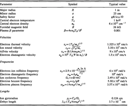
a. The TEXT tokamak. A fairly complete set of data for the fluctuation spectrum in the interior of a tokamak was obtained in the Texas Experimental Tokamak (TEXT).31 We will therefore adopt the TEXT parameters for our numerical estimates. The major radius R = 1 m, the minor radius a=25 cm, and the ratio qR/a-lO. For the electron temperature and magnetic field, we take To= 1

keVand Bo=26 kG, which represent typical experimental values. 31 In Table I we list the values of the principle pa-rameters in TEXT.

We adopt a parabolic radial profile for the equilibrium density, no(r) =n_c(

1-?-

/a2). For the equilibrium

temper-ature profile we take To(r)=T_c

Cl-?-/a

2)2, so that

7f = d In Told In no = 2 is independent of radius. The

coef-TABLE I. TEXT tokamak parameters (cgs units). Parameter

Major radius Minor radius Safety factor

Central electron temperature Central electron density Toroidal magnetic field Plasma fJ parameter Velocities 0.02

o

-0.02

o

r/a=0.5 0.2 0.4 0.6 0.8 k,.o. 1

FIG. 1. Normal mode frequency !UJ. and growth rate Yk' normalized to

\111 klJ 1 v.' as a function of the normalized poloidal wave number keP" in the midplane rla=0.5.

ficients nc and Tc are the equilibrium values of the density

and temperature at the center of the plasma, i.e., at r=O. b. The ion susceptibility. The ions will be modeled by cold fluid equations with an eddy viscosity Vi' This

viscos-ity provides the necessary sink of free energy and over-damps the unstable electron waves. The ion continuity and momentum equations are

art

_1+V·(nov.)=O

_at

I Symbol R a q To no B fJ=4rrnoToi Jil Ve= ( T aim.) 1/2 Cs= ~ToImi Typical value 1m 25 cm qRla';::!lO 1 keY 4X lOll cm-J 26 kG 0.001 (71)

Electron thermal velocity Ion sound velocity Alfven velocity

Electron diamagnetic velocity

IIA = DI( 4rrnOmi) 112

11.=108 TolVlnnollB 1.325 X 109 cm/s 3.IOX 10' cm/s 9X lOS cm/s 1.5X lOS cm/s 588 Frequencies

Electron-ion collision frequency Electron diamagnetic frequency Ion cyclotron frequency Electron bounce frequency Electron plasma frequency

Lengths

Ion gyroradius Debye length

Phys. Plasmas, Vol. 1, No.3, March 1994

_6n• 1nA vei=2.9X10 ~ (t).=keV. 0 ftj=eBlmC (t)b=velqR (t)pe= (4rrnoe2lme) 1/2 6X 104 _rad/s 106 rad/s 2.49X 108 _radls 5.30X 108 _rad/s 3.57X 1011 rad/s 0.124 cm 3.7X 1O-~ cm

1.2 0.05 1 0.04 ~ 0.8 co

'i'

0 0 :::::: 0.03 :::::: 0.6 _..., ,.\II ,.\II _iii

---

"

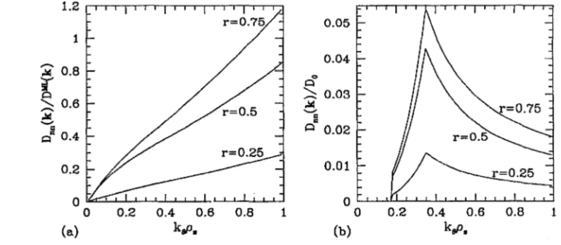
o 0.02 0" 0.4 0.2 0.01 0 0 0 0.2 0.4 0.6 0.8 1 0 0.2 0.4 0.6 0.8 (a) k,p. (b) k,p.

FIG. 2. (a) Diffusion coefficient D •• (k_e), normalized to the mixing-length estimate ~L(ke), as a function of the normalized poloidal wave number

keP" for several values of the radius ria. (b) Diffusion coefficient D •• (ke), normalized to Do, as a function of the normalized poloidal wave number

keP., for several values of the radius ria.

and

avi=~ (-VZ+~VXBo)

+v.

v

2

v.

at

mi 'f' c I I I ' (72)

where

Vi

is the ion velocity and mi is the ion mass. By taking the Fourier transforms of these equations in space and time and solving them perturbatively in the limit

lD.(fij , we find

n{ eifJ no =TOXi' with

(73) where

ri=kfvj

is an effective eddy viscosity damping, which depends on the turbulent spectrum. Note that this very simple form of the ion susceptibility does not neces-sarily reflect any direct contribution of the ions themselves to the anomalous transport. Furthermore, we assume that the ions are cold, i.e., Ti'<Te , which is usually not true, especially in the larger tokamaks.

It is known from experiments3I that the frequency spread AlDk of the fluctuations spectrum remains

compara-ble to the normal mode frequency lDk over the entire range

of relevant wave numbers, i.e., for 0.1 <k 1 Ps<.I.0. Since we assume that the ion nonlinearities are the only cause of spectrum broadening, the requirement that AlDk-lDk

im-plies a scaling

r

i=lD*/(2kI p;). (74)

Since lD* <r. k 1 , we haves3

r

(<r. kit.

The normal mode frequency and growth rate are found by solving the dispersion relation,

g> (lD,k) <r. [Xj(lD,k) -X;(lD,k)] =0,

where lD=lDk+iYk,

xf

is given by Eq. (B19) of Appendix Band X{ is given by Eq. (73). The results for lDk and Yk are

plotted in Fig. 1 as a function of ke, in the tokamak

mid-Phys. Plasmas, Vol. 1, No.3, March 1994

plane r=0.5a. Note that the damping rate Yk is about half the mode frequency lDk' in accordance with our choice for

r

i , Eq. (74).

c. The fluctuation spectrum. We assume that the fre-quency dependence of the experimental potential fluctua-tion spectrum can be represented by a simple Lorentzian profile centered on the eigenfrequency, so that

(75)

where Ik , the frequency integrated spectrum, is defined by

(76)

Note that Yk gives the half-width at half-maximum. The spectrum Ik has been measured in TEXT.3I We model the data by

(

0, if k_e

<

1.41 cm-I;

I_k=0.41 X 1, if 1.41 cm- I <k_e<2.83 cm- I; (kel2.83)-4, if k_e>2.83 cm-t •

(77) Note that we introduce a cutoff at the small wave numbers, and the constant 0.41 is chosen such that !Ik dkI(21T) 3

=

1. We have assumed isotropy in (ky,k_e), i.e., in the direction perpendicular to the magnetic field, as was also assumed in the interpretation of the experimental data.31

Finally, we use the "mixing-length" estimate of the potential fluctuation spectrum to model its radial depen-dence,

(78)

2. The diffusion coefficients

In Sec. II, we have derived general expressions for the diffusion coefficients, given by Eqs. (62)-(65). We now

2 0.8 1.5

!l

0.6 IT 'E _::s

..

_t> ~ ...

b

0.4 c::l

~

_a:! 0.5 ;; 0.2 0 0 0 0.2 0.4 0.6 0.8 0 0.2 0.4 0.6 0.8

(a) ria (b) ria

FIG. 3. (al Spatial variation of the diffusion coefficients _{Dnn , Dnr , Drn • and Drr} I nonnaIized to the mixing-length estimate JYliL. (b l Spatial variation

of the diffusion coefficients _{Dnn , Dnr , Drn} I and Drr , obtained assuming JYliL <X (rla)[l- (rla)2]2.

use the parameters described in the previous section to evaluate numerically the diffusion coefficients.

a. Wave number dependence of the diffusion coeffi-cients. In Eqs. (62)-( 65), the sum over the four-vector k, l:k> actually represents the integrals

f

dk/(2'1T)3

f

dUJ/2'1T.

The four diffusion coefficients _{Dnn, DnT • D Tn ,} and DTT

can therefore be written as

f

dk dUJ

Dab = (2'1T)3 2'1T DabCk,UJ), (79)

where Dab(k,UJ) is a diffusion coefficient per unit frequency bandwidth and wave number bandwidth. If we use Eq. (75) for the frequency spectrum, the integrations over UJ in (62 )-( 65) can be performed in the complex plane by the method of residues, closing the contour of integration in the upper-half plane. The pole of the plasma dielectric function (UJk,Yk) is in the lower-half complex plane, and does not contribute to the integral. We find

0.04 0.02

o

I=----O""!_~=::-::::-_

-_'""'_=----0.02 -0.04

o

(a) 0.2 0.4 ria 0.6 (80) 0.8 where

xr-x:-)

1 Xi-X! -iUJ

x

[(l--r)Ho+rAo]

1

. '

(81) W="'k+IYk

and similar expressions for the three other coefficients. In Eq. (81), Ik is the frequency-integrated spectrum, defined by (76). If we assume isotropy in the (kr,ko) plane, the functions Dabek) = Dab(k_O)' The mixing-length estimate of

Dnn is given by where T ~

w;

1. Therefore,

...

..

ES

_c::l 1.5 IT 1 0.5 OL...oll""""':....I--..L....JI-L-'--'-J...l...L...L...L....JI-L-'

o

0.2 (b) 0.4 ria 0.6 O.B (82)

FIG. 4. (al Contributions of the circulating electrons to the coefficients _{Dnnl Dnr • Drn , and D}TT • nonnalized to the mixing-length estimate lJ'lL. (b)

Contributions of the trapped electrons to the coefficients _{Dnn. Dnr • Drn , and Drr , nonnalized to the mixing·length estimate} JYliL.

0.8 51 0.6 Cl "-_Ii Cl 0.4 0.2

-

--. ...

_,

0~=-.l..-L.--'-.1....J.--'-.1....J.--'-.1....J.--L...1....l--'

o

0.2 0.4 0.6 0.8 (a) ria 1 0.8 51

-E:

0.6

J

0.4 "".---...

,

0.2 / ' / " / ' OL....lo<:::::L..:L-L.-1-lL-L...J...J--L.-'-l-L-.1....J.-'-l

o

0.2 0.4 0.6 0.8 (c) ria

!

~

"

Cl 51· Cl

)

1 0.8 0.6 0.4 ",....---...

,

/ ' 0.2 / ' / ' / ' 0 0 0.2 0.4 0.6 0.8 (b) ria 2 1.5 1 ,,-,,/ ,,-0.5 ,,- ,,-0 0 0.2 0.4 0.6 0.8 (d) ria

FIG. 5. (a)-(d) DIA (solid lines) and test-particle (dashed lines) results for the diffusion coefficients Dnn , DnT , DTn , and DTT , normalized to the

mixing-length estimate IJ'fL.

T 2 Z 2 .

L

(C) (

le'l'kl' \

1

nM

(k,m) ~ eB

Jil

To

1m;

(83)

and

(84)

In Fig. 2Ca), we show the diffusion coefficient _Dnn(ke) normalized to the mixing-length value IJMLCke) for vari-ous values of ria. These results are independent of our choice for the frequency-integrated spectrum Ik • In

Fig. 2(b), we show Dnn(ke)1 Do, where Do

=

0.41(cTleB)2p;2m;t. for the particular choice of Ik given in Eq. (77). The three other diffusion coefficients, namely Dnr(ke), Drn(ke), and Drr(ke) have k depen-dences very similar to that of Dnn(k_e).

h. Spatial dependence of the diffusion coefficients. The transport coefficients Dab are obtained by integrating the coefficients Dab(k) over k using (77) for I_{k ,}

Dab=

J

(:)3 Dab(k).

In Fig. 3(a), we show the coefficients DaV

nM

L, where

IJML=

J

nM

L_{(k)dkI(21T)3,}

as a function of the normalized radius ria. If we assume Eq. (78) for the radial depen-dence of the potential fluctuation spectrum,

Phys. Plasmas, Vol. 1, No.3, March 1994

nM

L_{cc2Crla)[1-(rla)2f}

In Fig. 3(b), we show the co-efficients (DaV

IJML)

X2Crla)[1-Crla)2f. All four coef-ficients have similar radial dependences. Experimentally, the heat conductivity DTT is found to increase with r near

the edge. Our result does not follow this prediction. How-ever, all the calculations presented in this work are valid in the "interior" of the tokamak plasma, not near the edge, where other physical mechanisms prevail.

0.08 0.06 0.04 0.02 0.2 0.4 0.6 0.8 ria

FIG. 6. Spectrum modulation coefficients In and IT'

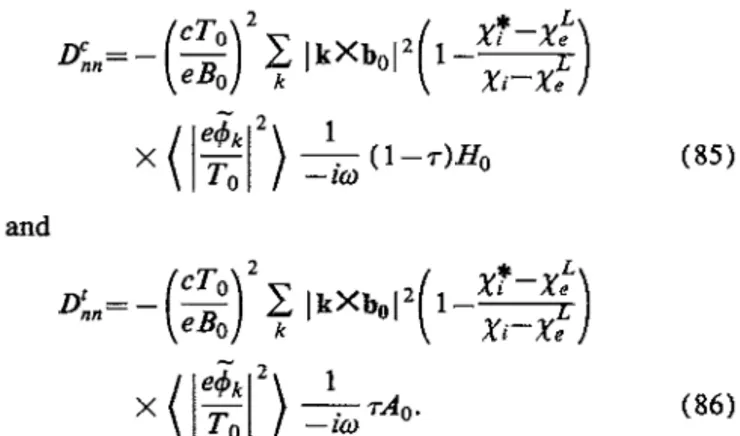
c. Relative contribution of trapped and circulating elec-trons. The diffusion coefficients Dab' given by Eqs. (62)-(65) in Sec. II can be written as the sum of two compo-nents, representing the contributions of the trapped and circulating electrons. For example, Dnn can be written as Dnn=U,tn+D~n with

If.. = _ (CTo)2

I

IkXb 12(1

xr-x~)

nn eBo k

°

xi-xf

X

(r!:I)

~iW

(l-r)Ho (85) and

(86)

In Figs. 4(a) and 4(b), we show the contributions from the trapped and the circulating electrons to the coef-ficient Dnn/ JjML. The contribution from circulating trons is very small compared to that of the trapped elec-trons, even though the numbers of circulating electrons and trapped electrons are comparable in the midplane of the tokamak (r -

iii

= ~2r/R = 0.5; cf. Appendix A), and there are much more circulating electrons than trapped electrons at r/a=0.1(1-r-0.8). Therefore the analysis of the problem could be simplified by considering adiabatic circulating electrons. This has been pointed out for quasilinear calculations as well. 84

Note that all the diffusion coefficients are positive (cf. Fig. 3). The contribution from the circulating electrons to the off-diagonal diffusion coefficients DnT and _{D Tn} is neg-ative, whereas the contribution from the trapped electrons is positive. Since the trapped electrons dominate, the off-diagonal diffusion coefficients are positive. It has been sug-gested that the negative off-diagonal diffusion coefficients obtained in calculations involving only circulating elec-trons could explain the "inward" convective motion ob-served in modulation experiments. However, as we have shown here, the presence of even a very small population of trapped electrons is sufficient to guarantee the positivity of all four diffusion coefficients.

d. Comparison with test-particle results. The function Dnn is given by Eq. (62), obtained from our DIA calcula-tions. The test-particle result is recovered by dropping the

(v'1C/w",)

J

[dk/(21T)3} (dw/21T)

(I

e~k/ToI2) where

term proportional to lI(Xi-X;) in this expression. In Fig. 5 we compare the DIA and test-particle (TP) results for Da~JjML.

The diffusion coefficients calculated by the DIA are larger by a factor 2-4 than those obtained in the TP ap-proximation. The disagreement between the two methods is largest for _{D Tn ,} breaking the Onsager symmetry in the DIA result.

e. Onsager relations. Systems that are out of equilib-rium generally return to the equilibequilib-rium state through a variety of irreversible transport processes. Onsager8S,86

de-rived "reciprocal relations" connecting the corresponding transport coefficients. These relations reflect, on the mac-roscopic level, the time reversal invariance of the micro-scopic equations of motion. For example, a particle density gradient can cause a heat current, and a temperature gra-dient can cause a particle current. The transport coeffi-cients for the two processes are equal. The entropy produc-tion (due to the irreversible processes occurring in the system) is a bilinear expression in the fluxes and thermo-dynamic forces. The calculation of the entropY production therefore provides a way of finding the proper "conjugate" irreversible fluxes and thermodynamic forces necessary for the establishment of the phenomenological equations whose coefficients obey the Onsager relations.

From Fig. 3, we note that the two off-diagonal coeffi-cients of our transport matrix, D nT and _{D Tn ,} are not equal, i.e., the Onsager symmetry observed in quasilinear and test-particle results is not present here. This is not under-stood at present, but has been observed in other studies of anomalous transport.87,88 One difficulty is to find the "cor-rect" conjugate fluxes and forces. In particular, we have not been able to find an expression for the entropy produc-tion in the complex system studied here. It is possible that Onsager symmetry should not be expected in the case of anomalous transport, but this remains to be explained.

3. The spectrum modulation

In Sec. II, we have calculated the spectrum modulation produced by perturbations in density and temperature, and the result was written as

ik,ko Vno VTo

- 2 In(w,k_e) -+IT(w,k_{e) - ,} (87)

< 1 etPklTo I > no To

where In(w,k_e) and I r(w,k_e) are given by (69) and (70). If we integrate these results over the frequency and wave number, we obtain

(88)

J

[dkI(21T)3] (dw/21T)

(I

e~k/ToI2>Re{[ (keP-S)/(Xi-X;)] (w",/ -iw) [(l-r)Ho+rAon

In= f[dk/(21T)3](dw/21T)(

I

e~k/ToI2)

(89)

and