BLIND SOURCE SEPARATION TECHNIQUES FOR MODAL
ANALYSIS: EXPERIMENTAL DEMONSTRATION
F. Poncelet1, G. Kerschen1, JC. Golinval1, D. Verhelst2
1 University of Liège
Aerospace and Mechanical Engineering Department (LTAS) Institut de Mécanique et de Génie Civil (B52/3)
Chemin des Chevreuils 1 B-4000 Liège 1
Belgium
2 Techspace Aero (Safran Group)
Liège, Belgium
SUMMARY: The present study carries out output-only modal analysis using two blind source separation (BSS)
techniques, namely independent component analysis and second-order based identification. It is shown under which circumstances the normal coordinates of the vibration modes may be interpreted as virtual sources, which renders the application of these BSS techniques possible. To support the theoretical findings, numerical experiments are first carried out using a discrete system of three masses. Secondly the method is applied to a real-life structure which is a blade extracted from a turbojet engine stator. The results are compared with the stochastic subspace identification method.
KEYWORDS: Blind source separation, system identification, modal analysis, independent component analysis, second-order blind identification
1. INTRODUCTION
Blind source separation (BBS) techniques were initially developed for signal processing in the early 1980s [1]. The general aim of BSS techniques is to recover unobserved source signals from their observed mixtures. The well-known problem named cocktail-party problem perfectly illustrates this idea. It consists in retrieving the initial speech signals emitted by several persons speaking simultaneously in a room using only the mixed signals which are recorded by a set of microphones located in the room.
The BSS techniques quickly found many applications in speech processing and wireless communications and proved useful for the analysis of multivariate data sets such as financial time series [2], astrophysical data sets [3], image processing [4], electrical and hemodynamic recordings from the human brain [5]. The mechanical engineering community recently took into consideration these techniques, in areas such as non-destructive control, online condition monitoring or noise analysis.
This paper investigates the usefulness of BSS techniques for modal analysis through the virtual source concept [6]. Indeed, the sources considered herein are not the physical excitations of the identified structure, which allows us to interpret the response of a mechanical system as a static mixture of (virtual) sources. Two methods are considered, namely independent component analysis (ICA) [7] and second-order based identification (SOBI) [8]. A simple numerical application (a three-degree-of-freedom system) firstly illustrates the proposed methodology. Secondly the algorithms are applied to a real-life structure to demonstrate the applicability of the
methodology for practical applications. A comparison with the stochastic subspace identification (SSI) method [9] is finally achieved.
2. THEORETICAL BACKGROUND
This section briefly introduces the two considered algorithms (ICA and SOBI) and shows that they can be useful for modal identification, even in the absence of external forces. However, the detailed description of these algorithms is beyond the scope of this paper. The reader may consult [7, 8, 10] for further details.
2.1. Two considered BSS algorithms
The objective of SS techniques consists then in revealing the underlying structure hidden in a set of measured data. The simplest BSS model assumes the existence of n source signals and the observation of as many mixtures . We focus on linear and static mixtures for which BSS is well established. Mathematically, this can be expressed as in equation
( ) ( ) 1 , , n s t …s t ( ) ( ) 1 , , n x t … x t
(1), where A is referred to as the mixing matrix.
(1)
( )t = ⋅ ( )
x A s t
The basic idea of BSS is to recover the unobserved source signals s t( ) from their observed mixtures x t . ( )
Blind means that very little, if anything, is known about the mixing matrix , and that fairly general assumptions are made about the source signals.
A
2.1.1. Independent Component Analysis
To alleviate the lack of a priori knowledge about the mixture, ICA assumes that the observed data are linear combinations of statistically independent sources. Since it is usually not possible to estimate sources that are perfectly statistically independent and since noise often perturbs the measurements, ICA consists in searching a linear transformation that minimizes the statistical dependence between its components. The method considered here is based on the mutual information concept and maximizes the non-Gaussianity of the sources. Statistical independence and non-Gaussianity are the guiding principles of ICA [10]. More explanations are also available in [11, 12].
2.1.2. Second-Order Based Identification
The objective of the SOBI algorithm is to take advantage, whenever possible, of the temporal structure of the sources for facilitating their separation [8]. SOBI is therefore an interesting alternative to ICA for sources with different spectral contents, which is often the case in structural dynamics [12].
SOBI is based on the joint diagonalization of several matrices and can be interpreted as an extension of the POD method [13] for a set of covariance matrices characterized by different time lags. These matrices are evaluated from the observed data x t , and the idea is to find a unitary matrix, which jointly diagonalizes all the ( )
covariance matrices. It can be proven that this unitary matrix corresponds to the mixing matrix. Another advantage of the procedure is that being based on the joint diagonalization of a set of covariance matrices it only involves second-order statistics, which are easier to compute.
2.2. Application for Modal Analysis
In view of the BSS techniques success, some attempts were performed to use them in the field of structural dynamics. They were generally based on equation (2), which expands the response of a mechanical system (governed by the equation of motion (3)) in terms of a convolutive product between the impulse response and the external forces f . Unfortunately the application of ICA to a convolutive mixture of sources is not yet completely solved and raises several problems [14]. Moreover the prime goal in this case is to separate all the (physical) excitations applied on the structure.
h (2) ( )t = ( )t ⊗ ( ) x h f t t (3) ( )t + ( )t = ( ) Mx Kx f
The use of BSS techniques for modal analysis requires the introduction of the virtual source concept. Indeed, besides expression (2), the response of system (3) can also be expanded in terms of normal modes and normal coordinates
( )i
n
i
η using a static product as follows
(4) ( ) ( ) ( ) ( ) 1 m i i i t t = =
∑
⋅ = ⋅ x n η N η t tBy definition, the normal modes provide a complete set for the expansion of an arbitrary vector. It turns out that the normal coordinates act as virtual sources on the system regardless the number and the type of the physical excitation forces. Under the assumption of independent normal coordinates, the application of BSS methods should therefore provide a straightforward identification of the eigenmodes of a structure through the computed mixing matrix (5). For further theoretical development, the reader can consult [11, 12].
and
=
N A η( )t = s( ) (5)
3. NUMERICAL APPLICATIONS
Numerical tests were performed in order to evaluate the proposed methodology and to compare the two algorithms considered in this paper. Only the main results are summarized here, the complete analysis (on discrete and distributed-parameter systems) was detailed in [15].
3.1. System Description
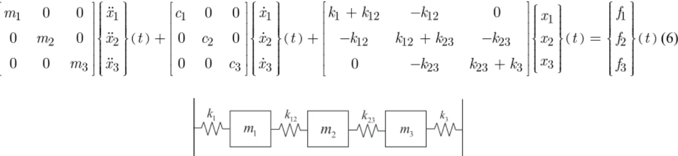
The system considered herein is a discrete (three-degree-of-freedom) system which is depicted in Figure 1. Diagonal damping is added to the system. The equations of motion are
( ) ( ) 1 12 12 1 1 1 1 1 2 2 2 2 12 12 23 23 2 3 3 3 3 3 23 23 3 0 0 0 0 0 0 0 0 0 0 0 0 0 0 k k k x x m c x m x t c x t k k k k x x m x c x k k k ⎡ ⎤ ⎧ ⎫ ⎧ ⎫ ⎡ ⎤⎪⎪ ⎪⎪ ⎡ ⎤⎪⎪ ⎪⎪ + − ⎪⎧ ⎪⎫ ⎢ ⎥ ⎢ ⎥⎪ ⎪ ⎢ ⎥⎪ ⎪ ⎢ ⎥⎪⎪ ⎢ ⎥⎪⎪ ⎪⎪ +⎢ ⎥⎪⎪ ⎪⎪ + − + − ⎪ ⎨ ⎬ ⎨ ⎬ ⎢ ⎥⎨ ⎬ ⎢ ⎥⎪ ⎪ ⎢ ⎥⎪ ⎪ ⎪ ⎢ ⎥ ⎢ ⎥⎪ ⎪ ⎢ ⎥⎪ ⎪ ⎪ ⎪ ⎪ ⎪ ⎪ ⎢ ⎥⎪ ⎢ ⎥⎪⎪ ⎪⎪ ⎢ ⎥⎪⎪ ⎪⎪ − + ⎪⎩ ⎣ ⎦⎩ ⎭ ⎣ ⎦⎩ ⎭ ⎣ ⎦ ( ) ( ) 1 2 3 f t f t f ⎧ ⎫ ⎪ ⎪ ⎪ ⎪ ⎪ ⎪ ⎪ ⎪ ⎪ ⎪ ⎪ = ⎨ ⎬⎪ ⎪ ⎪ ⎪ ⎪ ⎪ ⎪ ⎪ ⎪ ⎪ ⎪ ⎪ ⎪ ⎪ ⎭ ⎪ ⎪⎩ ⎭ (6) 1 m m2 m3 1 k k12 k23 k3
Figure 1 – Schematic of the 3 dof system
The system response is computed using Newmark’s algorithm with a sampling frequency of 100 Hz. It is then
resampled to 10 Hz. The system parameters are , and and
for the mass and stiffness parameters. Diagonal damping is introduced using only one parameter, denoted α. This gives , and finally .
1 2 m = m =2 1 m =3 3 1 12 23 3 1 k =k =k =k = 1 1 c =α⋅m c2 =α⋅m2 c3 =α⋅m3
3.2. Modal Parameters Identification using BSS
The proposed modal analysis process can be summarized as below:
1. Perform experimental measurements of the structure response (or simulate it) to obtain time series at different sensing positions.
2. Apply the BSS techniques to the measured time series to estimate the mixing matrix and the sources .
A
( )t
s
3. The mode shapes are contained in the mixing matrix A.
4. The identification of the corresponding natural frequencies and damping ratios is straightforward using 1-dof fitting techniques applied to the normal coordinates.
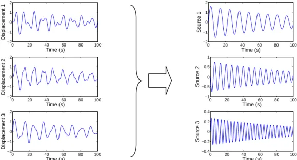
Figure 2 illustrates this methodology for the free response of the 3-dof system. The considered initial conditions are zero except for x3( )0 = 1. The left column corresponds to the simulated system response x t for the i( )
three masses. These data are the only information furnished to the BSS algorithm. On the right side are presented the identified sources. They correspond to the normal coordinates of the system. The natural frequencies and damping ratios can be evaluated from these time series.
0 20 40 60 80 100 −2 −1 0 1 2 Time (s) Displacement 1 0 20 40 60 80 100 −2 −1 0 1 2 Time (s) Source 1 0 20 40 60 80 100 −2 −1 0 1 2 Time (s) Displacement 2 0 20 40 60 80 100 −1 −0.5 0 0.5 1 Time (s) Source 2 0 20 40 60 80 100 −2 −1 0 1 2 Time (s) Displacement 3 0 20 40 60 80 100 −0.4 −0.2 0 0.2 0.4 Time (s) Source 3
Figure 2 – Simulated responses for the 3-dof system (on the left) and normal coordinates after SOBI application (on the right)
3.3. ICA/SOBI comparison
Using the same 3-dof system, a comparison of the two methods (ICA and SOBI) was achieved regarding measurement noise and the level of damping. The theoretical modal parameters (namely the mode shapes, natural frequencies and damping ratios) are calculated by solving an eigenvalue problem, and the theoretical normal coordinates are computed using (7).
( ) 1 ( )
th t = Nth− x t
η (7)
The modal assurance criterion (8) is used to assess the accuracy of the mode identification.
{ }
(
)
(
)(
)
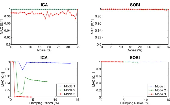
2 , T BSS th BSS th T T BSS BSS th th MAC n n = n n n n n n (8)The results of this study are summarized in the 4 plots below for the three identified modes. The left and right columns correspond to the ICA and SOBI algorithms, respectively.
To investigate the robustness of the proposed algorithms to noise, the displacement signals are corrupted by non-Gaussian random noise (uniform distribution) after the Newmark simulation. The noise RMS amplitude is gradually increased from 0 to 35 % of the signal RMS value. Results seem to be fairly insensitive to noise. The free response of the damped system for values of α ranging from 0 to 0.15 is also considered. This latter value corresponds to a highly damped system; the damping ratios of the three modes are 13.33%, 8.18% and 4.73%, respectively. Both methods perform well for the weakly damped system. When damping increases beyond 1%, the correspondence between the ICA modes and the vibration modes is no longer valid, whereas the SOBI method continues to provide accurate results.
To conclude this numerical study, let us notice that this methodology is also applicable to forced responses. The conclusions are similar. More details may be found in [12, 15].
0 5 10 15 20 25 30 35 0.9 0.92 0.94 0.96 0.98 1 ICA Noise (%) MAC [0,1] 0 5 10 15 20 25 30 35 0.9 0.92 0.94 0.96 0.98 1 SOBI Noise (%) MAC [0,1] 0 5 10 15 0 0.2 0.4 0.6 0.8 1 ICA Damping Ratios (%) MAC [0,1] Mode 1 Mode 2 Mode 3 0 5 10 15 0 0.2 0.4 0.6 0.8 1 Damping Ratios (%) MAC [0,1] SOBI Mode 1 Mode 2 Mode 3
Figure 3 – Robustness of ICA and SOBI with respect to noise and damping level.
4. EXPERIMENTAL DEMONSTRATION
As mentioned in the introduction, this paper is dedicated to the application of BSS techniques for modal identification in practical applications. This section applies the SOBI algorithm to a real-life-structure, and the stochastic subspace identification method [9] is used as reference to check the results validity.
4.1. Setup Description
The real-life structure which is considered is a stator blade extracted from a turbojet engine. The blade was tested in a clamped-free configuration with the blade root clamped in a vice as shown in Figure 4. The 15 considered measurement locations are also presented on the picture. A hammer provided a short impulse to the system, and non-contact vibration measurements were performed using a laser vibrometre. This avoids to perturb the structure with the mass of sensors but forbids simultaneous measurements.
Figure 4 - Experimental fixture
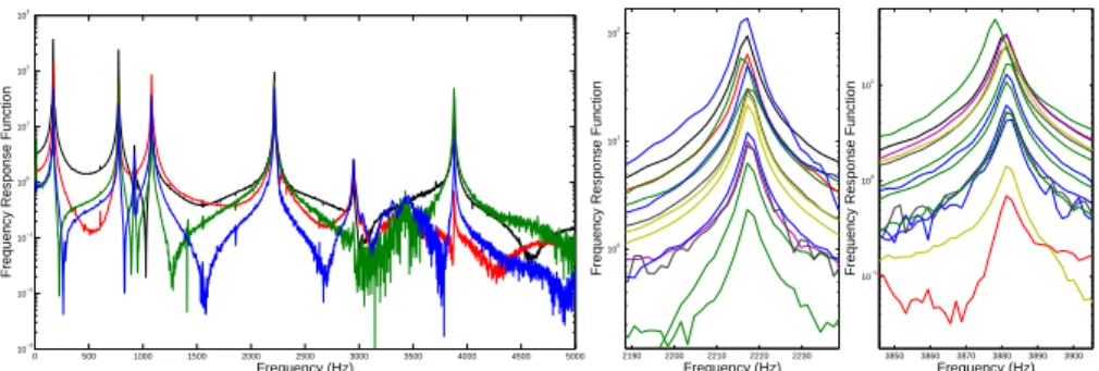
The receptance frequency response functions (FRFs) were recorded in the range [0 − 5000] Hz; some of them are plotted in Figure 5. This figure reveals the presence of 6 natural frequencies around 170, 780, 1080, 2220, 2950 and 3880 Hz, respectively. A finite element model of the structure was created and also confirmed the presence of 6 resonant frequencies in this frequency range.
In order to perform a modal identification, a set of 15 impulse response functions was computed by applying the inverse Fourier transform to the measured FRFs. As we can observe on the two right graphs which depict zooms around two eigenfrequencies, there is a slight frequency shift between the FRFs. This frequency shift is equal to the frequency resolution of the measurements and probably takes its origin in the fact that the FRFs were not acquired simultaneously. This will lead to a splitting of these modes (see below).
0 500 1000 1500 2000 2500 3000 3500 4000 4500 5000 10−3 10−2 10−1 100 101 102 103 Frequency (Hz)
Frequency Response Function
2190 2200 2210 2220 2230 100
101
102
Frequency (Hz)
Frequency Response Function
3850 3860 3870 3880 3890 3900 10−1
100
101
Frequency (Hz)
Frequency Response Function
Figure 5 – Frequency response functions of the clamped blade.
4.2. Modal Analysis using Stochastic Subspace Identification Method
In the field of output-only modal analysis, the stochastic subspace identification (SSI) method is well-known and can be considered as a mature method. The used version is based on the covariance-driven algorithm. The resulting stabilization diagram, presented in Figure 6, confirms the presence of 6 natural frequencies. However, close-ups of the stabilization diagram show that two stabilized poles, related to a single physical mode, are present around 2220 (second torsional blade mode) and 3880 Hz (third torsional blade mode). The modes in closer correspondence with the expected modal forms are therefore retained, and the others are discarded.
0 500 1000 1500 2000 2500 3000 3500 4000 4500 5000 0 5 10 15 20 25 30 Frequency (Hz) System order 22100 2215 2220 2225 2230 5 10 15 20 25 Frequency (Hz) System order 38700 3875 3880 3885 3890 5 10 15 20 25 Frequency (Hz) System order
Figure 6 – Stabilization diagram for the SSI method.
4.3. Modal Analysis using SOBI
The SOBI-based modal analysis method is now applied to the blade experiment. Because there are 15 measurement locations, a total of 15 virtual sources can be considered. Two of the 15 sources are presented in Figure 7. 0 0.1 0.2 0.3 0.4 −1 −0.5 0 0.5 1 Source 2 Time (s) 0 0.1 0.2 0.3 0.4 −0.5 0 0.5 Source 6 Time (s) Figure 7 – Two identified sources (numbered #2 and #6)
4.3.1. Source Selection Criterion
The number of identified sources being higher than that of the structural modes, the actual sources have to be selected. The selection is greatly facilitated by computing the error realized during the fitting of the time series of the sources with exponentially damped harmonic functions. Indeed, in case of viscous damping, the generic expression of the normal coordinates is (9) where and ξ are the natural pulsation and the damping ratio of the mode, respectively.
ω
Figure 8 depicts the fitting error for each identified source. Seven sources have a fitting error below 4%, and the source #11 has a somewhat higher error, 16%, but it corresponds to the mode around 2900 Hz which has the lowest participation in the system response (see Figure 5). The remaining sources have their error above 50%. This indicates that sources #2, #4, #6, #8, #9, #11, #12 and #13 can be safely selected.
( )t A exp( t) cos
(
1 2 tη = ⋅ −ξω ⋅ −ξ ω +α
)
(9)For the same reason as for the SSI method (splitting of the second and third torsional modes), sources #9 and #13 are not taken into account.
2 6 4 9 13 8 12 11 10 7 3 5 1 14 15 0 10 20 30 40 50 60 70 80 90 100 Source number Fitting error (%)
Figure 8 – Fitting error of the identified SOBI sources
4.3.2. Comparison with SSI
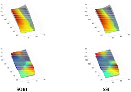
We can now compare results issued from SSI and SOBI identifications. Figure 9 presents the comparison of 2 modes identified using SSI and SOBI. The visual similarity is obvious. In order to numerically evaluate the correspondence, the MAC matrix is computed between SSI and SOBI modes. A comparison is also carried out with the eigenmodes computed using the finite element method (see Figure 10). All these results confirm that an accurate and consistent identification is carried out using SOBI. The ICA algorithm was also applied and compared with the SSI results. All the modes were not caught in this case.
Mode 2 775 Hz
Mode 5 2950 Hz
SOBI SSI
Figure 9 – Picture of two eigenmodes computed using SSI and SOBI
1/170 2/775.4 3/1080.7 4/2216.6 5/2949.8 6/3878.2 1/170.1 2/775.4 3/1081.4 4/2217.4 5/2949.6 6/3880.1 Modes SOBI Modes SSI 0.97 0.97 0.97 0.94 0.94 0.96 0.1 0.2 0.3 0.4 0.5 0.6 0.7 0.8 0.9 1/171.9 2/774 3/1071.9 4/2202.1 5/3089.6 6/3878.5 1/170 2/775.4 3/1080.7 4/2216.6 5/2949.5 6/3878.2 Modes FE Modes SOBI 0.98 0.99 0.96 0.68 0.90 0.84 0.1 0.2 0.3 0.4 0.5 0.6 0.7 0.8 0.9 1/170.1 2/775.4 3/1081.4 4/2217.4 5/2949.6 6/3880.1 1/169.4 2/776 3/1082.2 4/2215.7 5/2948.6 6/3876.9 ModesSSI ModesICA 0.97 0.94 0.96 0.95 0.51 0.1 0.2 0.3 0.4 0.5 0.6 0.7 0.8 0.9
5. CONCLUSIONS
This study applies BSS techniques, and particularly the SOBI algorithm, to the measured responses of mechanical systems. An output-only modal analysis technique is developed, based on an existing relationship between the vibration modes and the so-called mixing matrix. For the SOBI method, this relation holds as well for weakly as moderately damped systems.
Even if further research is needed for the analysis of complex industrial structures, the numerical and experimental applications considered herein show that the method holds promise in the area of system identification:
1. A truly simple identification scheme is proposed, because the straightforward application of SOBI to the measured data yields the modal parameters.
2. According to the numerical simulations carried out herein, the method is fairly insensitive to the presence of measurement noise.
3. A seemingly robust criterion has been developed for the selection of the actual modes. This is useful when the number of sources exceeds the number of active modes. Compared to standard modal analysis techniques, the use of stabilization charts, which always require a great deal of expertise, is therefore avoided.
A potential limitation of the method is that sensors should always be chosen in number greater or equal to the number of active modes. Note that the application of the method to forced (random) response was also tested [12] and leads to the same conclusions. The determination of the modal parameters and the selection criterion are then realized using the random decrement method [16, 17] to obtain the free response from the identified sources. This will be address in a subsequent study [18].
ACKNOWLEDGEMENTS
The authors are grateful to Pierre Comon for making his ICA codes freely available at http://www.i3s.unice.fr/~comon/. The authors are also grateful to Jean-Francois Cardoso for making his extended Jacobi technique available at http://www. tsi.enst.fr/~cardoso/jointdiag.html. The author F. Poncelet is supported by a grant from the Walloon Government (Contract No 516108 — VAMOSNL). The author G. Kerschen is supported by a grant from the Belgian National Fund for Scientific Research (FNRS). The authors would like to thank Maxime Peeters for his assistance in the experimental part of this study.
6. REFERENCES
1. Antoni, J. and S. Braun, Special issue on blind source separation: editorial. Mechanical Systems and Signal Processing, 2005. 19: p. 1166-1180.
2. Back, A.D. and A.S. Weigend, A First Application of Independent Component Analysis to Extracting
Structure from Stock Returns. International Journal of Neural Systems, 1997. 8.
3. Patanchon, G., J. Delabrouille, and J.-F. Cardoso, Source separation on astrophysical data sets from the
WMAP satellite. Computer Science, 2004. 3195: p. 1221-1228.
4. Hyvärinen, A. and E. Oja, Independent Component Analysis: Algorithms and Applications. Neural Networks, 2000. 13(4-5): p. 411-430.
5. Juang, J.S. and R.S. Pappa, An eigensystem realization algorithm for modal parameter identification
and model reduction. Control and Dynamics, 1985. 12: p. 620-627.
6. Jung, T.P., et al. Imaging brain dynamics using independent component analysis. in IEEE. 2001. 7. Comon, P., Independent component analysis: a new concept? Signal Processing, 1994. 36: p. 287-314.
8. Belouchrani, A., et al., A blind source separation technique using second order statistics. IEEE Transactions on Signal Processing, 1997. 45(2).
9. Van Overschee, P. and B. De Moor, Subspace Identification for Linear Systems: Theory,
Implementation, Applications. 1996: Kulwer Academic Publishers.
10. Hyvärinen, A., J. Karhunen, and E. Oja, Independent Component Analysis, ed. S. Haykin. 2001: John Wiley & Sons, Inc. 481.
11. Kerschen, G., F. Poncelet, and J.-C. Golinval, Physical interpretation of Independent Component
Analysis in structural dynamics. Mechanical Systems and Signal Processing. available online on
www.science-direct.com.
12. Poncelet, F., G. Kerschen, and J.-C. Golinval, Output-only modal analysis using blind separation
13. Kerschen, G., et al., The method of proper orthogonal decomposition for dynamical characterization
and order reduction of mechanical systems: an overview. Nonlinear Dynamics, 2005. 41: p. 147-170.
14. Antoni, J., Blind separation of vibration components : Principles and demonstrations. Mechanical
Systems and Signal Processing, 2005. 19: p. 1166-1180.
15. Poncelet, F., G. Kerschen, and J.-C. Golinval. Experimental modal analysis using blind source
separation techniques. in International Conference on Noise and Vibration Engineering (ISMA). 2006.
Leuven.
16. Asmussen, J.C., Modal analysis based on the random decrement technique: Application to civil engineering structures, in Department of Building Technology and Structural Engineering. 1997,
University of Aalborg: Aalborg.
17. Cole, H.A., On-The-Line Analysis of Random Vibrations. AIAA Paper, 1968. 68(288).
18. Poncelet, F., G. Kerschen, and J.-C. Golinval. Blind Source Separation Techniques - Another Way of
Doing Operational Modal Analysis. in International Operational Modal Analysis Conference. 2007.