Attitude estimation of an artillery shell in free-flight from accelerometers and magnetometers

(1)

HAL Id: tel-03097354

https://pastel.archives-ouvertes.fr/tel-03097354

Submitted on 5 Jan 2021

HAL is a multi-disciplinary open access

archive for the deposit and dissemination of sci-entific research documents, whether they are pub-lished or not. The documents may come from teaching and research institutions in France or

L’archive ouverte pluridisciplinaire HAL, est destinée au dépôt et à la diffusion de documents scientifiques de niveau recherche, publiés ou non, émanant des établissements d’enseignement et de recherche français ou étrangers, des laboratoires

Attitude estimation of an artillery shell in free-flight

from accelerometers and magnetometers

Aurelien Fiot

To cite this version:

Aurelien Fiot. Attitude estimation of an artillery shell in free-flight from accelerometers and magne-tometers. Automatic Control Engineering. Université Paris sciences et lettres, 2020. English. �NNT : 2020UPSLM039�. �tel-03097354�

(2)

Préparée à MINES ParisTech

Estimation en vol de l'attitude de projectiles à l'aide

d'accéléromètres et de magnétomètres

Attitude estimation of an artillery shell in free-flight from

accelerometers and magnetometers

Soutenue par

Aurélien FIOT

Le 30 Octobre 2020

École doctorale no₆₂₁

Ingénierie des Systèmes,

Matériaux, Mécanique,

En-ergétique

Spécialité

Mathématique et

Automa-tique

Composition du jury : Pascal MORIN

Pr., Sorbonne Université, ISIR Rapporteur,

prési-dent du jury

Hélène PIET-LAHANIER

Directrice scientique adjointe, ONERA Rapporteur

Tarek HAMEL

Pr., Université de Nice, I3S Examinateur

Sihem TEBBANI

Pr., CentraleSupelec, LSS Examinateur

Sébastien CHANGEY

Dr., Institut Saint-Louis Examinateur

Nicolas PETIT

(3)

(4)

Abstract

The thesis addresses the estimation of the attitude of an artillery shell in free flight, during the flight phase called exterior ballistics. Attitude estimation is an essential step for the development of « smart-shells » a.k.a. « guided-ammunition » which are capable of achieving various guidance tasks such as in-flight re-targeting and optimization of range. The method developed here uses strapdown accelerometers and magnetometers only. In particular, it does not use any rate gyro, a pricey component that is too fragile to sur-vive the stress of gunshot when it is not subjected to import restrictions. For attitude determination, we circumvent the intrinsic inability of accelerome-ters to provide direction information in free flight, by employing them not to measure the direction of gravity but to estimate the velocity w.r.t. the air. This is achieved through a frequency detection method applied to the pitch-ing and yawpitch-ing rotational dynamics generated by aerodynamics moments. In turn, the variation of the velocity gives us an orientation information that complements the direction given by the 3-axis Magnetometer. The two in-formation are treated by an attitude observer adapted from the well-known complementary filter. This adaptation requires special care and an analysis of the convergence of the resulting observer is provided. The applicability of the method is shown on simulations and real-flight experiments.

(9)

(10)

Résumé

Cette thèse présente une méthode pour estimer l’attitude d’un projectile en vol à partir de mesures de directions. L’estimation d’attitude est une étape essentielle pour le développement de « munitions intelligentes », rendant pos-sible le changement de cible en vol et l’optimisation de la portée. La méth-ode que nous proposons repose exclusivement sur un accéléromètre et un magnétomètre embarqués. En particulier, elle ne requiert pas de gyroscope, capteur coûteux et trop fragile pour survivre aux conditions de tir, quand il n’est pas soumis à des restrictions d’importation. Pour la détermination de l’attitude du projectile, nous contournons l’incapacité des accéléromètres à donner une mesure de direction de la gravité en vol ballistique, en les util-isant pour estimer la vitesse du projectile par rapport à l’air. Ceci est réalisé grâce à une méthode de détection de fréquence appliquée aux oscillations de précession et de nutation du projectile induites par les moments aérody-namiques qu’il subit. Par la suite, les variations de la vitesse du projectile nous donnent une information d’orientation partielle qui complète la direc-tion donné par le magnétomètre 3-axes. Les deux informadirec-tions sont traitées par un observateur d’attitude adapté du filtre complémentaire ; cette adap-tation n’est pas triviale et on réalise une étude détaillée de la convergence de l’observateur proposé. L’eﬃcacité de la méthode est illustrée par des résultats sur des données de simulation et des données de vol réel.

(11)

(12)

Remerciements

A Nicolas, directeur impliqué, prodigue en conseils avisés et bienveillant. Ce fut un plaisir de travailler avec lui, et cette thèse lui doit énormément.

A Sébastien, pour son accompagnement, sa grande disponibilité, et égale-ment pour son accueil lors des (brèves) séquences alsaciennes de ce doctorat. A Christophe, avec qui il était toujours un plaisir de discuter, et à qui je dois de nombreuses pistes de recherche.

A Pascal Morin et Hélène Piet-Lahanier, rapporteurs de ce manuscrit, pour le temps qu’ils y ont consacré et leurs précieux retours. Aux autres membres du jury, avec qui j’ai eu également plaisir à échanger.

A l’école des Mines et au Centre Automatique et Systèmes, pour ces an-nées passées à y travailler, à y enseigner et à y vivre. Professeurs, co-thésards et étudiants ont fait de ce doctorat une expérience bien moins solitaire qu’on ne me l’avait décrit. J’espère que cette ambiance toute particulière y perdur-era encore longtemps. Merci aux anciens (Florent, Delphine, Pauline, Jean, Charles-Henri, Pierre, Naveen), et courage aux suivants (Matthieu, Dilshad, Loris, Hubert, Mona, Nils, Pierre-Cyril)

A Marin, Baptiste et Arnaud, à Sabine et à ma mère, pour leur soutien précieux au moment fatidique ; plus généralement à ma famille et mes amis, pour leur présence et leur patience, dans les moments de joie comme dans les moments de doute.

(13)

(14)

Chapitre 1 - Résumé

Ce chapitre introductif pose les bases du problème qui nous a intéressé au cours de cette thèse, et donne des éléments de contexte sur les munitions intelligentes d’une part, et l’estimation d’attitude en général d’autre part. On justifie le rôle central de l’attitude pour la navigation, en illustrant sa nécessité pour le guidage terminal et des applications de télémétrie. Enfin, on introduit brièvement la solution proposée, en la décomposant en plusieurs schémas-blocs : estimation fréquentielle de la vitesse d’une munition, esti-mation de l’angle de pente de la munition à partir d’une mesure de vitesse, estimation d’attitude à l’aide de la connaissance d’un angle, et finalement reconstitution d’une méthode complète reposant exclusivement sur des cap-teurs embarqués.

(15)

(16)

Chapter 1

Context and problem

statement

1.1 Introduction

The topic under consideration in this thesis is the estimation of the attitude of an artillery shell in free flight, during the flight phase termed exterior bal-listics. As will be described below, attitude estimation is an essential factor for the development of « smart-shells » or « guided-ammunition » which are capable of achieving various guidance tasks such as in-flight re-targeting and optimization of range. Lately, these topics have been of interest as signif-icant performance improvements are expected from smart-shells compared to currently employed ammunition [30, 81, 105].

The attitude estimation problem belongs to the vast class of state esti-mation problems for Six-Degrees-of-Freedom (6-DOF) rigid bodies subjected to aerodynamics eﬀects using embedded sensors. As is very common now, many rigid bodies can be equipped with low-cost strapdown inertial sen-sors, see e.g. [84, 4, 98, 26, 104, 21, 43, 27, 95, 9, 67, 68, 48], to reliably solve navigation problems, at the expense of reasonably complex on-board calculations and oﬀ-line tasks such as multi-sensor system calibration [40]. Numerous experiments have been reported in the literature for unmanned aerial vehicles [73, 49, 10, 51, 47], unmanned ground vehicles [86], micro-satellites [94, 62, 90], sounding rockets [5], spacecrafts [75, 59, 62, 90, 89, 88], smart objects [54, 18] among others. Commonly considered sensors are the component of an inertial measurement unit (IMU) : 3-axis Accelerometer, 3-axis Magnetometer and rate gyro (and sometimes GPS which is usually discarded as it is easily subjected to spoofing and jamming, especially in military applications).

(17)

ap-proach. The trajectory of a shell has a short duration due to its high speed1, and, most importantly, is often subjected to a very high spin rate [72, 103, 18, 20, 36], usually favored due to its stabilizing eﬀect on the center of mass trajectory. In practice, the spin rate saturates most low-cost rate gyro and even medium-cost ones [3]2, if they are not damaged by the high impact caused by the gunshot, of approximately 20000 G.

Attitude estimation of a rigid body is a far-reaching question in numerous fields of engineering and applied science, especially those including motion control. Classically (see e.g. [27]), following the formulation of the famous « Wahba » problem [101], two vectors measurements, usually assumed to be obtained using accelerometers and magnetometers, are suﬃcient to alge-braically (and unambiguously) reconstruct the attitude of a rigid body. The vastly documented methods to solve Wahba’s problem (see [4, 85]) have been improved in many applications with multi-sensor data fusion, adding rate gyro to the set of sensors, most frequently using Kalman filtering (see e.g. [98]) or, more recently, complementary filtering as in [67, 68, 66]. This last solution is appealing because of its simplicity of implementation (re-lying on a few nonlinear equations that are readily implemented on-board any embedded system) and the simplicity of its straightforward tuning pro-cedure (very few tuning gains being at stake). While they are not strictly necessary, the rate gyro brings robustness to vector measurements failures, and provides dynamic responsiveness to the estimation filter. Various exper-iments and works [16, 46, 55, 6, 96] [35, 56, 74, 99, 11, 71, 32, 7, 70] oﬀer alternatives and comparisons of the numerous methods implementing such attitude estimation techniques.

In the context of smart-shells, two of the three sensors composing the commonly considered IMU are troublesome: the rate gyro and the accelerom-eter.

Due to their high cost and low survival rates after gunshot, it has been proposed to remove the rate gyro from the set of on-board components, advocating a gyroless alternative. Instead of directly measuring the angular velocity, some works have developed solutions for the problem of estimating it (see e.g. [97, 8]). In particular, [65, 63, 64] have oﬀered a way of estimating the angular velocity from vector measurements, even when an unknown torque is applied. This step essentially lowers the levels of robustness and performance of the attitude estimation. Several studies have shown that the losses can be mitigated to acceptable levels provided that dynamical models are exploited [17, 24], rather than ignored as is common practice with IMU technologies (e.g. [3]).

1

which discards low update-rate sensors such as GNSS.

2_{typically, rotation rates of 300 Hz can be considered, which is out of the scale of most}

(18)

By contrast, accelerometers and the magnetometers are essential ingre-dients to estimate the attitude. In a nutshell, the two directions usually con-sidered in Wahba’s problem are the gravity vector and the Earth magnetic field. This view is unfortunately simplistic for the case of a shell. As will be discussed later-on, the accelerometer measures a variable (« proper acceler-ation ») that is a sum of the acceleracceler-ation minus the gravity, or, equivalently, simply the aerodynamic forces (divided by the mass). The aerodynamics forces are unrelated to the gravity. The acceleration is non negligible in front of the gravity. For these two reasons, the commonly acknowledged as-sumption that the accelerometer gives the direction of the gravity is simply wrong.

Having the preceding description on mind, it seems quite a challenge to estimate the shell attitude. In this thesis, we propose a novel method, outlined below.

A variable plays a central role in our approach: the (norm of the) velocity w.r.t. the air, as already considered in [78, 100, 80]. This variable is usually of interest in aerodynamics as it serves to define the aerodynamic effects applied on the shell, and its dynamics can be monitored to keep track of the shell ballistic trajectory. The method we propose to estimate this variable is based on the analysis of the rotational oscillations the shell is subjected to. As is well documented [72], and clearly observed during experimental flights, a damped 3-dimensional pendulum-like rotation dynamics is created by aerodynamics effects. The oscillations are clearly visible in the accelerom-eter readings, under the form of additive pseudo-periodic disturbances lying on top of its absolute readings (the latter being of little value for the reason explained above). The idea leveraged in this thesis is to detect the instanta-neous frequencies of the oscillations (decomposed into yawing and pitching) from the accelerometers and to interpret them as information on the velocity. Several frequency detection techniques can be employed for the very general first task [34]. Then, the estimates are reconciled with a priori knowledge on the pendulum dynamics taking the form of analytic expressions of the theoretical frequencies involving aerodynamic look-up tables of drag, lift and Magnus effects 3. Eventually, the (norm of the) velocity w.r.t. the air can be analyzed to estimate one angle: the pitch angle.

At this step, one is left with an unusual reformulation of the general Wahba problem: determine the attitude of a rigid body knowing one direc-tion (the direcdirec-tion of the Earth magnetic field) and one angle. As will be explained, this problem can be solved using a specifically tailored version of the complementary filter proposed in [67].

In the following, the various concepts sketched above are given in more 3_{these tables are already at our disposal thanks to preexisting experimental}

(19)

Figure 1.2.1: ISL pyrotechnical thruster.

details.

1.2 The concept of smart artillery shells

Gun-fired ammunition are still a prominent part of military arsenals. They are significantly cheaper than missiles, and can easily and promptly be de-ployed on various battlegrounds. So far, their main limitations is their lack of guidance capabilities, as they cannot be controlled once fired. This major limitation is being pushed back as some recently developed actuation tech-nologies have emerged over the last decades such as single mass ejection (or pyrotechnical thrusters [41] as pictured in Figure 1.2.1 and Figure 1.2.2) or the deployment of canards and have proven to be valuable means to deflect and to optimize the projectile trajectory [12]. A prime example is the fold-ing glide canards found on the M982 Excalibur, a 155 mm extended range guided artillery shell developed during a collaborative eﬀort between the US Army Research Laboratory (ARL) and the United States Army Armament Research, Development and Engineering Center (ARDEC). The fins are uti-lized to glide from the top of a ballistic arc towards the target. The same concept is being explored in the ISLs guided long range projectile concept pictured in Figure 1.2.3.

The projectiles considered here are rigid bodies with one central symme-try axis. Usually, they have a reference diameter D, called the caliber. Most of the parameters can be deduced from it for similarly shaped projectiles, through a homothetic transformation.

Most shells have an ogive-shaped nose, a cylindrical central part, and possibly a tapering base (boat-tail). The length L of gyro-stabilized shells commonly ranges between 4 and 5 calibers, the length of the nose hn can

(20)

Figure 1.2.2: ISL pyrotechnical thruster in action.

(21)

Figure 1.2.4: Definition of studied shells.

vary between 2.5 and 4 calibers and its front can be round-shaped or flat. Finally, the boat-tail typically has a length hb < 0.8 D and a diameter Db

between 0.8 D and 0.9 D. A typical boat-tail shell with a flat nose is pictured in Figure 1.2.4.

Shells are fired by a cannon which provides them with an initial velocity, and most of the time a significant spin rate for stabilization purposes. After gun-fire, they follow a trajectory solely governed by the external forces and moments acting on them during their flight.

Depending on their shape (which in the scope of the thesis is always assumed to be rotationally symmetric), most shells are gyro-stabilized, i.e. submitted to a high spin rate, so that they are stable under normal flight conditions (see the classical gyroscopic stability criterion [72, Chapter 10]). Very often, the value of the spin-rate required for the stability overwhelms the rate gyro range of operation. To circumvent this, decoupled two-section fuse concepts have been developed, having a slowly (almost despun) rotating part containing sensors and possibly actuators. In this thesis, we will not consider these (relatively costly) solutions, and, instead, consider that the rate gyro is not present.

1.3 Attitude estimation for smart shells

applica-tions

In the context of navigation of smart artillery shells, the knowledge of the attitude is particularly useful as it makes it possible, in addition with 3-axis Accelerometer, to estimate the position of the shell in-flight, i.e. solving a navigation problem4. The attitude is also required as an input for control 4_{for short time horizons, the aerodynamic forces measured by the 3-axis Accelerometer}

(22)

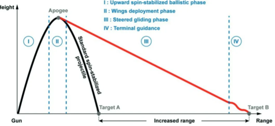
laws (guidance or terminal guidance controllers), and telemetry applications (e.g. antennas orientation to minimize data loss). It is often required in late parts of the flight where trajectory correction have to be made. A typical ballistic flight for smart shell is depicted in Figure 1.3.1. The steered gliding phase taking place after the apogee is a prime example where attitude information is useful.

Figure 1.3.1: Typical ballistic flight phases for smart artillery shells. (ISL)

1.4 Outline of the proposed solution

As explained earlier, classic attitude estimation methods can not work as-is onboard a smart shell. We will not use any rate gyro, but when needed, an estimate of the angular velocity will be developed (this estimation will be referred to as a « virtual gyro »). The 3-axis Magnetometer will be used as a body-frame measurement of the Earth magnetic field, whose coordinates b0

in the local frame are known Besides, an additional input will compensate for the missing direction measurement usually given by the 3-axis Accelerometer. The attitude will be represented under the form of a rotation matrix ˆR. A

pictorial view of the estimation method is given in Figure 1.4.1.

The « virtual gyro » can be a simple estimation of the dominant roll rate, which will be shown to be easily determined using the large oscillations observed in both transverse accelerometers and transverse magnetometers signals5.

estimate the true acceleration of the center of mass of the shell, following the classic navigation principles, see e.g. [31].

5

alternatively, one could use the knowledge of the aerodynamic moments, and the fact that 3-axis Accelerometer provides a good estimation of the angular velocities through that modeling. Of course, using aerodynamic coeﬃcients accordingly requires the knowledge

(23)

Attitude filtering

3-axis Magnetometer, b0 _ˆ

R

(virtual gyro)

Additional input

Figure 1.4.1: Attitude Filtering proposed in the thesis.

The norm of the velocity w.r.t. the air can be obtained through a fre-quency analysis of the pitching and yawing motion induced by the aerody-namic moments. This estimation uses one of the transverse accelerometer as pictured in Figure 1.4.2. It will be detailed in Chapter 3.

Velocity observer vˆ 1-axis transverse accelerometer

Figure 1.4.2: Velocity Estimation.

To compensate for the missing direction, one attitude angle will be di-rectly estimated. As will be explained, measuring only one direction makes one able to compute the attitude, up to a rotation by an unknown angle around the single known direction. If an additional « well-chosen » attitude angle is available, then the attitude estimation has only two isolated solu-tion, that can be discriminated easily. The angle under consideration is the pitch angle. It is obtained from the estimate of the velocity w.r.t. the air, as pictured in Figure 1.4.3, which gives an approximation of it under the form of the slope angle. The estimation method will be exposed in Chapter 4. The pitch angle serves as « additional input » for the attitude observer of Figure 1.4.1 as pictured in Figure 1.4.4. This will be treated in Chapter 5.

Slope angle observer ˆ

v θˆ

Figure 1.4.3: Slope angle Estimation.

Finally, by connecting all the estimates described above, one obtains the overall attitude estimation methodology proposed in the thesis. It is of the velocity.

(24)

Attitude observer ˆ

θ≈ ˆΘ Rˆ

(Virtual gyro)

Figure 1.4.4: Attitude Estimation.

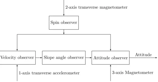
described in Figure 1.4.5. It uses a 3-axis Accelerometer (actually, only one of its transverse sensors) and a 3-axis Magnetometer. Experimental results obtained with this method will be given in Chapter 6.

Velocity observer Slope angle observer Attitude observer Spin observer

2-axis transverse magnetometer

1-axis transverse accelerometer 3-axis Magnetometer Attitude

Figure 1.4.5: Attitude Estimation Algorithm from on-board sensors.

1.5 Organization of the thesis

The manuscript is organized as follows.

Chapter 2 presents the mathematical notations employed to describe the flight dynamics of the shell under the form of a 6-degrees of freedom model of a rigid body subjected to aerodynamic forces and moments, and gravity. The two types of rotationally symmetric shells (155 mm and Basic Finner) under consideration in the thesis are described. The main equation governing the pitching and yawing motion of the shell is presented. The combined oscillations define an epicyclic motion. The set of strapdown sensors is described. Some data obtained during experimental tests serve to illustrate typical measurements observed in-flight.

(25)

In Chapter 3, the signals generated by the epicyclic motion of the shell are processed by frequency detection techniques. The frequency is related to the norm of the velocity w.r.t. the air of the shell. This relation is a key ingredient for the velocity estimator that is developed to account for observability issues near Mach 1.0.

In Chapter 4, the previously developed velocity estimation serves to es-tablish an estimation of the pitch angle of the shell. A simple linear time varying (LTV) formulation serves to establish the convergence of a Luen-berger observer, which can be replaced for sake of improved performance with an extended Kalman filter.

Chapter 5 develops an extension of the attitude complementary filter dealing with a single vector measurement and the knowledge of one angle. The convergence analysis is established.

Finally, Chapter 6 is devoted to the application of all the methods pre-sented above to real flight data, using solely on-board measurements. Com-parisons with high-fidelity measurements from a ground based position radar are provided.

(26)

Chapitre 2 - Résumé

Ce second chapitre permet la mise en équation du problème, en introduisant les différents repères utilisés, la nomenclature des différents états considérés, et les paramètres physiques propres à la munition et à son environnement. On y décrira en partie la dynamique de vol d’une munition, en distinguant dynamiques de translation et de rotation, et en mettant en évidence les équations sur lesquelles reposeront nos différentes estimations. Les différents capteurs à notre disposition sont présentés ici, ainsi que les problèmes pra-tiques auxquels leur utilisation nous confronte (accélérations d’entraînement, induction), et la structure du signal qu’ils mesurent. Bien qu’on se passe de gyromètres, on présentera également des méthodes d’estimation de vitesse angulaire simplifiée à partir des capteurs dont on dispose. Enfin, ce chapitre se conclut par la présentation du dispositif expérimental utilisé et des jeux de données considérés dans cette thèse.

(27)

(28)

Chapter 2

Mathematical formulation,

notations, flight dynamics

and instrumentation

2.1 Reference frames and Six-Degrees-of-Freedom

description

Let the frame L be defined by orthogonal unit vectors 1L, 2L, 3L where 1L direction is the direction of the shot on the horizontal plane and 3Lis vertical and pointing to the ground. This direct frame, referred to from now on as the « local frame », is an adaptation of the classical « North-East-Down » (NED) frame commonly used in aeronautics, rotated so that its first vector is oriented in the initial direction of the shot.

Classically, the shell can be modeled as a Six-Degrees-of-Freedom (6-DOF) rigid body. The full notations are summarized in Table 2.1.1. The orientation of the rigid body is defined by a set of three Tait-Bryan angles (here « ZYX » angles are chosen, following the nomenclature of [58], where, as commonly considered, the spin is defined as the rotation about its axis of least inertia). As a result, the orientation of the body with respect to the local inertial frame is described by the Tait-Bryan angle sequence:

yaw: Ψ, pitch: Θ, roll: Φ

The shell state comprises 12 variables, namely the position, velocity, attitude (under the form of the three angles previously introduced) and angular velocity. It reads

(2.1.1) Xf ull =

(

x y z vx vy vz Ψ Θ Φ p q r

(29)

x, y, z Position of the shell in the local frame

vx, vy, vz Velocity of the shell w.r.t. the local frame

h =−z > 0 Altitude of the shell

V Velocity of the shell w.r.t. the airflow

v =|V | Scalar velocity of the shell w.r.t. the airflow

Nmach Mach number of the shell

vL_B Velocity of the shell w.r.t. the local frame

X Position of the shell w.r.t. the local frame

R = [T ]LB Attitude matrix of the shell

(transition matrix from the local frame to the body frame) Ψ, Θ, Φ Tait-Bryan angles

Ψ Yaw angle

Θ Pitch angle

Φ Roll angle

Ω = (p, q, r) Angular velocity of the shell w.r.t. the local frame expressed in the body frame

ωI_L Angular velocity of the local frame w.r.t.

a geocentric frame (Earth’s rotation, adding Coriolis eﬀect)

p =⟨Ω, 1B⟩ Spin rate of the shell (or longitudinal component of Ω)

q =⟨Ω, 2B⟩ transverse component of Ω along 2B

r =⟨Ω, 3B⟩ transverse component of Ω along 3B [T ]BW Transition matrix from the body

frame to the wind velocity frame

α, β Incidence angles (see below)

α Attack angle

β Sideslip angle

αt Total angle of attack of the shell

(angle between vectors 1B and V )

θ Slope angle

(« pitch » angle of [T ]LW _{in « ZYX » decomposition)}

Table 2.1.1: Nomenclature.

This vector contains several groups of variables of interest. Let us define the following partial state variables : the position X, the velocity V (and

(30)

its norm v = |V |), three angles defining the attitude matrix R (and the corresponding quaternion q) and the angular velocity ω. Details are given in (2.1.2).

We note (e1, e2, e3) a canonical base ofR3, Ra,v the matrix defining the

3D-rotation of angle a about the vector v, and qa,v one of the two unit

quaternions representing Ra,v (see Section 5.1 for more details). Conversely,

the Ra,v matrix can be derived from the quaternion qa,v, see Section 5.1.

(2.1.2)                                X = ( x y z )T V = ( vx vy vz )T

R = [T ]LB = RΨ,e3RΘ,e2RΦ,e1

q = qΨ,e3 ⊗ qΘ,e2⊗ qΦ,e1 Ω =

(

p q r

)T

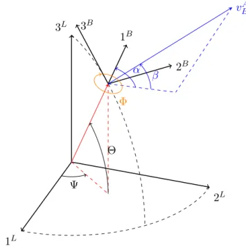
Besides the local (inertial) frame L and the body B frame, a third frame is considered and referred to as the « wind velocity frame », denoted W . It is defined from the body frame using the velocity of the shell with respect to the airflow, denoted vA_B or V , as described by Figure 2.1.1.

The attack angle α and the sideslip angle β are defined by (2.1.3) [T ]BW = R_−α,e2Rβ,e3

where [T ]BW is the transition matrix from the body frame to the wind velocity frame

The angles between the frames L, B and W are illustrated in Figure 2.1.1 (with the introduction of an intermediate frame L′) and Figure 2.1.2.

2.2 Environment model

The environment of the shell is modeled with standard atmosphere, grav-ity, and Earth magnetic field reference models. In details, following the Standardization Agreement STANAG 4355 from NATO, the gravitational acceleration at altitude h is (2.2.1) g(h) = g0 ( R R + h )2 where g0 = 9.80665× (1 − 0.0026 cos (2 Lat))

(31)

1L 2L 1L′ 2L′ Ψ 3L 1L ′ 3L 1B 3L′ Θ 2L′ 2 L′ 3L′ 2B 3B Φ 1B 1B 3B 1B′ 3W α 2B 1B ′ 2B 1W 2W β 3W

Figure 2.1.1: Definition of Tait-Bryan and incidence angles.

1L 2L 3L Ψ Θ 3B 2B 1B vA B β α Φ

Figure 2.1.2: Definition of Tait-Bryan and incidence angles at Φ = 0 ; α refers to a rotation around 2B and β around 3W.

(32)

while R is an average value of the Earth radius and Lat is the geodetic latitude of the local frame L (g slightly increases when moving away from the equator).

At any altitude h, the air density is given, following [39],

(2.2.2) ρ(h) = ρ0

(

T0− 0.0065h T0

)4.2561

with ρ0the air density on the ground. In turn, this defines the sound velocity

(2.2.3) vsound(h) = a0 ( T0− 0.0065h T0 )1 2

where a0 is the velocity of the sound at ground level. The Mach number is,

as usual,

(2.2.4) Nmach(v, h)≜

v

vsound(h)

This variable is a main input of the aerodynamic forces and moment look-up tables introduced in Section 2.3.

The various constants appearing in the previous equations are given in Table 2.2.1.

Constant value unit

ρ0 1.225 kg.m−3

a0 340.429 m.s−1

R 6.356766× 106 m

Lat 45 deg

T0 288.16 K

Table 2.2.1: Environment constants.

Throughout the thesis (in simulation and for the analysis of actual flight data), the values for the environment constants are those reported in Ta-ble 2.2.1.

2.3 Projectile model: dimensional parameters and

aerodynamic coeﬃcients

In the thesis, we consider two types of projectiles : 155 mm shells, fired with a high spin rate thanks to a rifled barrel (granting gyroscopic stability), and

(33)

Basic Finners, which are smaller and lighter, fired without any initial spin rate but possessing roll-inducing fins1.

The 155 mm is an all-purpose standard for NATO armies. The Basic Finner is a more recent experimental shell which has served for many years as a reference projectile and was tested extensively in numerous aero-ballistic ranges and in wind tunnels. The model consists of a 20 deg nose cone on a cylindrical body with four rectangular fins. The main dimensional parame-ters of the projectiles are listed in Table 2.3.1 with typical values detailed in Table 2.3.2. Reliable look-up table for their aerodynamic coeﬃcients have been established (see e.g. [102, 15, 28, 1]).

D Caliber of the shell

S Reference area of the shell

M Mass of the shell

Il Longitudinal moment of inertia

It Transverse moment of inertia

δf in cant Angle of the fins with the shell outer surface

(for Basic Finner only)

Table 2.3.1: Dimensional parameters.

Type D (m) S (m2) M (kg) Il (kg.m2) It (kg.m2)

Basic Finner 0.028 6.16× 10−4 0.4 4.36× 10−5 2.14× 10−3

155 mm 0.155 1.89× 10−2 43.25 0.15 1.61

Table 2.3.2: Type of projectiles studied.

The coeﬃcients defining the aerodynamics forces and moment are listed in Table 2.3.3. Their values are reported as a function of the Mach number in Figure 2.3.1 for the 155 mm artillery shell and in Figure 2.3.2 for the Basic Finner, for a total angle of attack of zero degree. All the variables in Table 2.3.3 are functions of (Nmach, αt).

2.4 Flight dynamics

For generality, the high velocity shell under consideration is a 6-DOF rigid body which is given both initial translational velocity and spin rate2 by

1

more precisely, a specific spin rate can be achieved by setting the initial velocity of the projectile and the angle δf in cant of its fins.

2

(34)

CD Drag force coeﬃcient

CLα Lift force coeﬃcient

Cmag−f Magnus force coeﬃcient

Cmag−m Magnus moment coeﬃcient

Clδ Rolling moment coeﬃcient

Cspin Roll damping moment coeﬃcient

CM q Pitch damping moment coeﬃcient

CM α Overturning moment coeﬃcient

Table 2.3.3: Aerodynamics coeﬃcients. All the variables in Table 2.3.3 are functions of (Nmach, αt). 0 1 2 3 Mach number CD> 0 0 1 2 3 Mach number CL,> 0 0 1 2 3 Mach number Cmag!f < 0 0 1 2 3 Mach number Cmag!m 0 1 2 3 Mach number Cl/= 0 0 1 2 3 Mach number Cspin< 0 0 1 2 3 Mach number CMq< 0 0 1 2 3 Mach number CM,> 0

Figure 2.3.1: Aerodynamic coeﬃcients profiles for 155 mm artillery shell.

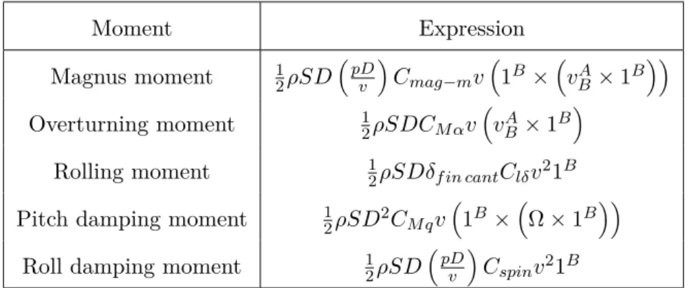
the gun launch. By contrast with rocket-propelled devices, the shell has a constant mass during the whole flight. It is subjected to drag and lift forces, Magnus forces, Coriolis force, gravity, and several moments: Magnus, overturning 3, rolling 4, pitch damping and roll damping moments [72, 60]. 3_{aerodynamic moment associated with the lift which is applied at the center of pressure.} 4

(35)

0 5 Mach number CD> 0 0 5 Mach number CL,> 0 0 5 Mach number Cmag!f = 0 0 5 Mach number Cmag!m= 0 0 5 Mach number Cl/> 0 0 5 Mach number Cspin= 0 0 5 Mach number CMq> 0 0 5 Mach number CM,> 0

Figure 2.3.2: Aerodynamic coeﬃcients profiles for Basic Finner.

These forces and moments have been extensively studied and measured using wind tunnels, free-flight ballistic ranges, spark and Schlieren photography among others methods. Experimentally established look-up tables are avail-able for the two projectiles under consideration (see e.g. [102, 15]). Concise expressions are given in Table 2.4.1 and Table 2.4.2, respectively.

Force Expression Drag force −1₂ρSCDvvAB Lift force 1₂ρSCLα ( vA_B× ( 1B× vA_B )) Magnus force 1₂ρS ( pD V ) Cmag−fv ( vA_B× 1B ) Coriolis force 2M v_BL× ω_LI Weight M g

(36)

Moment Expression Magnus moment 1₂ρSD(pD_v )Cmag−mv

( 1B_×(_vA B× 1B )) Overturning moment 1₂ρSDCM αv ( vA_B× 1B )

Rolling moment 1₂ρSDδf in cantClδv21B

Pitch damping moment 1₂ρSD2CM qv

(

1B×

(

Ω× 1B

))

Roll damping moment 1₂ρSD

(

pD v

)

Cspinv21B

Table 2.4.2: Moments applied on the shell.

2.4.1 Translational dynamics

After some reordering, the application of Newton Second Law yields, in a concise form (2.4.1) ˙v =−ρS ˜CDv 2 2M − g sin θ, ˙h = v sin θ with (2.4.2) C˜D(h, v, αt)≜ CD(Nmach(h, v), αt)

Equation (2.4.1) is obtained with some approximations, namely neglect-ing the diﬀerence between V the velocity of the shell w.r.t. the airflow and

˙

X the velocity in the local frame, and the contribution of the Coriolis force.

Those approximations are detailed in Appendix A.3.

In (2.4.1), the drag is a dominant effect and deserves some more com-ments. Some effects of the shell shape on the drag coefficient at various Mach numbers have long been studied. Those effects depend on a number of dimensionless variables. The fluid mechanism that transmits the drag force to the shell consists of two parts: surface pressure and surface shear stress (a.k.a. skin friction drag). The force generated on the forebody and the base of the shell are different. Therefore, the various components of the drag force behave in significantly different ways in the various speed regions. At subsonic flight speeds (below Mach 1.0), the drag coefficient is essentially constant. It rises sharply near Mach 1.0, then slowly decrease at higher supersonic speeds. The sudden rise appearing just below Mach 1.0 is caused by the formation of shock waves in the flow-field surrounding the shell [72]. This rise is visible in the CD profiles of Figure 2.3.1 and Figure 2.3.2.

(37)

2.4.2 Rotational dynamics

Euler equation of rotation of a rigid body subjected to external aerodynamic moments can be written under the following form. One shall note the can-cellation of the bilinear term q r in (2.4.3) due to the symmetric nature of the shell. ˙ p =ρ(h)SD 2_C spinv 2Il p +1 2ρ(h)SDδf in cantClδv 2 (2.4.3) ˙ q = 1 It ( (Il− It)p r + 1 2ρSpD 2_C mag−mvβ + 1 2ρSDCM αv 2_{α +}1 2ρSD 2_C M qvq ) (2.4.4) ˙r = 1 It ( (Il− It)p q + 1 2ρSpD 2_C mag−mvα− 1 2ρSDCM αv 2_{β +} 1 2ρSD 2_C M qvr ) (2.4.5)

As is exposed in the early work of [42], the complex reaction of the shell to aerodynamic forces and moment has a much simplified form when its axis of symmetry, its axis of rotation and the direction of motion of its center of mass though the air all coincide. This is precisely the case for the shells studied in the thesis. Actually, more advanced calculus, and several steps of careful first-order approximations5, see [72, Chapter 10], allow one to derive the equation governing the Pitching and Yawing motion of the rotationally symmetric projectiles.

Our choice of incidence angles α, β diﬀer from [72]. Ours are attached to the body, which makes it easier to relate them to the measurement of both strapdown transverse accelerometers (these angles are oscillating at the spin rate frequency), whereas in [72] the angles correspond to the horizontal and vertical oscillating motion as could be observed from the ground. Note α2

and β2, the angles considered by [72] (see Appendix A.2 for alternate angles

definition and approximation). The correspondence is given, under a small total angle of attack assumption (see Appendix A.2) by

(2.4.6)

{

α2 = sin (pt) α− cos (pt) β β2 =− cos (pt) α − sin (pt) β

By introducing the complex yaw

ξ = α2+ iβ2

5

during the whole flight (typically lasting less than 45 s for ballistic flight and less than 2 s for flat-fire) the spin rate remains very high, and the angles of attitude w.r.t. the wind frame remain small. Therefore, it is possible to study the attitude dynamics, and, in turn, the translational dynamics, under the assumption of small-angles.

(38)

one obtains the following complex valued ordinary diﬀerential equation (2.4.7) ξ +¨ v D(H− iP ) ˙ξ − v2 D2(M + iP T )ξ =−iP G with H = C_Lα∗ − C_D∗ − M D 2 It (C_{M q}∗ + C_{M α}∗ ), P = Il It pD v M = M D 2 It C_{M α}∗ , T = C_Lα∗ +M D 2 Il C_mag∗ _−m, G = gD cos Φ v2

where for each aerodynamic coeﬃcient CX one uses the scaled proxy

C_X∗ = ρSD 2M CX

The complex equation (2.4.7) will be central in the works presented in the thesis. It has been established by several authors, under various forms, which are all equivalent: [52, 53, 76, 39], among others. Also, it has been shown to be a very good approximation to the actual flight of symmetric projectiles.

This equation is a linear, second order differential equation with « almost constant » (slowly-varying) complex coefficients. Assuming now that the coefficients are indeed constants (as a short-term approximation), solving (2.4.7) reveals that the pitching and yawing motion of a symmetric projectile consists of two modes that rotate at different frequencies so that the complex yaw ξ follows an epicyclic motion in the complex plane, i.e. a motion of the general form6

ξ(t) = Aneiωnt+ Apeiωpt+ A0

(2.4.8)

where ωn and ωp << ωn designate the so-called « nutation » and «

preces-sion » angular frequencies, respectively. The epicyclic motion is pictured in Figure 2.4.1.

Going back to the « body-attached » incidence angles α and β which are, by solving (2.4.6),

(2.4.9)

{

α = sin (pt) α2− cos (pt) β2 β =− cos (pt) α2− sin (pt) β2

one has that (2.4.8) yields (2.4.10) through α + iβ =−eipt(β2+ iα2) α + iβ =−i

(

Anei(p−ωn)t+ Apei(p−ωp)t+ A0eipt

)

(2.4.10)

6

(39)

-1 1 -0.5 0 0.5 60 [deg] 0.5 [deg] 1 0 40 [s] 1.5 -0.5 20 -1 0

Figure 2.4.1: Epicyclic motion of the shell during a typical flight ; locus of the complex yaw ξ from Equation (2.4.8) [simulation results].

2.5 Onboard Sensors

2.5.1 Description of the embedded system

Figure 2.5.1: Embedded Instrumentation in a Basic Finner, from [19]. 1 Power supply unit, 2 3-axis Magnetometer, 3 3-axis Accelerometer, 4 CPU (for signal conditioning), 5 RF Transmitter, 6 Monopole Antenna.

The strapdown sensors embedded into the shells (see Figure 2.5.1) con-sists of a 3-axis Accelerometer and a 3-axis Magnetometer. The data from the sensors is collected and sent by the radio Frequency transmitter using

(40)

the cone of the shell as a monopole Antenna during the flight. The band-width allows to stream 2 megabytes of data per second with a low level of data losses7. All sensors are synchronous and sampled at the same rate (T = 124 µs for experiments, T = 100 µs in simulations).

The measurement equation are given in (2.5.1).

(2.5.1)

{

Yacc= ˙V − RTg = Fext_M − RTg = Faero_M

Ymag = RTb0

The 3-axis Accelerometer measures the proper acceleration (or acceleration relative to a free-fall) of the shell, i.e. the sum of the aerodynamic forces

Fext applied onto the shell (divided by the mass), which varies according to

1. the shell velocity (and the associated incidence)

2. its altitude (directly through the corresponding air density, and indi-rectly though the Mach number)

3. and its spin rate, mostly through Magnus eﬀect.

In turn, the 3-axis Magnetometer provides a measurement of the Earth mag-netic field b0 expressed in the body frame. Any rotation about the Earth

magnetic field vector leaves the measurement unchanged, which clearly indi-cates that the magnetometry measurements are not suﬃcient for estimating the shell attitude.

Classically, in aircraft applications where during most of the flight the applied forces compensate each other8, the actual acceleration ˙V remains

close to zero, so that the proper acceleration measured by accelerometers verifies Yacc ≃ −RTg. This is the main reason why accelerometers are

commonly used as a vector measurement, by improperly considering that they measure the vector gravity g. Under such circumstances, (2.5.1) boil down to the measurement of two linearly independent vectors (b0 being

almost never co-linear to g9), which readily allows one to solve Wahba’s problem of attitude determination.

However, in our case of free-flight, ˙V remains non-negligible from gunshot

until the end of the flight. The shell has no thrust, and is not designed in a way such that aerodynamic forces could (even approximately) compensate its weight, the two variables remaining unrelated. The proper acceleration is diﬀerent from −RTg, and the diﬀerence is strongly varying along the

7_{as will be visible when treating data, some outliers appears, especially at the end of}

the flight when the shell is the farthest from the receiving antenna.

8

mostly thanks to thrust and a design making lift suﬃcient to compensate gravity at the velocities reached thanks to the thrust.

9

(41)

trajectory, since it corresponds to the aerodynamic forces changing rapidly with the Mach number, the total angle of attack, and the altitude. This prevents us from using accelerometers as a vector measurement. We will see in the following chapters how to circumvent this problem and find a novel usage of its measurement, providing insights into incidence angles and velocities, with the help of reliable aerodynamic models.

2.5.2 Detrimental eﬀects and mitigation means Eddy currents

Once embedded into the shell, the 3-axis Magnetometer no longer directly provides a valuable vector measurement, because it is corrupted by an induc-tion effect created by the high spin rate of the electrically conductive shell. This rotation around its main axis is the root cause for eddy currents. The effects of eddy currents are mitigated by suppressing the known induction response to a given spin rate, previously modeled and measured on a testbed (see Figure 2.5.2) [19]. In the rest of the thesis, it is assumed that the induc-tion effects are already compensated for. This assumes that the spin rate is measured, which will be a question treated first of all, in Section 2.6.

Figure 2.5.2: Compensation of eddy currents eﬀect on 3-axis Magnetometer. Two blinking LEDs are synchronized for various spin rates, showing the accuracy of the model-based compensation[19].

(42)

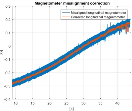
Misalignment

Ideally, the sensors should to be perfectly aligned with the body frame. In practice, there exists a (usually small) rotation between the sensors frame and the body frame, which results in a malicious modulation visible in the signals. In theory, there should be no oscillations at the spin rate frequency on the longitudinal magnetometer. This fact suggests a procedure to reduce the misalignment issue. Conversely, by applying to the 3-axis Magnetometer measurement the rotation minimizing the variance of the longitudinal com-ponent enables us to have an a posteriori better feedback. Ideally, a similar procedure could be done on the ground prior to the shot with suﬃciently fast varying external magnetic field (generated by Helmholtz bobbins). The ben-efits of the misalignment compensation, and the reduction of the variance of the signal after the rotation, is shown on real flight data in Figure 2.5.3.

10 15 20 25 30 35 40 [s] -0.4 -0.3 -0.2 -0.1 0 0.1 0.2 0.3 [G]

Magnetometer misalignment correction

Misaligned longitudinal magnetometer Corrected longitudinal magnetometer

Figure 2.5.3: Compensation of the longitudinal magnetometer misalignment. A rotation of approximately 4 deg was employed. [155 mm experimental data].

After correction of the misalignment and eddy currents, the 3-axis Mag-netometer gives signals that are close to theory, but significantly corrupted by the spin rate, as can be seen in Figure 2.5.4

(43)

4 6 8 10 12 [s] -0.35 -0.3 -0.25 -0.2 [G] 4 6 8 10 12 [s] -0.35 -0.3 -0.25 -0.2 [G] 4 6 8 10 12 [s] -0.4 -0.2 0 0.2 0.4 [G] 4 6 8 10 12 [s] -0.5 0 0.5 [G]

Figure 2.5.4: Values of longitudinal and transverse 3-axis Magnetometer sig-nals in 155 mm shell : simulation (left), experimental (right). No misalign-ment correction is shown on experimisalign-mental data, hence the heavy spin rate oscillations in the longitudinal measurement.

Fictitious forces

The accelerometers are disturbed by fictitious forces. Indeed, due to the high values of spin rate under consideration, even small misalignments (see above) or lateral shift of the sensors from the shell main axis induce substantial fictitious forces which directly corrupt the readings of the 3-axis Accelerom-eter. Interestingly, this will prove to be harmless for the frequency-based method we develop in the thesis. For reasons we will detail in Chapter 3, the dominant fictitious forces share the same frequency content as the ideal accelerometers.

In details, let Yacc0denote the proper acceleration measured at the center

of mass of the shell, then the proper acceleration occurring at a location shifted by a vector r is

(2.5.2) Yacc= Yacc0+ Ω× (Ω × r) +

dΩ dt × r

(44)

Figure 2.5.5: Instrumentation of an experimental 155 mm artillery shell from ISL. Sensors are located in the nose, thus being typically 20 cm away from the center of mass of the shell.

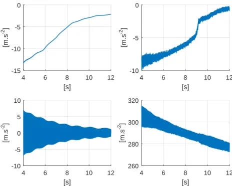
large (typically, the sensors are located approx. 20 cm from the center of mass in the direction of the nose). Furthermore, the sensors are not located right onto the shell symmetry axis, which correspond to small but non neg-ligible transverse components in r. This is due to mechanical tolerances and uncertainties in the exact location of the sensors in the shell payload case. In turn, the high spin rate has a tremendous effect even for small such transverse shift in (2.5.2). This effect is clearly visible in Figure 2.5.6 in the case of a 155 mm shell. The shift in sensors location is larger than in the case of a Basic Finner, due to the extended length of the shell. The effect is mainly due to the high values of the spin rate, and is thus negligible on low spin rate projectiles such as Basic Finner. In the case of a Basic Finner, experimental measurements are similar to the simulation feedback, even though the location of the sensors is still shifted from the center of mass of the shell.

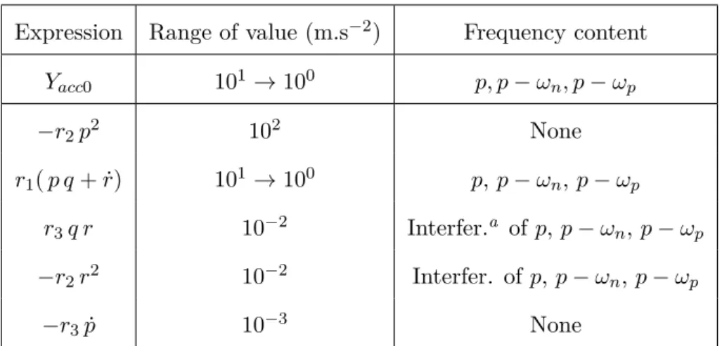
The analysis in the case of the 155 mm shell can be pursued as follows. According to (2.5.2), the factors that can cause fictitious forces are listed in Table 2.5.1, along with their typical values. In turn, the various disturbance terms appearing in (2.5.2) are listed by descending order of magnitude in Table 2.5.2. It is worth mentioning that the term r1p q + r1 ˙r is actually

much smaller than its constituting factors because, as can be seen in the last part of the rotational dynamics (2.4.5), one has that

It>> Il implies that ˙r≈ −p q

(45)

Then, it appears that the dominant fictitious force is−r2p2 and that it acts

as a (slowly drifting) bias on the 3-axis Accelerometer. The « frequency content » column in Table 2.5.2 describes the oscillating contribution of each term (q and r obeying (2.4.4) and (2.4.5), respectively, and p being almost linearly damped according to (2.4.3)). This drifting bias is visible in Figure 2.5.6 (compare bottom-left and -right plots). Interestingly the bias is very large but it does not alter the frequency content of the 3-axis Accelerometer signals. This point will be instrumental in Chapter 3.

4 6 8 10 12 [s] -15 -10 -5 0 [m.s -2 ] 4 6 8 10 12 [s] -10 -5 0 [m.s -2 ] 4 6 8 10 12 [s] -10 -5 0 5 10 [m.s -2 ] 4 6 8 10 12 [s] 260 280 300 320 [m.s -2 ]

Figure 2.5.6: Values of longitudinal and transverse 3-axis Accelerometer sig-nals: simulation (left), experimental (right).

Long. shift r1 (m) Trans. shift r2, r3 (m) p (rad.s−1) q, r (rad.s−1)

10−1 10−4 103 101

Table 2.5.1: Root causes of fictitious forces in 155 mm gyrostabilized projec-tiles.

(46)

Expression Range of value (m.s−2) Frequency content Yacc0 101→ 100 p, p− ωn, p− ωp −r2p2 102 None r1( p q + ˙r) 101→ 100 p, p− ωn, p− ωp r3q r 10−2 Interfer.a of p, p− ωn, p− ωp −r2r2 10−2 Interfer. of p, p− ωn, p− ωp −r3p˙ 10−3 None

Table 2.5.2: Signal at the center of mass and fictitious forces in one trans-verse accelerometer in a 155 mm gyrostabilized projectile.

a

wave interference: any a± b where a and b are picked from the given list.

2.6 Preliminary estimation of the angular velocity

around main axis

As already noted, the symmetric nature of the shell implies the cancellation of the bilinear term q r in (2.4.3) so that that the equation (2.4.3) governing p is almost independent on the other angular rates q and r.

The spin rate p thus has a practically autonomous dynamics with almost linear damping. On the other hand, the transverse components q, r of the angular rate are linked to the attack and sideslip angles and follows a damped oscillator dynamics similar to Equation (2.4.7).

The shell is equipped with a dummy gyrometer, which can not be ex-ploited for the various reasons mentioned in Chapter 1 It can be seen on Figure 2.5.5. We have explored various options to replace it. A two direc-tion measurement method (clearly out of the scope of the thesis) is detailed in [38], and this particular topic has been studied also in the literature (see e.g. [25, 63, 83, 65, 13]). For the shells considered in the thesis, a simpler approach can be used, by considering that the angular velocity (p, q, r) is actually close to (p, 0, 0).

Thankfully, such an estimation is easy, as the spin rate is the fastest fre-quency of both transverse accelerometers and transverse magnetometers. A frequency detection methods works well. Adding a physical model of its dy-namics (relying mostly on rolling moment and roll-damping moment) could be useful, but is not necessary. In short, an extended Kalman filter with a model ¨p = 0 yields satisfying results. Figure 2.6.1a shows results on

(47)

simu-lation data, while Figure 2.6.1b shows experimental results. For the latter, the first estimation features outliers related to magnetometer measurement outliers. This is readily solved with a complex argument calculation method more robust to outliers (see Appendix B.1.)

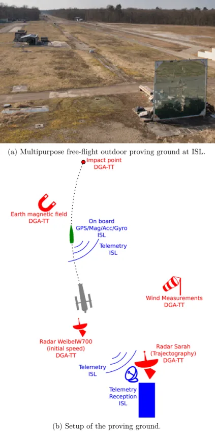
2.7 Shooting range and external instrumentation

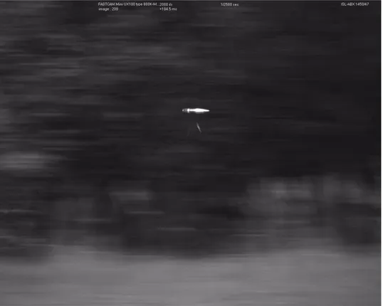
The shells are fired on the shooting range shown in Figure 2.7.1a. The setup of the shooting range is detailed in Figure 2.7.1b. This pictorial view illustrates the roles of the ground based position radar (Synthetic-aperture radar, Sarah radar) used to a posteriori reconstruct the trajectory of the shell. The ground based position radar can also be sued to reconstruct the translational velocity of the shell. The Weibel Radar is a Doppler radar used to measure the initial velocity only. The ISL telemetry system corresponds to the embedded system presented in Section 2.5 combined with ground receivers and antennas.

2.8 Testcases considered in the thesis

The four testcases listed in Table 2.8.1 will be considered in the manuscript. The reported time windows are chosen under the form of a single time in-terval avoiding instants when most data corruption issues take place. These issues are sensor saturation, data transmission losses and radar measure-ment failures. Some outliers remain in the considered data though, to keep the time windows relatively long.

(48)

Ref Pro jectile Data typ e Init. elev ation Init. v el. Max. spin Duration Time windo w angle (mil) (m.s − 1 ) rate (rad.s − 1 ) (s) (s) 1 155 mm Sim ulation 800 493 1005 56 [0 , 56] 2 155 mm Exp erimen tal 800 493 ≃ 1000 49 [8 .7 , 43] 3 Basic Finner Sim ulation 0 .2 450 0 1 [0 , 1] T able 2.8.1: Data sets considered in this thesis.

(49)

0 20 40 [s] 700 750 800 850 900 950 1000 1050 [rad.s -1 ]

Spin rate Estimation Spin rate estimation Complex argument method Spin rate reference

0 20 40 [s] -10 0 10 20 30 40 50 60 70 [rad.s -1 ]

Spin rate Estimation error

Spin rate estimation error

(a) Estimation of spin rate for a 155 mm shell [simulation results].

10 15 20 25 30 35 40 [s] 760 780 800 820 840 860 880 900 920 940 960 [rad.s -1 ]

Spin rate estimation Complex argument method

(b) Estimation of spin rate for a 155 mm shell [experimental results].

(50)

(a) Multipurpose free-flight outdoor proving ground at ISL.

(b) Setup of the proving ground.

(51)

(52)

Chapitre 3 - Résumé

Dans ce chapitre, on présente une méthode pour estimer la vitesse par rap-port à l’air d’une munition, à l’aide du contenu fréquentiel des accéléromètres, évoqué dans le chapitre précédent. Le mouvement oscillatoire de précession et de nutation de la munition est caractérisé grâce à la modélisation évoquée précédemment. On détaille ensuite les méthodes de détection de fréquence utilisées pour extraire ces diﬀérentes fréquences des signaux d’accéléromètres, puis on présente un observateur utilisant ces mesures de fréquences pour es-timer la vitesse de la munition. Une preuve de convergence est donnée, et des résultats expérimentaux sont présentés.

(53)

(54)

Chapter 3

Frequency analysis of the

epicyclic rotational dynamics

3.1 Problem statement

As will be discussed, a way to estimate the velocity w.r.t. the air of a shell submitted to known aerodynamic moments is through the analysis of the frequencies of its Pitching and Yawing oscillations. The method detailed in this chapter is instrumental for using the aerodynamic model of a gun-fired ammunition, since estimating forces requires the knowledge of its velocity with respect to the air. In our case, this is used for attitude estimation purposes as exposed in Figure 3.1.1.

As discussed in Chapter 2, the absolute values of the sensors are biased. In particular, the 3-axis Accelerometer is strongly biased by the fictitious forces. However, the bias does not impact the frequency content of the measurements. For this reason the various frequency detection methods employed in this chapter are in fact insensitive to the eﬀects of fictitious forces. Compared to other methods aiming at reconstructing the velocity w.r.t. the air, frequency detection reveals to be more reliable and accurate than more direct methods using the absolute values of the sensors such as inversion of models from accelerometric measurements.

From the description of the rotational dynamics in Section 2.4.2, the Pitching and Yawing oscillations define an epicyclic motion (depicted by Figure 2.4.1 where the locus of the complex yaw ξ from Equation (2.4.8) is shown). The frequencies of the yawing and pitching motions are visible on the measurements of the strapdown inertial sensors (although one needs to discriminate them from the spin rate oscillation beforehand, as will be explained (see Equation 2.4.7 and Table 2.5.2 for the frequency content of transverse accelerometers).

(55)

Velocity observer Slope angle observer Attitude observer Spin observer

2-axis transverse magnetometer

1-axis transverse accelerometer 3-axis Magnetometer Attitude

Figure 3.1.1: Considered cascaded estimation of the attitude. The velocity information is of interest to estimate the slope and incidence of the shell.

As it will be explained in Section 3.2, those frequencies carry information on the Mach number, the spin rate of the shell and its aerodynamics coeﬃ-cients. The methodology we advocate is pictured in Figure 3.1.2. However, the frequency information can be more or less diﬃcult to extract, especially in the trans-sonic region. For this reason, the methodology combines a fre-quency detection algorithm and a state observer playing the role of filter.

Frequency detection Velocity observer transverse accelerometer ˆ h, ˆp 6-DOF model ˆ v

Figure 3.1.2: Method to estimate the velocity of the shell.

3.2 Frequency content of the embedded inertial

measurements

Some lengthy calculations allow one to determine the frequencies appearing in the solution of the rotational dynamics (2.4.7). These frequencies are the

(56)

results of some wave interferences1 caused by the nutation, precession and spin rotations.

The nutation and precession frequencies, ωn and ωp < ωn respectively,

have symmetrical expressions (3.2.1) ωn= pIl 2It + v 2D(P 2 1 + P22) 1 4cos [ 1 2arctan ( P2 P1 )] (3.2.2) ωp= pIl 2It − v 2D(P 2 1 + P22) 1 4 cos [ 1 2arctan ( P2 P1 )] where P1(v, h, p) = a1(v, h)2− b1(v, p)2− 4a2(v, h) P2(v, h, p) = 4b2(v, h, p)− 2a1(v, h)b1(v, h) with a1(v, h) =−BMCM q+ BF(CLα− CD) a2(v, h) =−BMCM α b1(v, p) = p vD Il It b2(v, h, p) = b1(BFCLα− BMCmag−m It Il ) BF(h) = ρa(h)SD 2m , BM(h) = ρa(h)SD3 2It

3.3 Instantaneous frequency detection: measuring

varying frequencies

3.3.1 Definition of the frequency of interest

As discussed in Section 2.5, the transverse strapdown accelerometers mea-sure a projection of the aerodynamic forces in the body frame. Their signal is thus proportional to the incidence angles of the shell. Typical measure-ments are reported in Figure 3.3.1. According to (2.4.10), these angles oscillate with frequencies

{p − ωn, p− ωp, p}

where ωn and ωp are the precession and nutation frequencies (refered to as

« epicyclic frequencies ») defined in eqs. (3.2.1) and (3.2.2). 1

(recall from Chapter 2.) wave interference between a and b are any a± b ; here, only p, p− ωnand p− ωpshow in the signal due to the peculiar expression of the accelerometer

(57)

16 16.05 16.1 16.15 16.2 16.25 16.3 16.35 16.4 16.45 16.5 260 265 270 32 32.05 32.1 32.15 32.2 32.25 32.3 32.35 32.4 32.45 32.5 228 230 232 45 45.05 45.1 45.15 45.2 45.25 45.3 45.35 45.4 45.45 45.5 195 200 205

Figure 3.3.1: Examples of signals from one of the transverse accelerometers. Three distinct time windows are reported. [experimental results]. Signals with and without noise filtering are shown.

In the following, we define our « measurement » ωmeas as

(3.3.1) ωmeas = ωn− p 2 Il It = p 2 Il It − ωp = ωn− ωp 2

There are a number of possible choices to isolate the velocity-dependent factor appearing in the equations. Because p is easy to estimate as discussed in Section 2.6, a simple strategy is to simply subtract it from the detected frequencies.

Figure 3.3.2 shows the frequency content of a transverse accelerometer, and the epicyclic frequencies themselves, over the course of a typical ballistic flight. The nutation frequency ωn, faster than the precession ωp, is both

easier to measure on short time windows (because a larger number of its periods can be observed over a given time window) and to distinguish from the spin rate in the accelerometer feedback (see Figure 3.3.2-right). For these reasons, we now focus on detecting the nutation frequency ωn.