An integrated GIS-based and spatiotemporal analysis of traffic accidents: a case study in Sherbrooke

i

Université de Sherbrooke

An Integrated GIS-Based and Spatiotemporal Analysis of Traffic Accidents:

A Case Study in Sherbrooke

Homayoun Harirforoush

Thèse présentée pour l'obtention du grade de Philosophiae Doctor (Ph.D.) en télédétection

May 2017

©

Département de géographie et télédétection Faculté des lettres et sciences humaines

iii

Composition du jury

Cette thèse a été évaluée par un jury composé des personnes suivantes

Prof. Lynda Bellalite, directeure de recherche

Département de géomatique appliquée, FLSH, Université de Sherbrooke

Prof. Goze Bertin Bénié, codirecteur de recherche

Département de géomatique appliquée, FLSH, Université de Sherbrooke

Prof. Jérôme Théau, examinateur interne

Département de géomatique appliquée, FLSH, Université de Sherbrooke

Dr. Mickaël Germain, examinateur interne

Département de géomatique appliquée, FLSH, Université de Sherbrooke

Prof. Luis F. Miranda-Moreno, examinateur externe

iv

Résumé

Les accidents de la route sont responsables de plus de 1500 décès par année au Canada et ont des effets néfastes sur la société. Aux yeux des autorités en transport, il devient impératif d’en réduire les impacts. Il s’agit d’une préoccupation majeure au Québec depuis que les risques d’accidents augmentent chaque année au rythme de la population. En réalité, les accidents routiers se produisent rarement de façon aléatoire dans l’espace-temps. Ils surviennent généralement à des endroits spécifiques notamment aux intersections, dans les bretelles d’accès, sur les chantiers routiers, etc. De plus, les conditions climatiques associées aux saisons constituent l’un des facteurs environnementaux à risque affectant les taux d’accidents. Par conséquent, il devient impératif pour les ingénieurs en sécurité routière de localiser ces accidents de façon plus précise dans le temps (moment) et dans l’espace (endroit). Cependant, les accidents routiers sont influencés par d’importants facteurs comme le volume de circulation, les conditions climatiques, la géométrie de la route, etc. Le but de cette étude consiste donc à identifier les points chauds au moyen d’un historique des données d’accidents et de leurs répartitions spatiotemporelles en vue d’améliorer la sécurité routière.

Cette thèse propose deux nouvelles méthodes permettant d’identifier les points chauds à l’intérieur d’un réseau routier. La première méthode peut être utilisée afin d’identifier et de prioriser les points chauds dans les cas où les données sur le volume de circulation sont disponibles alors que la deuxième méthode est utile dans les cas où ces informations sont absentes. Ces méthodes ont été conçues en utilisant des données d’accidents sur trois ans (2011-2013) survenus à Sherbrooke. La première méthode propose une approche intégrée en deux étapes afin d’identifier les points chauds au sein du réseau routier. La première étape s’appuie sur une méthode d’analyse spatiale connue sous le nom d’estimation par noyau. La deuxième étape repose sur une méthode de balayage du réseau routier en utilisant les taux critiques d’accidents, une démarche éprouvée et

v

décrite dans le manuel de sécurité routière. Lorsque la densité des accidents routiers a été calculée au moyen de l’estimation par noyau, les points chauds potentiels sont ensuite testés à l’aide des taux critiques. La seconde méthode propose une approche intégrée destinée à analyser les distributions spatiales et temporelles des accidents et à les classer selon leur niveau de signification. La répartition des accidents selon les saisons a été analysée à l’aide de l’estimation par noyau, puis ces valeurs ont été assignées comme attributs dans le test de signification de Moran.

Les résultats de la première méthode démontrent que plus de 90 % des points chauds à Sherbrooke sont concentrés aux intersections et au centre-ville où les conflits entre les usagers de la route sont élevés. Ils révèlent aussi que les intersections contrôlées sont plus à risque par comparaison aux intersections non contrôlées et que plus de la moitié des points chauds (58 %) sont situés aux intersections à quatre branches (en croix). Les résultats de la deuxième méthode montrent que les distributions d’accidents varient selon les saisons et à certains moments de l’année. Les répartitions saisonnières montrent des tendances à la densification durant l’été, l’automne et l’hiver alors que les distributions sont plus dispersées au cours du printemps. Nos observations indiquent aussi que les répartitions ayant considéré la sévérité des accidents sont plus denses que les résultats ayant recours au simple cumul des accidents.

Les résultats démontrent clairement que les méthodes proposées peuvent: premièrement, aider les autorités en transport en identifiant rapidement les sites les plus à risque à l’intérieur du réseau routier; deuxièmement, prioriser les points chauds en ordre décroissant plus efficacement et de manière significative; troisièmement, estimer l’interrelation entre les accidents routiers et les saisons.

Mots clés: Accidents routiers, point chaud, taux d’accidents, système d’information géographique,

vi

Abstract

Road traffic accidents claim more than 1,500 lives each year in Canada and affect society adversely, so transport authorities must reduce their impact. This is a major concern in Quebec, where the traffic-accident risks increase year by year proportionally to provincial population growth. In reality, the occurrence of traffic crashes is rarely random in space-time; they tend to cluster in specific areas such as intersections, ramps, and work zones. Moreover, weather stands out as an environmental risk factor that affects the crash rate. Therefore, traffic-safety engineers need to accurately identify the location and time of traffic accidents. The occurrence of such accidents actually is determined by some important factors, including traffic volume, weather conditions, and geometric design. This study aimed at identifying hotspot locations based on a historical crash data set and spatiotemporal patterns of traffic accidents with a view to improving road safety.

This thesis proposes two new methods for identifying hotspot locations on a road network. The first method could be used to identify and rank hotspot locations in cases in which the value of traffic volume is available, while the second method is useful in cases in which the value of traffic volume is not. These methods were examined with three years of traffic-accident data (2011–2013) in Sherbrooke. The first method proposes a two-step integrated approach for identifying traffic-accident hotspots on a road network. The first step included a spatial-analysis method called network kernel-density estimation. The second step involved a network-screening method using the critical crash rate, which is described in the Highway Safety Manual. Once the traffic-accident density had been estimated using the network kernel-density estimation method, the selected potential hotspot locations were then tested with the critical-crash-rate method. The second method offers an integrated approach to analyzing spatial and temporal (spatiotemporal) patterns of traffic accidents and organizes them according to their level of significance. The spatiotemporal seasonal

vii

patterns of traffic accidents were analyzed using the kernel-density estimation; it was then applied as the attribute for a significance test using the local Moran’s I index value.

The results of the first method demonstrated that over 90% of hotspot locations in Sherbrooke were located at intersections and in a downtown area with significant conflicts between road users. It also showed that signalized intersections were more dangerous than unsignalized ones; over half (58%) of the hotspot locations were located at four-leg signalized intersections. The results of the second method show that crash patterns varied according to season and during certain time periods. Total seasonal patterns revealed denser trends and patterns during the summer, fall, and winter, then a steady trend and pattern during the spring. Our findings also illustrated that crash patterns that applied accident severity were denser than the results that only involved the observed crash counts.

The results clearly show that the proposed methods could assist transport authorities in quickly identifying the most hazardous sites in a road network, prioritizing hotspot locations in a decreasing order more efficiently, and assessing the relationship between traffic accidents and seasons.

Keywords: Traffic accidents, hotspot, crash rate, geographic information system (GIS), spatial

viii

Sommaire

Les accidents de la route engendrent des coûts sociaux et économiques importants pour la société. Selon l’Organisation mondiale de la santé, les accidents routiers sont à l’origine de plus d’un million de décès de même que de vingt à cinquante millions de victimes chaque année. Les accidents routiers représentent la huitième cause de mortalité au monde et se hisseront au cinquième rang d’ici 2030 si aucune action n’est entreprise.

Au Canada, on dénombre près de 900 000 kilomètres de routes, incluant les liaisons régionales et les autoroutes nationales. En 2012, environ 1823 décès et 122 140 blessés sont survenus sur les réseaux routiers canadiens. Au Québec, on recense environ 137 000 kilomètres de route et, en 2012, près de 39 541 collisions se sont produites sur son réseau routier. Le taux de mortalité moyen était de 6,1 décès par 100 000 habitants. En 2012, près de 2529 accidents ont eu lieu à Sherbrooke sur son réseau routier. Le taux de mortalité moyen s’élève à 6,3 décès par 100 000 habitants. Les résultats montrent aussi que le taux d’accidents à Sherbrooke est plus élevé que la moyenne canadienne.

Afin de réduire le nombre de décès et d’accidents sévères de façon significative, il est nécessaire de comprendre où et quand se produisent les accidents. Une recension des études antérieures révèle que les accidents sont, en réalité, rarement aléatoires dans l’espace-temps et qu’ils sont souvent regroupés à des endroits spécifiques. La raison principale de cette occurrence dépend de plusieurs facteurs dont l’exposition au danger (mesurée généralement par le volume de circulation), les caractéristiques environnementales comme les conditions climatiques (neige, pluie, brouillard), la géométrie de la route (virage prononcé, pente abrupte) et bien d’autres.

L’analyse géospatiale de regroupements au moyen d’un système d’information géographique constitue une approche appropriée afin d’identifier la localisation d’un ou plusieurs semis de points.

ix

Le regroupement spatial correspond au processus par lequel on regroupe des objets similaires sous forme de semis de points ou de classes, basé sur leur densité, leur connectivité ou leur distance. Un agrégat d’accidents routiers localisé à un endroit correspond à une configuration où la densité d’accidents y est très élevée. La méthode d’estimation par noyau est une technique destinée à détecter l’existence de points chauds à l’intérieur d’un réseau routier.

Au fil des ans, de nombreuses méthodes d’analyse spatiale ont été proposées et appliquées afin d’identifier les agrégats d’accidents routiers (points chauds). Ces études utilisent généralement la méthode d’estimation par noyau. On pourrait croire qu’elles sont parvenues à localiser les points chauds. Cependant, ces études comportent certaines limitations et négligent des aspects importants dans l’analyse des données d’accidents. En premier lieu, certaines études ont considéré uniquement des données brutes d’accidents (accidents observés) dans leur analyse. Dans les faits, ces études n’ont pas considéré d’autres paramètres de sécurité comme l’exposition au risque, ce qui peut mener à des informations erronées sur les sites prédisposés à une intervention. À ce propos, le volume de circulation constitue l’indicateur le plus courant pour mesurer l’exposition au risque. En second lieu, les études existantes ont recours à des données agrégées sur une longue période pour chaque site sans savoir si ces accidents s’y produisent de façon récurrente. Elles ne considèrent pas le fait que les accidents peuvent être dus au hasard ou associés à un problème récurrent lié à la géométrie de la route. En général, l’occurrence des accidents à un endroit varie d’une année à l’autre, autour d’une valeur moyenne. Néanmoins, en raison des variations aléatoires des accidents routiers, les cas extrêmes survenant au cours d’une année peuvent donner lieu à des fréquences faibles l’année suivante. En troisième lieu, dans les études antérieures, les chercheurs ont eu recours exclusivement à des cumuls d’accidents (sur l’année entière) et traitent indifféremment les accidents. En fait, ils ne tiennent pas compte de la corrélation entre les saisons et les accidents, alors que la distribution des accidents fluctue d’un mois à l’autre et entre les années. À titre indicatif, les conditions climatiques constituent un facteur environnemental à risque qui affecte le

x

taux d’accidents. En quatrième lieu, la plupart des recherches existantes utilisent des données brutes d’accidents et portent une attention inadéquate aux différents niveaux de gravité des accidents. Ces études ne font aucune distinction quant à la sévérité des accidents (ex.: dommages matériels seulement, accidents avec blessés et collisions fatales) et traitent indifféremment les trois types d’accidents. Par conséquent, il s’avère nécessaire de trouver un moyen de relever la distribution des accidents et d’identifier les sites dangereux au sein d’un réseau routier.

L’objectif principal de cette recherche consiste à identifier les points chauds sur la base de l’historique de données d’accidents routiers et sur leurs distributions spatiotemporelles en vue d’améliorer la sécurité routière. Le fait de connaître la localisation des points chauds et la manière de les éviter permet de réduire le nombre de collisions en milieu urbain.

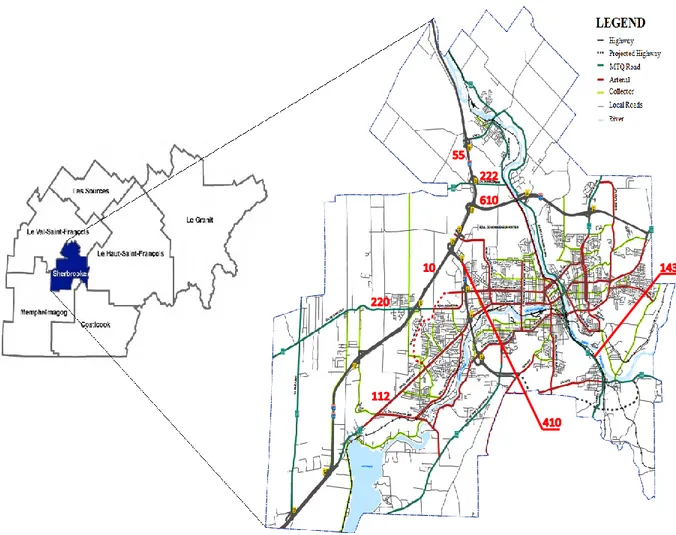
La recherche a été menée sur le territoire de la ville de Sherbrooke en raison de la disponibilité des ressources et des données quantitatives. Ces données comprennent l’information sur le réseau routier, les données d’accidents de même que le volume de circulation à partir de diverses sources auxquelles on a eu recours afin de développer l’une des méthodes proposées.

Cette thèse propose deux nouvelles méthodes (articles) afin de localiser les points chauds à l’intérieur d’un réseau routier. La première méthode peut être utilisée afin d’identifier et de prioriser les points chauds lorsque les données sur le volume de circulation sont accessibles alors que la seconde méthode est conçue dans les cas où ces informations ne sont pas disponibles.

Dans le premier article, nous proposons une approche afin de sélectionner des sites particuliers à partir des résultats issus de l’estimation par noyau en vue d’une analyse ultérieure. Ainsi, à l’encontre des autres études qui utilisent des données brutes d’accidents, nous avons eu recours aux résultats de l’estimation par noyau avec une densité supérieure à trois écarts types au-delà de la moyenne. Cette approche a permis de sélectionner non seulement les sites où la fréquence des accidents est supérieure à la norme, mais également d’identifier les sites où le problème est

xi

récurrent, pouvant être attribuable à une défaillance du réseau routier et non pas au hasard. La comparaison entre les points chauds obtenus à partir de l’intégration des données sur trois ans avec ceux des données agrégées globalement sur la même période révèle que la démarche proposée améliore la détection des points chauds.

Le premier objectif de cet article consistait à démontrer la manière dont le volume de circulation affecte la détermination des points chauds. Afin d’y parvenir, il a fallu combiner l’estimation par noyau et le taux critique d’accidents. La méthode du taux critique a été retenue dans cette étude, car elle considère le volume de circulation. La comparaison entre les résultats obtenus au moyen du volume de circulation et des données d’accidents avec ceux obtenus à partir des données d’accidents uniquement révèle que le nombre de points chauds a diminué de 128 à 20 sites (une réduction équivalant à 84 % du nombre de points chauds). Cette différence considérable entre les deux expériences est attribuable à l’effet du volume de circulation. Le nombre d’accidents routiers survenant à un endroit est fonction du risque d’exposition. Par conséquent, cette méthode permet d’écarter les sites jugés sécuritaires et de concentrer les ressources aux endroits où le problème n’est pas documenté.

Le second objectif du premier article visait à démontrer que l’identification des points chauds est plus efficace en combinant l’analyse spatiale au moyen de l’estimation par noyau et la technique du manuel de sécurité routière. L’examen des résultats démontre clairement que l’approche intégrée en deux étapes a modifié la représentation des points chauds, passant d’un simple agrégat d’accidents routiers à une distribution de sites à risque. Cette approche considère des variables significatives en matière de sécurité routière, dont le volume de circulation (exposition au risque), la nature aléatoire des accidents, le type d’intersection et la variance des accidents. Les résultats montrent de façon évidente que les accidents routiers surviennent majoritairement aux intersections (90 %) où le niveau de conflit entre les divers usagers de la route est le plus élevé. Ce phénomène pourrait être attribuable à de nombreux facteurs, dont une signalisation routière inappropriée ou

xii

une géométrie de la route déficiente. Les résultats ont aussi révélé que les intersections contrôlées (particulièrement les intersections en croix) sont plus à risque en raison des mouvements plus nombreux qui s’y produisent par comparaison aux intersections non contrôlées. De même, les intersections à trois branches (intersections en T) sont plus sécuritaires que celles en croix. Les résultats montrent qu’il est possible de prioriser les intersections en vue d’interventions destinées à réduire les accidents. Les résultats ont permis de classer les sites à risque en ordre décroissant et d’attribuer une priorité plus élevée aux sites où les différences sont plus marquées entre les taux d’accidents et le taux critique. Les résultats montrent que les sites prioritaires à Sherbrooke sont localisés majoritairement au centre-ville et à proximité d’endroits achalandés comme le Cégep de Sherbrooke et l’hôpital Fleurimont (CHUS).

Dans le second article, nous avons intégré la méthode d’estimation par noyau et l’indice de Moran afin de déterminer les regroupements significatifs. L’estimation par noyau a été retenue, car elle s’avère utile pour analyser les propriétés des accidents routiers et pour calculer la variation autour de la moyenne. Comme les tests de signification des semis de points sont inexistants, le niveau de signification a été testé à l’aide de l’indice de Moran. De façon plus précise, l’indice de Moran utilise les densités obtenues au moyen de l’estimation par noyau comme attribut afin d’évaluer le niveau de signification des sites identifiés à haute densité d’accidents. Une recension des recherches antérieures révèle que peu d’études ont combiné l’estimation par noyau à des tests statistiques. Cette étape permet de sélectionner les semis de points/anomalies (les sites à risque) et évite la multiplication des regroupements.

Le premier objectif du second article consistait à étudier l’interrelation entre les saisons et le nombre d’accidents au moyen d’une analyse spatiotemporelle. Afin d’y parvenir, cette analyse a été menée en recourant à l’estimation par noyau, combinée à des cartes d’association. Les résultats révèlent que la distribution des accidents diffère selon les saisons et à certaines périodes de l’année. La répartition des accidents survenus entre 2011 et 2013 révèle une distribution plus dense durant

xiii

l’été, l’automne et l’hiver par comparaison à une distribution plus homogène et régulière au printemps. Cela permet aux autorités et aux planificateurs en transport de se concentrer sur des endroits particuliers, à des moments précis de l’année. De plus, l’approche proposée permet d’identifier les zones à risque selon les saisons. À nouveau, la détection de ces sites permet aux autorités et aux planificateurs en transport d’allouer de manière plus efficace les sommes et les ressources nécessaires à l’amélioration de la sécurité routière.

Le deuxième objectif du second article consistait à examiner l’influence des saisons sur la gravité des accidents. Ainsi, contrairement aux recherches antérieures qui ont négligé cet aspect, l’actuelle étude examine l’influence des saisons sur la gravité des accidents et leur distribution. Nos résultats montrent clairement que les cartes d’association basées sur la gravité des accidents (représentées dans l’expérience II) ont une distribution plus dense que celles utilisant uniquement le nombre d’accidents (représentées dans l’expérience I). À titre indicatif, le nombre significatif de points chauds de l’expérience II (239 zones) est plus élevé que celui de l’expérience I (105 zones) à un seuil de signification de 0,05. Contrairement à l’expérience I où les zones denses sont localisées majoritairement au centre-ville et aux intersections importantes, dans l’expérience II, les zones denses sont davantage dispersées à travers le réseau routier. La différence entre ces deux expériences permet de mettre en lumière l’impact de la gravité des accidents, dont le nombre d’accidents avec blessés et le nombre de décès.

Cette étude repose sur un large échantillon d’accidents (6926 collisions) et sur un territoire couvrant la totalité d’un réseau routier (à l’échelle municipale). De plus, nous avons proposé et développé deux approches afin d’identifier les sites à risque en milieu urbain. La première approche plus complexe (présentée dans le premier article) peut s’appliquer dans les cas où les données sur le volume de circulation sont disponibles. La deuxième approche (présentée dans le second article) peut être utilisée dans les cas où ces informations sont absentes. Les approches proposées peuvent

xiv

fournir une aide précieuse aux autorités en transport afin d’identifier rapidement les sites dangereux à l’intérieur d’un réseau routier.

xv

Table of contents

List of Figures ... xviii

List of Tables ... xix

Acknowledgments ... xx

Glossary of Terms – Quick Reference Guide ... xxi

List of Abbreviations ... xxiii

1. Introduction ... 1 1.1 Background ... 1 1.2 Problem Statement... 3 1.3 Objective ... 6 1.4 Hypotheses ... 7 1.5 Limitations ... 7 1.6 Thesis Contributions ... 8 1.7 Thesis Structure ... 10 2. Literature Review ... 11 2.1 Spatial Modeling ... 11 2.2 Non-Spatial Modeling ... 16 2.2.1 Accident Frequency ... 17

2.2.2 Crash Rate Method ... 17

2.2.3 Critical Crash Rate Method ... 17

2.2.4 Equivalent Property Damage Only Method ... 18

2.2.5 Relative Severity Index Method ... 18

2.3 Crash Prediction Models ... 18

2.3.1 Level of Service of Safety (LOSS) ... 19

2.3.2 Excess Predicted Average Crash Frequency Using SPFs... 19

2.4 Empirical Bayes Method ... 20

2.4.1 Expected Average Crash Frequency with EB Adjustment ... 20

2.4.2 EPDO Average Crash Frequency with EB Adjustment ... 21

2.4.3 Excess Expected Average Crash Frequency with EB Adjustment ... 21

2.5 Observed Heterogeneity Counts Modeling ... 21

2.6 Unobserved Heterogeneity Counts Modeling ... 22

3. Study Data ... 25

xvi

3.2 Road-Network Base Map ... 27

3.3 Collision Data ... 28 3.4 Traffic Volume ... 28 4. First Article ... 30 4.1 Background ... 30 4.1.1 Methods ... 30 4.1.2 Discussion... 34 4.2 Introduction ... 38 4.3 Study Data ... 42 4.4 Methods ... 44 4.4.1 Network KDE ... 44 4.4.2 Threshold selection ... 48 4.4.3 Potential hotspots ... 48

4.4.4 Prediction accuracy index ... 49

4.4.5 Critical crash rate ... 50

4.5 Analysis Results ... 52

4.5.1 Results of three years of observed crash data using network KDE ... 52

4.5.2 Exploring potential hotspot locations ... 54

4.5.3 Method comparison ... 57

4.5.4 Hotspot identification using the critical crash rate ... 58

4.6 Discussion and Conclusion ... 61

5. Second Article ... 64

5.1 Background ... 64

5.2 Methods ... 64

5.3 Discussion ... 66

5.4 Introduction ... 70

5.5 Data and Methods ... 72

5.5.1 Data used in this study ... 72

5.6 Methods ... 74

5.6.1 Kernel density estimation ... 74

5.6.2 CoMap ... 75

5.6.3 Local Moran’s I ... 77

5.7 Analysis Results ... 78

xvii

5.7.2 Influence of various seasons on collision severity (Experiment II)... 81

5.8 Discussion and Conclusions ... 84

6. Discussion and Conclusion ... 87

7. Appendices ... 96

xviii

List of Figures

FIG. 3.1 THE URBAN DESIGN FRAMEWORK OF SHERBROOKE (VILLE DE SHERBROOKE,

2013) ... 25

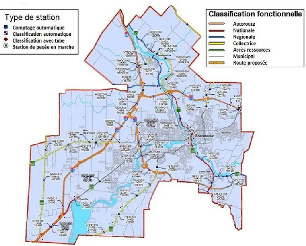
FIG. 3.2 MAP OF THE STUDY AREA (VILLE DE SHERBROOKE, 2013) ... 27 FIG. 3.3 METERING STATIONS IN SHERBROOKE (QUEBEC’S MINISTRY OF

TRANSPORTATION, 2014) ... 29

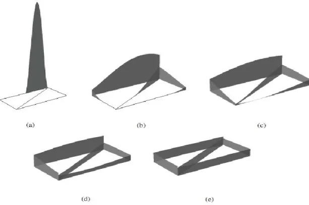
FIG. 4.1 BEHAVIOR OF THE KERNEL FUNCTION WITH VARIOUS SEARCH RADII (SUGIHARA

ET AL., 2010) ... 31

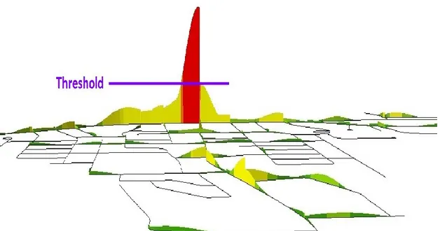
FIG. 4.2 THREE-DIMENSIONAL EXAMPLE OF A THREE-STANDARD-DEVIATION THRESHOLD

ON QUEEN STREET ... 32

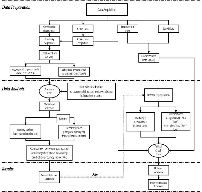
FIG. 4.3 FLOWCHART OF THE PROPOSED METHOD: (A) SELECTED METHODS FROM

DIFFERENT SAFETY ANALYSIS, AND (B) METHODOLOGY ... 34

FIG. 4.4 THE STUDY AREA (SHERBROOKE, CANADA) ... 43 FIG. 4.5 SIMPLIFIED EXAMPLE OF AN EQUAL SPLIT DISCONTINUOUS KERNEL FUNCTION

(MODIFIED FROM OKABE AND SUGIHARA, 2012) ... 45

FIG. 4.6 DIFFERENT SEARCH BANDWIDTHS (50,100, 300, AND 500 M) AND THEIR IMPACT ON

THE DENSITY SURFACE ... 47

FIG. 4.7 MERGING THREE COLLISION DENSITY MAPS (2011, 2012, AND 2013) ... 49 FIG. 4.8 NETWORK-KDE RESULTS BASED ON THREE YEARS OF AGGREGATED CRASH DATA

... 53

FIG. 4.9 COLLISION-DENSITY MAPS HIGHER THAN THE THRESHOLD FOR THREE

CONSECUTIVE YEARS: (A) 2011, (B) 2012, AND (C) 2013 ... 56

FIG. 4.10 POTENTIAL HOTSPOT LOCATIONS ... 57 FIG. 4.11 HOTSPOT LOCATIONS IN THE CITY OF SHERBROOKE ... 61 FIG. 5.1 FLOWCHART OF THE PROPOSED METHOD: (A) SELECTED METHODS FROM

DIFFERENT SAFETY ANALYSIS, AND (B) METHODOLOGY ... 66

FIG. 5.2 STUDY AREA WITH DISTRIBUTION OF ALL CRASHES IN SHERBROOKE (2011–2013)

... 74

FIG. 5.3 UNIVARIATE COMAP FOR ALL TRAFFIC ACCIDENTS IN SHERBROOKE. THE

ORANGE BARS SHOW THE SAMPLING PERIODS FOR EACH SERIES OF IMAGES (I.E., PANEL 1 FOR WINTER, PANEL 2 FOR SPRING, PANEL 3 FOR SUMMER, PANEL 4 FOR FALL) ... 79

FIG. 5.4 UNIVARIATE COMAP REPRESENTING SEASON-RELATED HOTSPOT LOCATIONS

xix

FIG. 5.5 UNIVARIATE COMAP FOR ALL CRASHES IN SHERBROOKE (BASED ON CRASH

SEVERITY). THE ORANGE BARS SHOW THE SAMPLING PERIODS FOR EACH SERIES OF IMAGES. THE BAR GRAPHS ONLY SHOW THE RELATED NUMBER OF SLIGHT-INJURY

AND FATAL- / SEVERE-INJURY CRASHES FOR EACH SAMPLING PERIOD. ... 82

FIG. 5.6 BIVARIATE COMAP TO COMPARE THE DENSITY VALUES OF SIMPLE COLLISION COUNTS (EXPERIMENT I) AND TRAFFIC ACCIDENTS BASED ON COLLISION SEVERITY (EXPERIMENT II) ... 84

FIG. 6.1 INTERPRETATION OF RESULTS EXAMPLES: (A) WANG (2012); (B) KUNDAKCI (2014); ... 94

FIG. 7.1 INCREMENTAL SPATIAL AUTOCORRELATION RESULT ... 96

List of Tables

TABLE 2.1 SELECTED PUBLICATIONS RELATED TO IDENTIFYING THE SPATIAL CLUSTERING OF TRAFFIC ACCIDENTS BY TYPE OF SPATIAL STATISTIC ... 14

TABLE 4.1 COMPARISON BETWEEN TWO NETWORK-KDE RESULTS ... 58

TABLE 4.2 TWENTY (20) HOTSPOT LOCATIONS BASED ON THE CRITICAL-CRASH-RATE METHOD. ... 59

TABLE 5.1 DIFFERENT ZONES OF LOCAL MORAN’S I ... 65

TABLE 5.2 DESCRIPTION OF TRAFFIC-ACCIDENT TYPES. ... 73

TABLE 5.3 CRASHES CLASSIFIED INTO FOUR SAMPLING PERIODS ... 76

TABLE 5.4 THE NUMBER OF SIGNIFICANT H–H AREAS FOR TWO EXPERIMENTS AT DIFFERENT SIGNIFICANCE LEVELS (P-VALUE) ... 83

xx

Acknowledgments

I would like to take this opportunity to thank all the people who helped me in completing this thesis.

First and foremost, I would like to express my extreme gratitude to my supervisor, Professor Lynda Bellalite, for her scientific guidance, advice, concern, and continuous support throughout my study. I would also like to thank my co-supervisor, Professor Goze Bertin Bénié, for his concern, suggestions, and support throughout my study. I am also grateful to them for their financial support. I thoroughly enjoyed working with them, and I learned a great deal from them, both academically and in everyday life.

I would like to thank the panel members for their time and for the honor of having agreed to examine my work. I am grateful to the Ministère des Transport (Québec) and Ville de Sherbrooke for the data provided.

Finally, I would like thank my family for their constant encouragement, support, and love. I would not have been able to complete my research and this thesis without their endless love.

xxi

Glossary of Terms – Quick Reference Guide

Cluster analysis —The task of grouping the set of objects in such a way that objects in the same group (called a cluster) are more similar to each other than to those in other groups (clusters).

Clustered distribution — Many points are concentrated close together and large areas that contain

very few points.

Crash rate — The number of crashes that occur at a given site during a certain time period in relation to a particular measure of exposure (e.g., per million vehicle miles of travel for a roadway segment).

Crash severity — The level of injury or property damage due to a crash.

Kernel-density estimation — A non-parametric way to estimate the probability density function of a random variable.

Kernel function — A weighting function used in non-parametric estimation techniques. Kernels are used in kernel-density estimation to estimate a random variable’s density function.

Point-pattern analysis — The evaluation of the pattern, or distribution, of a set of points on a surface.

Property-damage-only crash — A crash that involves a loss of all or part of the transporting vehicle, but no injuries or fatalities.

Random distribution — Any point is equally likely to occur at any location and the position of any point is not affected by the position of any other point.

Road hotspot — Represents a road location considered high risk with respect to the probability of traffic accidents in comparison to the risk level of the surrounding areas (Basically, it refers to area with an unusually high occurrence of traffic accidents).

xxii

Spatialanalysis— The process of examining the locations, attributes, and relationships of features in spatial data using overlays and other analytical techniques in order to address a question or gain useful knowledge. Spatial analysis extracts or creates new information from spatial data.

Spatial clustering — The process of grouping a set of spatial objects into meaningful subclasses (that is, clusters) so that a cluster’s members are as similar as possible, whereas the members of different clusters differ as much as possible from each other.

Spatial autocorrelation — A measure of the degree to which a set of spatial features and their associated data values tend to be clustered together in space (positive spatial autocorrelation) or dispersed (negative spatial autocorrelation).

xxiii

List of Abbreviations

Symbol

Definition

AADT Average Annual Daily Traffic Volumes

CBD Central Business District

CCS Continuous Count Station

DEF Daily Expansion Factor

HHE Hourly Expansion Factor

GDP Gross Domestic Product

GIS Geographic Information System

HSIPM Highway Safety Improvement Program Manual

HSM Highway Safety Manual

KDE Kernel Density Estimation

LISA Local Indicators of Spatial Association

MAUP Modifiable Area Unit Problem

MEF Monthly Expansion Factor

PAI Prediction Accuracy Index

PDO Property Damage Only

RSI Relative Severity Index

SAAQ Société de l'assurance automobile du Québec

SANET Spatial Analysis along Networks

SPF Safety Performance Function

1

1. Introduction

1.1 Background

Road traffic accidents are one of the main contributors to the economic and social costs for society. According to the World Health Organization (WHO, 2015 (a)), each year, over one million people die and another twenty to fifty million experience nonfatal injuries on the world’s roads as the result of road traffic accidents. Road-crash injuries are the eighth leading cause of death worldwide and could become the fifth leading cause of death by 2030 if urgent action is not taken. WHO statistics also show that traffic accidents are the leading cause of death among young people aged 15–29 years.

Road traffic accidents resulting in fatality or severe injury have enormous impacts on both on the household and national levels. At the national level, the overall economic cost of road traffic accidents has been estimated at 2% to 5% of the gross domestic product (GDP) in countries with developing economies. At the household level, the impact of death or disability is enormous, especially in low- and middle-income countries (WHO, 2015 (a)). Nevertheless, action at the regional and national levels can lead to dramatic success in preventing road-crash injuries and fatalities.

Canada has nearly 900,000 km of roads, including over 38,000 km of regional and national highway connections (Transport Canada, 2013). In 2012, there were about 1,823 fatal motor-vehicle crashes and 122,140 injury crashes on Canada’s road networks (OECD, 2015). Of these, 778 (43%) fatal crashes and 90,937 (74.5%) injury crashes occurred in urban areas; 1,018 (56%) fatal crashes and 29,157 (24%) injury crashes occurred in rural areas; and 27 (1%) fatal crashes and 2,046 (1.5%) injury crashes occurred in unknown areas (Transport Canada, 2012). The statistics show that the majority of traffic crashes involving injury occurred in urban areas, while most fatal

2

crashes occurred in rural areas, largely as a result of higher speed. The average fatality rate in Canada for 2012 was 6.0 per 100,000 inhabitants. Quebec has 137,000 km of roads and recorded 39,541 collisions on its roadways in 2012. The average fatality rate for 2012 in Quebec was 6.1 per 100,000 inhabitants. Most of the injury/death accidents in Quebec occurred on municipal roads or streets. Sherbrooke is the province’s sixth largest population center. In 2012, 2,529 accidents occurred on the city’s road network. That year, the rate of fatal crashes in Sherbrooke was 6.3 per 100,000 inhabitants, which is higher than the Canadian national average.

Traffic networks are more complex in urban areas than in rural ones. More people live in urban areas, so a mixed road-user environment prevails, and travel distances are generally shorter. Unlike in rural areas, a large percentage of traffic accidents in urban areas occur at intersections, due to a significant interaction among different road users (Archer and Vogel, 2000). As stated above, statistics show that a higher percentage of all fatalities occurred in rural areas, and two-thirds of the total number of injury crashes occurred in urban areas. The outcomes of rural traffic accidents are usually more severe in terms of the number of fatalities as a result of higher speed. As a result, most of the past research on national and international road-traffic safety has focused on suburban and rural areas. This study, however, focuses solely on the urban aspect of traffic accidents.

To significantly reduce the number of serious traffic injuries and fatality crashes, we need to understand where and when traffic crashes occur (i.e., high-risk segments on roads). A review of past studies show that traffic crashes rarely occur randomly in space-time and they tend mostly to cluster in specific areas. The main reason for this depends on several factors, including measure of exposure (usually measured by traffic volume), environmental characteristics such as weather (snow, rain, fog, and wind), geometry design (sharp turns, steep slopes), and so forth (Xie and Yan, 2008). In this study, a clustered area is defined as a hotspot with a higher likelihood for a crash to occur based on spatial dependency and historical data (Wang, 2012). These locations typically refer

3

to a road segment or intersection. Therefore, identifying hotspot locations within a road network can help road-safety authorities analyze the underlying reasons.

Geospatial clustering analysis with a geographic information system (GIS) is useful in identifying cluster location. Spatial clustering is the process of grouping similar objects into clusters and classes based on their density, connectivity, or distance in space (Miller and Han 2001). A cluster of traffic accidents in a location indicates patterns with a high density of crashes at that specific location. Kernel-density estimation (KDE) is a technique that helps to reveal the existence of hotspot locations in a road network.

1.2 Problem Statement

Over the years, several spatial-analysis methods have been proposed and applied to identify clustering (hotspots) of traffic accidents (Larsen, 2010;Mohaymany et al., 2013;Nie et al., 2015; Oris, 2011;Xie and Yan, 2013;Vemulapalli, 2015;Xie and Yan, 2008;Loo and Yao, 2013). These studies have mainly used network-KDE methods to estimate hotspot locations. While it may appear that these studies have successfully identified hotspots, they unfortunately have some limitations and have neglected significant issues in crash-data analysis.

Many existing studies (Erdogan et al., 2008; Larsen, 2010; Mohaymany et al., 2013; Vemulapalli, 2015) only considered and used raw crash counts (observed crash counts) in their analyses. In fact, these studies failed to take into account other safety parameters such as traffic volume as an exposure measure, which might have yielded misleading information about the most appropriate sites for action. In road-safety analyses, exposure data can be used to describe differences in the road-safety situation and help to provide a more effective comparison of locations (FHWA, 2011). Traffic volume is the most common type of exposure data.

4

The existing studies also used the long-term aggregated crash data for each site regardless of whether the crashes occurred continuously at a particular location. In fact, the studies did not consider if the high crash density at a specific site was due to chance or some persisting problem such as an issue with geometry design at a given location. In general, crash frequency at a site varies from year to year around a steady mean value. Given the random variation in traffic-accident occurrences, an extreme case selected in one year may exhibit a lower frequency the following year.

In past studies, researchers only used aggregated crash counts (for the whole year) for processing and treated all types of crashes equally (Anderson, 2009;Borruso, 2005;Steenberghen et al., 2010; Yamada and Thill, 2004). In fact, they failed to take into account the seasonal correlation among crashes, but traffic-accident distribution fluctuates during the months and seasons of a year. Weather is a significant environmental risk factor affecting crash rates.

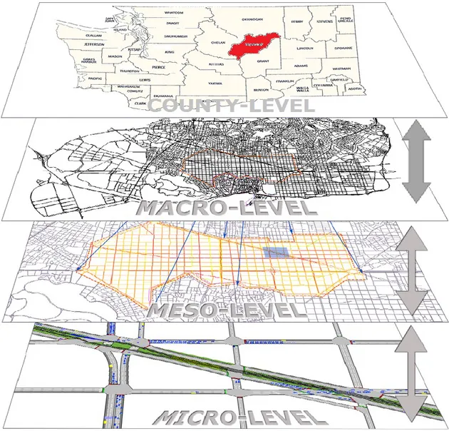
A review of the literature related to the previous studies showed that traffic safety studies mainly divided into four different levels including county-level, macro-level, meso-level, and micro level (see Fig. 1.1). In the county-level crash risk analysis, traffic accident counts are aggregated in order to relate traffic safety to a series of countywide factors such as road network attributes, socio-demographic characteristics, socioeconomic variables, road infrastructure variables, income, GDPs, trip generation and distribution, traffic patterns etc. Macro-level model is useful for analyzing crash data at large geographic areas, such as metropolitan area. Meso-level models generally analysis safety performance of zones in a city (focuses on zonal-level) or considers segments of major arterial roadways within the city boundary. Micro-level model is appropriate for smaller aspects of a network (specific roadway entities) such as an interchange, roadway segments, specific corridors, etc.

Most of the existing research focused only on county, meso, and micro levels of traffic safety analysis. These models are usually appropriate for traffic safety analysis due to the detail of

5

information provided and models give more accurate results than macro-level. These models are rarely used to investigate the safety performance of traffic counts in a large geographic area such as an entire metropolitan area (macro-level), mainly because of the difficulty in assembling the large amount of detailed information and significant computational cost. However, macro-level safety analysis can more efficiently detect problems in a larger area and it is suitable for helping establish long term planning policy to improve road safety. In this study, we focused only on traffic safety analysis at macro-level.

6

In addition, the sole study on road traffic safety in Sherbrooke is Vandersmissen (1995). In the subsequent years, the number of road users has increased rapidly, which translates into a higher risk of drivers being injured or killed in road accidents. According to 2011 crash-rate information, Sherbrooke had a higher average fatality rate than Quebec or Canada. Consequently, it is crucial to find a way in order to determine crash patterns and identify hazardous locations throughout the network.

1.3 Objective

In this study, we defined a site as a hotspot location where traffic crashes have been recurrently or consecutively concentrated. Therefore, the primary objective of this research was to identify hotspots based on a historical crash data set and spatiotemporal patterns of traffic accidents in order to improve road safety. Knowing the locations of hotspots and how to avoid them can help reduce the number of collisions in urban areas. The main objectives of this research were:

 Show how taking the exposure (traffic-volume) data into account affects hotspot identification.

 Demonstrate that the combined results obtained from spatial-data analysis using the network-KDE method and the results obtained using the HSM technique are suitable for identifying hotspot locations.

 Investigate the relation between different seasons and the number of crashes based on spatial and temporal analyses.

 Examine the influence of various seasons (different weather conditions) on the distribution of collision severity.

7

In order to achieve these objectives, GIS-based spatial analysis, spatiotemporal analysis with the CoMap method, and significance test methods were implemented with a focus on vehicle traffic accidents.

1.4 Hypotheses

The following hypotheses are discussed in this study:

 Hypothesis I: Hotspot locations are expected to be concentrated around intersections or

junctions. This is due to the higher density of road users such as motorists, cyclists, and pedestrians encountered daily at intersections.

 Hypothesis II: Traffic-accident patterns are expected to differ from one season to another.

Weather is a significant environmental factor that affects crash rates. For instance, weather conditions—especially snow and rain—represent a serious risk factor for road safety, and the risk of crashes increases during precipitation.

1.5 Limitations

Our study only considered vehicle-to-vehicle traffic accidents for hotspot analysis. Other types of accidents—including vehicle-to-pedestrian and vehicle-to-cyclist accidents—are beyond our scope. We focused on safety analysis in urban areas and considered all types of public roadways, such as arterial, collector, and local roads within city limits, excluding highways, interchanges, private roads, and parking lots.

Neither did our study distinguish between daytime and nighttime traffic accidents, because they have different characteristics. Nighttime traffic accidents mainly happen due to lighting, driver drowsiness, or inadequate signage, while daytime traffic accidents occur due to other factors such as road geometry and driver behavior.

8

1.6 Thesis Contributions

Limitations observed in the literature suggest the need to address new methods for identifying crash hotspot locations on a roadway network. In this study, the first article differs from the previous research activities (spatial analysis of traffic accidents) by considering the traffic volume data as an exposure, which addresses this issue at a macro-level data structure. Traffic volume is an important data particularly when comparing sites/sections with widely ranging traffic volumes. This method also divide the selected hazardous locations/site into different homogenous reference-

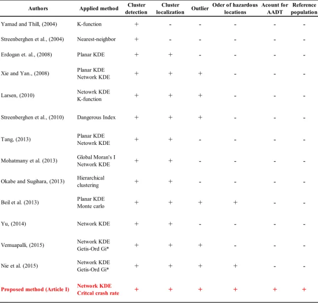
Table 1.1 Comparison with other methods (article I)

Authors Applied method Cluster detection Cluster localization Outlier Oder of hazardous locations Acount for AADT Reference population

Yamad and Thill, (2004) K-function + - - - -

-Streenberghen et al., (2004) Nearest-neighbor + - - - -

-Erdogan et. al., (2008) Planar KDE + + - - -

-Xie and Yan., (2008) Planar KDE

Network KDE + + + - -

-Larsen, (2010) Netowrk KDE _K-function + + + - -

-Streenberghen et al., (2010) Dangerous Index + + + - -

-Tang, (2013) Planar KDE

Netowrk KDE + + - - -

-Mohatmany et al. (2013) Global Moran's I

Network KDE + + - - -

-Okabe and Sugihara, (2013) Hierarchical

clustering + + - - -

-Beil et al. (2013) Planar KDE

Monte carlo + + + + -

-Yu, (2014) Network KDE + + - - -

-Vemuapalli, (2015) Network KDE _{Getis-Ord Gi*} + + + - -

-Nie et al. (2015) Network KDE _{Getis-Ord Gi*} + + + + -

-Proposed method (Article I) Network KDE

Critcal crash rate + + + + + +

9

populations based on intersections configuration (signalized or unsignalized intersections, three legs or four legs intersections) or segments configuration (two lanes or three lanes roadway segments). To show the contribution of our method, we also compared our study with other researches which were used in cluster analysis of crashes based on different factors including cluster detection, cluster localization, outlier, order of hazardous locations, account for AADT, and reference population (See Table 1.1).

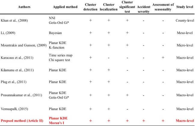
In the second article, to show the contribution of the proposed method, we provided a comparison with other methods, which used in spatiotemporal analysis of traffic accidents. The comparison shows that our method improves the spatiotemporal analysis of traffic accidents by taking into account crash severity and assessment of seasonality at macro-level (See Table 1.2).

Table 1.2 Comparison with other methods (article II)

Authors Applied method Cluster

detection Cluster localization Cluster significant test Accident severity Assessment of

seasonality Study level

Khan et al., (2008) NNI _{Getis-Ord Gi*} + + + - - County-level

Li, (2009) Bayesian + + + - - Meso-level

Mountrakis and Gunson, (2009) Planar KDE

K-function + + + - - Micro-level

Karacaus et al., (2011) Time series map

Chi square test + - - - + Macro-level

Kilamanu et al., (2011) Planar KDE + + - - - Macro-level

Plug et al., (2011) Planar KDE + + - - - Macro-level

Prasannakumar et al., (2011) Planar KDE

Getis-Ord Gi* + + + - - Macro-level

Vemuapalli, (2015) Planar KDE + + - - - Macro-level Propsed method (Article II) Planar KDE _{Moran's I} + + + + + Macro-level

10

1.7 Thesis Structure

As part of this research, we have written two articles that have been (first article) or will be published (second article) in scientific journals (peer-reviewed journal) in the field of traffic safety and transport geography. Hence, our research is presented herein as a thesis by publication.

In this chapter, we presented the background and research problems (issues relevant to traffic safety) including the research objectives and hypotheses. The rest of the thesis is organized as follows. Literature review and study data are explained in chapters 2 and 3. Chapters 4 and 5 are the two scientific papers written on this research. Each of these chapters begins with a discussion of the background, methods, and scientific scope of the article, followed by the original text of the article. The sixth chapter provides a general discussion. The final chapter consists of the overall conclusion as well as recommendations and prospects.

11

2. Literature Review

This section contains a review of the literature related to the previous studies on road safety analyses in many perspectives. Road network safety analysis include statistical models, which can be applied to explain the variability in the safety performance measure. In reality, numerous factors contribute to occurrence of traffic crashes. However, some of the relevant factors are not observable because they are latent or difficult to obtain. Hence, missing some of the relevant factors leads to unobserved heterogeneity, which shows the effect of all unobserved factors. In other words, when an accident influencing factors cannot be calculated and estimated properly, it leads to unobserved heterogeneity. In fact, it neglects significant information in explaining the observed crash frequency (Mulokozi, 2015).

The first section (2.1) introduces previous spatial, temporal, and spatial-temporal (spatiotemporal) analyses of traffic accidents. Non-spatial models such as hotspot analyses methods, crash prediction models, Bayesian approach, observed heterogeneity counts modeling, and unobserved heterogeneity counts modeling are summarized in sections 2.2 to 2.4. The last section indicates the limitations in the current literature that this study is trying to fill.

2.1 Spatial Modeling

Traffic accidents have been studied from various temporal and spatial perspectives. Concerning the temporal patterns of traffic accidents, several studies investigated on traffic accidents frequency according to different temporal scales, such as hourly, daily, monthly and yearly (Karacasu et al., 2011; Brown and Baass, 1997; El-Sadig et al., 2002; Bačkalić, 2013; Levin et al., 1995b). The main difference between spatial and temporal analysis is that spatial analysis is based on counting number of crashes on a define space while temporal analysis is based on time series and required positioning and tracking occurrences of traffic accidents in dynamic dimension.

12

Traffic accidents must be analyzed in order to reduce the number of traffic fatalities and injuries. Many road authorities currently use complex statistical methods for exploring hotspot locations. Most traditional approaches focus on the time dimension of traffic accidents, and standard statistical techniques are used to assess spatial patterns. In recent years, the use of the spatial dimension of point events referred to as point-pattern analysis has increased dramatically. The first application of GIS in traffic-safety analysis was carried out in 1976. Since then, various studies have been conducted and methods used in analyzing traffic accidents, ranging from simple methods (such as mapping) to advanced ones (such as spatial statistical analysis).

The objective of point-pattern analysis is to determine whether point events (traffic accidents) in an area have a spatial dependency (clustering) or if they are randomly distributed. In general, point-pattern analysis is classified according to two primary purposes: exploring first- and second-order properties. The former estimates how traffic-accident intensity varies across a region. In fact, it measures intensity based on the density or mean number of traffic accidents in a region. It includes techniques such as KDE and quadrat analysis, which have been used to identify clustering patterns of traffic accidents. The second group, however, estimates the presence of spatial dependency among traffic accidents based on the distances between them. Exploratory spatial statistical methods such as the nearest-neighbor distance, K-function, quadrat analysis, and Moran’s I have been used for measuring the spatial dependency of traffic accidents. Table 2.1 lists the main publications related to identifying the spatial clustering of traffic accidents.

Of the various techniques that have been applied in identifying the spatial dependency (second order) of traffic accidents, the nearest-neighbor distance figures prominently in the literature. For instance, Levine et al. (1995a) used the nearest-neighbor distance approach and found a significant cluster of traffic accidents in Honolulu. Other common second-order techniques include Moran’s I (Loveday, 1991;Black and Thomas, 1998), quadrat analysis (Nicholson, 1999), and Ripley’s K-function (Okabe and Yamada, 2001;Yamada and Thill, 2004). Although second-order measures help estimate the presence of spatial dependency among traffic accidents, they fail to identify

13

traffic-accident clusters within the entire study area and overestimate cluster of traffic accidents (Lu and Chen, 2007; Yamada and Thill, 2004). As identifying traffic-accident clusters (risk-prone areas) is meaningful in road-safety studies, our study focused on first-order properties and statistical approaches for detecting clusters of traffic accidents.

The first-order property can be divided into two subgroups based on whether traffic accidents are treated as planar or network constrained (Yamada and Thill, 2004). The planar methods assume that the distance between traffic accidents (point events) is calculated according to the Euclidean (or straight-line) distance in a continuous planar space (Yao et al., 2015). As traffic accidents can occur only on a road network and retail facilities, such as gas stations, planar methods may not be suitable due to their assumption of one-dimensional space (Yao et al., 2015; Yamada and Thill, 2004). Therefore, some researchers have replaced planar methods with network-constrained methods in which the distance between traffic accidents is usually calculated based on shortest path along the network.

KDE is a technique that has been widely used in first-order properties to identify traffic-accident hotspots. In the early phase, planar KDE was used to identify hotspot locations (Steenberghen et al., 2004;Sabel et al., 2005;Erdogon et al., 2008;Anderson, 2009;Chung et al., 2011;Plug et al., 2011). For instance, Sabel et al. (2005) used planar KDE to identify hotspot locations in Christchurch, New Zealand. The results show that the method can identify traffic-accident clusters.

Steenberghen et al. (2004) used planar KDE for traffic-accident clustering in an urban area and found that planar KDE was suitable for dense networks with dispersed traffic accidents. Erdogon et al. (2009) applied a planar KDE method to explore the collision hotspot locations on Turkish roads.

14

Table 2.1 Selected publications related to identifying the spatial clustering of traffic accidents by type of spatial

statistic

Methods Publications Year Type of Spatial Statistic

Second order

Clark and Evans 1954

Nearest-neighbor index Stark and Young 1981

Levine et al. 1995a

Okabe and Sugihara 2012

Nicholson 1999 Quadrat methods

Okabe and Yamada 2001

Ripley’s K-function Yamada and Thil 2004

Loveday 1991

Moran’s I Black and Thomas 1998

First order Flauhaut et al. 2003 Planar KDE Sabel et al. 2005 Erdogon et al. 2009 Anderson 2009 Chung et al. 2011 Plug et al. 2011 Thakali et al. 2015

Xie and Yan 2008

Network-constrained KDE Okabe et al. 2009 Steenberghen et al. 2010 Sugihara et al. 2010 Loo et al. 2011 Bil et al. 2013

Xie and Yan 2013

Mohaymany et al. 2013

Young and Park 2014

Nie et al. 2015

Steenberghen et al. 2004

Planar and network KDE Yamada and Thill 2004

Borruso 2008

Larsen 2010

15

With planar KDE, the whole region is divided into grids of equal cell size. A kernel function is applied to calculate the density of collisions within a predefined search radius (Yao et al., 2015). This method, however, has a significant limitation: in the case of crashes occurring within a road network (one-dimensional space), an assumption of two-dimensional space does not hold (Xie and Yan, 2008). Accordingly, different studies have tried to overcome these limitations by extending the planar method into network space. In an early phase, Xie and Yan (2008) proposed a network-constrained method based on KDE to identify traffic-accident hotspots. Okabe et al. (2009)

proposed a network-constrained kernel called “equal split discontinuous function at nodes” to calculate the density of point events along a network. In addition, some studies have compared the results of hotspot analysis using planar- and network-KDE approaches (Borruso, 2008;Kuo et al., 2011;Larsen, 2010;Steenberghen et al., 2004;Yamada and Thill, 2004). Their results show the advantages of network KDE. Nonetheless, a major drawback of both planar and network KDE is the lack of statistical significance of the high-density locations. Therefore, the significance (robustness) of clusters must be tested more objectively. The local Moran’s I statistics introduced by Anselin (1995) and local G statistics introduced by Getis and Ord (1992) are two well-known methods conducted to test the significance of clusters (Bíl et al., 2013;Jeefoo et al., 2011;Xie and Yan, 2013; Nie et al., 2015). Our research used the local Moran’s I to significantly test for the detection of clusters.

Traffic-safety engineers realize that weather conditions, in the form of snow, rain, fog, wind, or ice, inevitably affects road safety throughout the year (Khan et al., 2008). Therefore, it is crucial for traffic-safety engineers to identify the accurate location (spatially) and time (temporally) of these traffic accidents. Few studies, however, have investigated the spatiotemporal aspects of point patterns. In the early phase, researchers used map animation techniques to represent spatiotemporal patterns (Moellering, 1976;Tobler, 1970;Dorling, 1992). Some other researchers used isosurface methods to integrate two-dimensional space and the time dimension (Whitaker et al., 2005; Brunsdon et al., 2007). Brundson (2001) proposed the CoMap technique to illustrate how the spatial

16

patterns of point events vary over time. This technique has been used in various spatiotemporal studies other than traffic safety such as in the health field (Getis and Ord, 1992;Jeefoo et al., 2010; Bhunia et al., 2013), analysis of oil spills (Park et al., 2016;Meng, 2016), crime analysis (Wang et al., 2016), and fire analysis (Corcoran et al., 2007;Asgary et al., 2010;Ceyhan et al., 2013;Yao and Zhang, 2016). The technique has also been used in some traffic-safety studies (Barnao, 2009; Erdogan, 2009;Plug et al., 2010;Kilamanu et al., 2011; Prasannakumar et al., 2011;Kuo et al., 2011). For these studies, the researchers used various spatial methods such as KDE, Moran’s I, and

Gi* statistics to identify time-related hotspots.

2.2 Non-Spatial Modeling

This section reviews non-spatial modeling of roadways. Non-spatial modeling includes only the mathematical association of accident frequency with traffic, geometric, driver behaviors, environmental characteristics of a roadway network without involving its spatial effect (Mulokozi, 2015). In this case, the accident frequency of a roadway is assumed to be described by non-spatial characteristics such as geometry design or driver behaviors, which do incorporate spatial characteristics such as distance or spatial matrices.

Many local transportation agencies in North America, especially those in urban areas, use network-screening performance measures to identify hotspot locations/sites (Young and Park, 2014). Numerous network-screening performance methods are available from various sources, including the Highway Safety Manual (HSM) (AASHTO, 2010) and the Highway Safety Improvement Program Manual (HSIPM) (Herbel et al., 2010). However, many of these methods are appropriate for micro-level and meso-level of safety analysis because they need an intensive input data.

17

2.2.1 Accident Frequency

Accident frequency is the oldest and simplest method to identify road safety shortages, summarizes the number of accidents for each location, and ranks them by descending order. Those locations with higher than predetermined number of accidents are classified as a high-frequency location/site. This method is useful for identification hotspot locations. However, this method does not take into consideration traffic exposure (traffic volume is the most commonly used traffic exposure unit), which has a direct relationship with accident frequency. Therefore, the results have bias toward high-volume locations/sites (Li, 2006). Also, this method does not consider accident severity (PIARC, 2003; AASHTO, 2010).

2.2.2 Crash Rate Method

The crash rate method ranks locations/sites using a ratio between number of traffic accidents and traffic volume (as a traffic exposure). For information, traffic volume at intersections is determined using the sum of entering number of vehicles. On roadways segments, traffic volume is calculated by adding up vehicles travelling in both directions. The advantage of this method is that it takes into account traffic exposure. The problem is that it does not consider the random nature of traffic accidents. It also assumes a linear relationship between number of traffic accidents and traffic volume; this may be a source of error. The method suffers from the regression-to-the-mean (RTM) bias in which an artificial high crash rate is likely to decrease subsequently even without improvement to the site (PIARC, 2003; AASHTO, 2010; Li, 2006).

2.2.3 Critical Crash Rate Method

The critical crash rate method identifies those locations/sites where crash rate is greater than the average crash rate for similar sites across the state or similar region (Li, 2006). This method also compares the crash rate at a location with the average crash rate of similar sites having similar characteristics. The basis assumption is that similar sites should have similar safety level.

18

The advantages of this method is that it takes into account the random nature of traffic accidents as well as traffic exposure. However, this method does not consider accident severity and suffers from the RTM bias (PIARC, 2003; AASHTO, 2010).

2.2.4 Equivalent Property Damage Only Method

The Equivalent Property Damage Only (EPDO) method assigns a weight to each accident by severity (Property Damage Only – PDO, injury, fatal) in order to develop a combined frequency and severity score per location/site (AASHTO, 2010). The weighting factors are calculated relative to the property damage only accidents. Various weighting factors have been proposed such as monetary values (AASHTO, 2010), weighting factors (Agent, 1973), etc. For example, Agent (1973) assigned a weight of nine to fatal crash and serious injury crashes, a weight of three to minor injury crashes, and a weight of one to PDO crashes.

Unlike previous methods, the method takes into account accident severity. However, this method does not consider for traffic exposure and it has bias towards high-speed locations/sites and suffers from the RTM bias (PIARC, 2003; AASHTO, 2010; Li, 2006).

2.2.5 Relative Severity Index Method

The relative severity index method assigns a weight (crash costs) to each traffic accident at each location related to the crash type. In this method, an average RSI accident cost is estimated for each location/site and for each reference population. Sites are ranked based on their average RSI cost (AASHTO, 2010; Li, 2006). This method has the same limitations as the EPDO method.

2.3 Crash Prediction Models

As stated earlier, the objective of the methods described in the previous section is to identify those locations/sites have an abnormal crash consideration. However, these methods do not calculate the differences in safety between the location/site and the average accident frequency (reference population). In practice, it is difficult (or may be impossible) to accurately measure the

19

average crash frequency when a sufficient number sites having similar characteristics cannot be found. Hence, the development of crash prediction models may reduce this problem by estimates number of crashes based on function of independent variables (PIARC, 2003). Moreover, prediction models take into account the effect of geometric road features on crash occurrence by developing numerous forms of crash prediction models, so called as Safety Performance Function (SPF).

Numerous forms of crash prediction models using SPF have been proposed in the literature such as Level of Service of Safety (LOSS), Excess Predicted Average Crash Frequency Using SPFs.

2.3.1 Level of Service of Safety (LOSS)

The level of service of safety method uses a SPF in order to compare the observed accident frequency/severity to the mean value for the reference population. The difference between the two values indicates a low/high potential for crash reduction.

The advantages of this method is that it considers variance in accident data, establishes a threshold for comparison. However, this method does not consider RTM bias as well as traffic volumes (AASHTO, 2010).

2.3.2 Excess Predicted Average Crash Frequency Using SPFs

The excess predicted average crash frequency using SPFs method shows the difference between the observed accident frequency for the site and predicted accident frequency based on SPF. This method accounts for traffic volume and establishes a threshold value for comparison between the observed and predicted crash frequency. The problem of this method is that it requires calibrated SPF and effects of RTM bias may still be present in the results (AASHTO, 2010).