Variability in the super-Earth 55 Cnc e

arXiv:1505.00269v2 [astro-ph.EP] 20 Nov 2015

Variability in the super-Earth 55 Cnc e

Brice-Olivier Demory

, Michael Gillon

, Nikku Madhusudhan

& Didier Queloz

1_{Astrophysics Group, Cavendish Laboratory, J.J. Thomson Avenue, Cambridge CB3 0HE, UK.}

2_{Institut d’Astrophysique et de G´eophysique, Universit´e of Li`ege, all´ee du 6 Aout 17, B-4000 Li`ege, Belgium.} 3_{Institute of Astronomy, University of Cambridge, Cambridge CB3 0HA, UK.}

Accepted 2015 September 25. Received 2015 September 23; in original form 2015 March 10

ABSTRACT

Considerable progress has been made in recent years in observations of atmospheric signa-tures of giant exoplanets, but processes in rocky exoplanets remain largely unknown due to major challenges in observing small planets. Numerous efforts to observe spectra of super-Earths, exoplanets with masses of 1-10 Earth masses, have thus far revealed only featureless spectra. In this paper we report a 4-σ detection of variability in the dayside thermal emis-sion from the transiting super-Earth 55 Cancri e. Dedicated space-based monitoring of the planet in the mid-infrared over eight eclipses revealed the thermal emission from its day-side atmosphere varying by a factor 3.7 between 2012 and 2013. The amplitude and trend of the variability are not explained by potential influence of star spots or by local thermal or compositional changes in the atmosphere over the short span of the observations. The possi-bility of large scale surface activity due to strong tidal interactions possibly similar to Io, or the presence of circumstellar/circumplanetary material appear plausible and motivate future long-term monitoring of the planet.

Key words: stars: individual: 55 Cnc – techniques: photometric

1 INTRODUCTION

A key question in exoplanet science is about the origin of planets in tight orbit (P<0.75 days) around their stars. During its primary mis-sion, Kepler enabled the detection of a hundred ultra-short period (USP) planet candidates (Sanchis-Ojeda et al. 2014). The majority of these USP planets are small (RP < 2R⊕) and may suggest that they have experienced a phase of intense erosion due to tidal activ-ity and/or intense stellar irradiation (e.g.Owen & Wu 2013).

One example of these disintegrating USP planets is KIC12557548b (Rappaport et al. 2012), which exhibits changes in the optical transit depth and shape that seem consistent with an evolving cometary-like environment (Brogi et al. 2012;

Rappaport et al. 2014; Croll et al. 2014; Bochinski et al. 2015).

Scattering of dust particles surrounding the planet are thought to be the driver of the observed variability, as the engulfed sub-Mercury-size object itself would be too small to be actually de-tected (Perez-Becker & Chiang 2013). The high effective tempera-tures of USP planets could enable a silicate-rich atmosphere made of refractory material to be sustained, which would shape the over-all opacity. Replenishment of grains in the atmosphere could be achieved by condensation at cooler temperatures near the day-night terminator or at lower pressures (Schaefer & Fegley 2009;

Castan & Menou 2011). Another source for the observed refractory

material could be volcanism, fuelled by tidal heating (Jackson et al.

2008;Barnes et al. 2010) similar to Io, where the interactions

be-⋆ _{E-mail: bod21@cam.ac.uk}

tween an inhomogeneous circumplanetary neutral cloud and a cir-cumstellar charged torus (Belcher 1987) would result in transit depth variability over timescales that are similar to the planet’s or-bital period.

The super-Earth 55 Cancri e has a mass of8.09 ± 0.26 M⊕

(Nelson et al. 2014), a published radius of 2.17 ± 0.10 R⊕

(Gillon et al. 2012), and orbits a nearby sun-like star with an

18-hour period. 55 Cnc e is one of the largest members of known USP planets. Owing to its close proximity to the parent star, 55 Cnc e has an equilibrium temperature of ∼2400 K and may experience intense tidal heating (Bolmont et al. 2013_{). With V∼6, 55 Cnc}

is the brightest star known to host a transiting exoplanet, and has led to measurements of the planet’s radius at exquisite preci-sion in the visible as well as in the Spitzer 4.5µm IRAC band

(Demory et al. 2011;Winn et al. 2011;Gillon et al. 2012).

Ther-mal emission measurements in the Spitzer 4.5µm IRAC photo-metric band (Demory et al. 2012) yielded a brightness temperature of about 2,300 K in this channel. Such elevated temperature has implications on the nature of the planet atmosphere. First, this high temperature means that for a given chemical composition, 55 Cnc e would have a larger atmospheric scale height compared to a cooler planet with the same composition. Second, clouds are less likely to form in the atmospheres of extremely hot exoplanets compared to cooler objects (Madhusudhan & Redfield 2015), which is particu-larly relevant in the light of the numerous non-detections of spec-tral features in exoplanets (e.g.Pont et al. 2008;Sing et al. 2011;

Knutson et al. 2014;Kreidberg et al. 2014). The combination of the

obser-vations and the high planetary temperature means that 55 Cnc e currently represents one of the most promising super-Earth for in-frared spectroscopic observations of its atmosphere. Using the pub-lished mass and radius alone, the interior composition of the planet is consistent with: (1) a silicate-rich interior with a dense H2O en-velope of 20% by mass (Demory et al. 2011), (2) a purely silicate planet with no envelope (e.g.Gillon et al. 2012), or (3) a carbon-rich planet with no envelope (Madhusudhan et al. 2012) among other compositions.

In this paper, we present an analysis of archival and new Spitzer/IRAC data obtained in 2012 and 2013. This combined dataset suggests a radically different nature for 55 Cnc e that could be more consistent with a scenario similar to KIC12557548b than the more conventional picture that was attached to 55 Cnc e and which is described above. We present the observations and data analysis in Section 2, a comparison with previous results in Sec-tion 3 and we finally propose an interpretaSec-tion of our results in Section 4.

2 DATA ANALYSIS 2.1 Observations

This study is based on six transits and eight occultations of the super-Earth 55 Cnc e acquired between 2011 and 2013 in the 4.5-µm channel of the Spitzer Space Telescope (Werner et al. 2004) Infrared Array Camera (IRAC) (Fazio et al. 2004). Data were ob-tained as part of the programs IDs 60027, 80231 and 90208. Two transits were observed in 2011 (PID 60027) (Demory et al.

2011;Gillon et al. 2012), four occultations in 2012 (PID 80231)

(Demory et al. 2012), as well as four transits and four other

oc-cultations in 2013 (PID 90208). The corresponding data can be accessed using the Spitzer Heritage Archive1_{. All Spitzer} obser-vations have been obtained with the same exposure time (0.02 s) and observing strategy (stare mode). The last three occultations of PID 80231 have been obtained using the PCRS peak-up mode as all of our 2013 data. The PCRS peak-up procedure is designed to place the target on a precise location on the detector to mitigate the intra-pixel sensitivity (Ingalls et al. 2012, and references therein). The AORs 48072704 and 48072960 experienced 30-min long inter-ruptions that happened during the ingress and egress of 55 Cnc e’s transit respectively.

2.2 Data reduction

The starting point of our reduction consists of the basic calibrated data (BCD) that are FITS data cubes encompassing 64 frames of 32x32 pixels each. Our code sequentially reads each frame, con-verts fluxes from the Spitzer units of specific intensity (MJy/sr) to photon counts, and transforms the data timestamps from BJDUTC to BJDTDB(Eastman et al. 2010). The position on the detector of the point response function (PRF) is determined by fitting a Gaus-sian to the marginal X, Y distributions using theGCNTRD pro-cedure part of the IDL Astronomy User’s Library2. We also fit a two-dimensional Gaussian to the stellar PRF (Agol et al. 2010). We find that determining the centroid position usingGCNTRD re-sults in a smaller dispersion of the fitted residuals by 10 to 15%

1 _{Spitzer Heritage Archive: http://sha.ipac.caltech.edu} 2 _{IDL Astronomy User’s Library: http://idlastro.gsfc.nasa.gov}

across our dataset, in agreement with other warm Spitzer analy-ses (Beerer et al. 2011). We then perform aperture photometry for each dataset using a modified version of theAPER procedure using aperture sizes ranging from 2.2 to 4.4 pixels in 0.2 pixels intervals. The background apertures are located 10 to 14 pixels from the pre-determined centroid position. We also measure the PRF full width at half maximum along the X and Y axes. We use a moving av-erage based on forty consecutive frames to discard datapoints that are discrepant by more than 5σ in background level, X-Y position and FWHM. In average, we find that 0.5% of the datapoints ac-quired without the PCRS peak-up mode are discarded, while it is only 0.06% when the PCRS peak-up mode is enabled. The result-ing time-series are finally binned per 30 s to speed up the anal-ysis. The product of the data reduction consists of a photometric datafile for each aperture (12 in total per dataset). We then use the out-of-eclipse portion of the light curve to measure the RMS and level of correlated noise (see Sect.2.3.2) to determine the aperture that minimises both quantities. In the cases of AORs 48070144, 48073472 and 48073728 we found that two to three aperture sizes produced similarly small RMS and beta factors. We selected the one with the smallest RMS. For these three AORs, repeating the analysis using the other aperture sizes does not change the retrieved occultation depths. We show the retained aperture size as well as the corresponding RMS andβ factor for each dataset in Table1. For all datasets we discard the photometry corresponding to the first 30 minutes as it usually exhibits a strong time-dependent ramp

(Demory et al. 2011). This procedure is common practice for warm

Spitzer data (e.g.Deming et al. 2011).

2.3 Photometric Analysis

We split the analysis in three steps. In a first step we focus on the modelling of the intra-pixel sensitivity and the photometric preci-sion. The second step focuses on an improved determination of the system parameters using six transits and eight occultations. The third step details the analysis focusing on the variations in transit and occultation depths.

2.3.1 Intra-pixel sensitivity correction

Warm Spitzer data are affected by a strong intra-pixel sensitiv-ity that translates into a dependence of the stellar centroid posi-tion on the pixel with the measured stellar flux at the 2% level

(Charbonneau et al. 2005). A usual method is to detrend the

mea-sured flux from the X/Y position of the centroid, using quadratic order polynomial functions. In the past years, several stud-ies (Ballard et al. 2010;Stevenson et al. 2012;Lewis et al. 2013;

Deming et al. 2014) have employed novel techniques that improved

the mitigation of the intra-pixel sensitivity in Spitzer/IRAC 3.6 and 4.5µm channels.

It has been shown that in some cases, the technique used to correct the intra-pixel sensitivity could have a significant impact on the retrieved system parameters in general and the eclipse depth in particular (Deming et al. 2014). In the present work, we use a mod-ified implementation of the BLISS (BiLinearly-Interpolated Sub-pixel Sensitivity) method (Stevenson et al. 2012).

The BLISS algorithm uses a bilinear interpolation of the mea-sured fluxes to build a pixel-sensitivity map. The data are thus self-calibrated. We include this algorithm in the Markov Chain Monte Carlo (MCMC) implementation already presented in the litera-ture (Gillon et al. 2012). The improvement brought by any pixel-mapping technique such as BLISS requires that the stellar centroid

Date [UT] Program ID AOR # AOR duration [h] Eclipse type Aperture [pix] RMS/30s [ppm] βr 2011-01-06 60027 39524608 4.9 Transit 2.6 359 1.75 2011-06-20 60027 42000384 5.9 Transit 3.2 367 1.45 2012-01-18 80231 43981056 5.9 Occultation 2.8 364 1.54 2012-01-21 80231 43981312 5.9 Occultation 3.2 329 1.04 2012-01-23 80231 43981568 5.9 Occultation 3.2 337 1.00 2012-01-31 80231 43981824 5.9 Occultation 3.2 362 1.27 2013-06-15 90208 48070144 5.9 Occultation 2.6 323 1.12 2013-06-21 90208 48070656 8.8 Transit 2.8 365 1.88 2013-07-03 90208 48072448 8.8 Transit 3.2 350 1.16 2013-07-08 90208 48072704 8.8 Transit 2.6 378 1.37 2013-07-11 90208 48072960 8.8 Transit 2.6 400 1.85 2013-06-18 90208 48073216 8.8 Occultation 3.0 325 1.59 2013-06-29 90208 48073472 8.8 Occultation 3.0 357 1.33 2013-07-15 90208 48073728 8.8 Occultation 3.4 381 1.25

Table 1. 55 Cnc e Spitzer dataset. Astronomical Observation Request (AOR) properties for 2011-2013 Spitzer/IRAC 4.5-µm data used in the present study.

remains in a relatively confined area on the detector, which warrants an efficient sampling of the X/Y region, thus an accurate pixel map. In our implementation of the method, we build a sub-pixel mesh made ofn2

grid points, evenly distributed along thex and y axes. The BLISS algorithm is applied at each step of the MCMC fit. The number of grid points is determined at the beginning of the MCMC by ensuring that at least 5 valid photometric measurements are lo-cated in each mesh box. Similar toLanotte et al.(2014), we find that the PRF’s FWHM along thex and y axes evolve with time and allows further improvement on the systematics correction. We thus combine the BLISS algorithm to a linear function of the FWHM along each axis. We find that including a model of the FWHM de-creases the Bayesian Information Criterion (BIC,Schwarz 1978) for all datasets. Including a linear dependence with time does not improve the fit. We find no correlation between the photometric time-series and the background level. We finally perform the same intra-pixel sensitivity correction using a variable aperture in the re-duction and including the noise pixel (Lewis et al. 2013) parameter as an additional term in the parametric detrending function. As no-ticed in previous studies (Lewis et al. 2013), we find this approach slightly increases the BIC in the 4.5µm channel. We repeat this part of the analysis with lightcurves using apertures sizes smaller and larger by 0.2 pixels from the one minimising the photometric RMS. We subtract the lightcurves using the altered aperture sizes to the optimal one and find point-to-point variations embedded in the 1-σ individual error bars. We further check the incidence of binning on the efficiency of the intra-pixel sensitivity correction by analysing the 2012-01-18 occultation (obtained with the PCRS mode enabled) with binnings ranging from 0.64s (one integrated subarray data cube), 6s, 12s and 30s. We find the following depths: 106±55, 91±57, 111±60 and 87±53 ppm respectively. We thus conclude that using binnings up to 30s does not affect the occulta-tion depth measurement.

2.3.2 Noise budget and photometric precision

The data reduction described above computes the theoretical er-ror for each photometric datapoint. In order to derive accurate un-certainties on the parameters, we evaluate the level of correlated noise in the data following a time-averaging technique detailed in

Pont et al.(2006). We compute within the MCMC fit a correction

factorβ based on the standard deviation of the binned residuals for each light curve using different time-bins. We keep the largest cor-rection factorβ found for each dataset and multiply the theoretical

errors by this factor. We show on Table1the photometric RMS and β for each dataset. We also conduct a residual permutation boot-strap analysis to obtain an additional estimation of the residual cor-related noise. We use for this purpose the lightcurve corrected from the systematic effects described in Sect.2.3.1. The resulting pa-rameters are in agreement with the ones derived from the MCMC analysis (Table2), while their error bars are significantly smaller. This result indicates that the error budget is dominated by the base-line model uncertainties and not by the residual correlated noise.

2.3.3 Refinement of the system parameters

In the second step of our analysis, we use as input data to the MCMC all six transits and eight occultations. The goal of this part of the analysis is to refine the published parameters for the orbital and physical parameters of 55 Cnc e. The jump parameters are the planetary-to-star radius ratioRP/R⋆, the planetary impact param-eterb, orbital period P , transit duration W and centre T0, and the occultation depthδocc. In a first MCMC run, we keep the eccen-tricity fixed to zero as previous studies using radial-velocity data, which provides better constraints on√e sin ω, found eccentricity values consistent with 0 (Nelson et al. 2014). We also add the limb-darkening linear combinationsc1= 2u1+ u2andc2 = u1− 2u2 as jump parameters, whereu1andu2are the quadratic coefficients drawn from the theoretical tables ofClaret & Bloemen(2011) us-ing published stellar parameters (von Braun et al. 2011). We im-pose Gaussian priors on the limb-darkening coefficients and the radial-velocity semi amplitude K (Nelson et al. 2014). We exe-cute two Markov chains of 100,000 steps each and assess their efficient mixing and convergence using the Gelman-Rubin statis-tic (Gelman & Rubin 1992) by ensuring r < 1.01. Results for this MCMC fit are shown on Table2. In a second MCMC run, we explore what limits can be placed on the orbital eccentricity e and argument of periastron ω. We perform a fit with√e cos ω and√e sin ω as additional free parameters and find√e cos ω = 0.01+0.04_−0.04 and √e sin ω = −0.05+0.14−0.17, corresponding to a 3-sigma upper limit on the eccentricity ofe < 0.19. We do not detect variations in the transit or occultation timings.

2.3.4 Transit depth variations

In this third part of the analysis, we assess whether transit depths vary across our 2011-2013 datasets. This MCMC fit includes the

Planet/star area ratioRp/Rs 0.0187+0.0007−0.0007

b = a cos i/R⋆[R⋆] 0.36+0.07_−0.09

T0− 2,450,000 [BJDTDB] 5733.008+0.002_−0.002

Orbital semi-major axisa [AU] 0.01544+0.00009_−0.00009

Orbital inclinationi [deg] 83+2−1 Mean densityρp[g cm−3] 6.3+0.8−0.7 Surface gravity loggp[cgs] 3.33+0.04_−0.04 MassMp[M⊕] 8.08+0.31_−0.31 RadiusRp[R⊕] 1.92+0.08−0.08

δocc(2012) [ppm] 47 ± 21

δocc(2013) [ppm] 176 ± 28

Table 2. 55 Cnc e system parameters. Results from the MCMC combined fit. Values indicated are the median of the posterior distributions and the 1-σ

corresponding credible intervals.

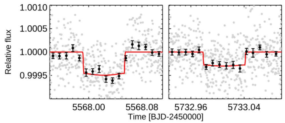
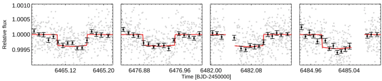
six transit lightcurves only, each of them having an independent planet-star radius ratioRP/R⋆. To increase the convergence effi-ciency, we use Gaussian priors onb, P , W and T0using the pos-terior distribution derived from the joint fit in the previous step. Results for this MCMC fit are shown on Table 3. The corrected lightcurves for each transit are shown on Fig. 1and 2while the corresponding correlated noise behaviour is shown on Fig.3and4. We find that 55 Cnc e’s transit depths at 4.5µm change by 25% in comparison to the mean value (365 ppm) between 2011 and 2013. Fitting all transits with a straight line yields a reduced chi-squared ofχ2

r = 1.2, corresponding to an overall variability sig-nificance of 1σ, which we consider being undetected. While most transit depth values are consistent at the 1-σ level, only the first 2011 transit appears as an outlier. Converting our transit depths to planetary sizes, we find a minimum planet radius of 1.75±0.13 Earth radii, a maximum radius of 2.25 ±0.17 Earth radii and an average value of 1.92±0.08 Earth radii. This value is significantly smaller than the published Spitzer+MOST combined estimate of 2.17 ±0.10 Earth radii (Gillon et al. 2012). Alternatively, these marginal transit depth variations could be due to steep variations of the stellar flux, which is however unlikely for this star (see Sect.2.5).

2.3.5 Occultation depth variations

In the following we assess the extent of variability in the planetary thermal emission. We first perform an MCMC fit that includes all eight occultations observed in 2012 and 2013, each of them having an individual depthδocc. All other parameters derived in Sect.2.3.3 are included as Gaussian priors in this MCMC fit. Results for this MCMC fit are indicated in Table4. The corrected lightcurves for each occultation are shown on Fig.5and6while the corresponding correlated noise behaviour is shown on Fig.7and8. Fitting all eight occultations with a straight line yields a mean occultation depth of 83±14 ppm and a corresponding χ2

r= 2.6.

In a second MCMC fit, we independently fit the occultations by season to investigate a difference in depth between 2012 and 2013. We find that fitting both the 2012 and 2013 occultation depth values with a straight line yieldsχ2

r= 13.6, meaning that constant occultation depths fits the data poorly at the 3.7-σ level. We find that the occultation depths as measured with Spitzer at 4.5µm vary by a factor of 3.7+4.1_{−1.6 between 2012 and 2013, from 47±21 to} 176±28 ppm. The resulting lightcurves for each season are shown on Fig.9and their posterior distributions on Fig.10. To interpret the variability in the occultation depth, we use an observed infrared spectrum of 55 Cnc (Crossfield 2012) to estimate the

correspond-ing change in the planet’s thermal emission. Assumcorrespond-ing a mean radius of 1.92 Earth radii, we find that between 2012 and 2013, the planet dayside brightness temperature at 4.5µm changes from 1365+219

−257K to2528 +224 −229K.

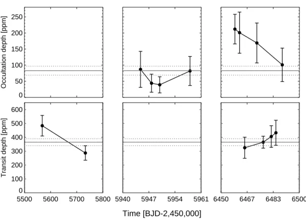
The time coverage of our combined 2011-2013 dataset (Fig.11) is too scarce to put firm constraints on the variability period of the emission and apparent size of 55 Cnc e, motivating further monitoring of this planet.

2.4 Discrepancy with the Demory et al. 2012 analysis

We investigate the discrepancy between our updated 2012 oc-cultation depth, 47±21 ppm, and our previous one published in

Demory et al.(2012_{), 131±28 ppm, assuming that the different}

models that we used in the two analyses are at the origin of the discrepancy. Indeed, in our 2012 work, we had not yet noticed the strong dependency of the measured fluxes on the measured widths of the PRF in thex and/or y directions. The improvement brought by the addition of the PRF FWHM in the baseline model is de-scribed in detail inLanotte et al.(2014) for the case of GJ 436. In 2012, our modelling of the Spitzer systematics was based uniquely on polynomials of the measuredx and y position of the PRF centre. Furthermore, to reach a decent level of correlated noise in the resid-uals of our fits, we had to add to our models quadratic functions of time and, for three occultations out of four, quadratic functions of the logarithms of time (Demory et al. 2012, Table 1). The resulting complex time-dependent models could have easily “twisted” the light curves to improve the fit, affecting the measured occultation depth by a systematic error. To test this hypothesis, we perform several MCMC analyses of the 2012 Spitzer light curves (as ob-tained with a photometric aperture of 3 pixels). For all these anal-yses, the transit parameters (depth, impact parameter, ephemeris) are kept under the control of Gaussian priors based on the result of our global analysis presented in Sect.2.3.3, and assuming a circular orbit.

In our first analysis (T1), we assume a common depth for all four 2012 occultations, and the same baseline models than in the present work (Sect.2.3.1) based on functions of the PRF centre position and widths. In our second test analysis (T2), we assume again a common depth, and we use as baseline models the complex functions used in Demory et al. (2012, Table 1). Our third (T3) and fourth (T4) test analyses are similar, respectively, to T1 and T2, except that we allow each occultation to have a different depth.

The results of these tests are summarised in Table 5. By comparing T1 and T2, it can be seen that the models adopted in

occul-Date obs Transit depth [ppm] 2011-01-06 484±74 2011-06-20 287±52 2013-06-21 325±76 2013-07-03 365±43 2013-07-08 406±78 2013-07-11 433±90

Table 3. 55 Cnc e Spitzer transit depths. IRAC 4.5µm transit depths derived from the MCMC simulation detailed in Sect.2.3.4

Time [BJD-2450000] Relative flux

5568.00

5568.08

0.9995

1.0000

1.0005

1.0010

5732.96

5733.04

Figure 1. 2011 transit lightcurves. Individual analyses of the Spitzer/IRAC 4.5-µm 2011 transit data detrended and normalised following the technique

described in the text. Black filled circles are data binned per 15 minutes. The best-fit model resulting from the MCMC fit is superimposed in red for each eclipse.

tation depth, to significantly larger scatters of the residuals, and to much larger values of the BIC. The simpler instrumental models used in this present work, based only on measured instrumental parameters (PRF position and width) result in a much better fit to the data and a reduced and more accurate occultation depth. To confirm this conclusion, we use the four 2013 55 Cnc e occultation light curves. We discard the real occultations, and inject a fake oc-cultation signal of 100 ppm, assuming a circular orbit for 55 Cnc e, the median of the posteriors of our global analysis for the planetary and stellar parameters (Sect.2.3.3), and a shift of 0.16d for the in-ferior conjunction timing. We then perform two global analyses of the four light curves, keeping again the stellar and planetary param-eters under the control of Gaussian priors based on the results of our global analysis, and taking into account the same 0.16d shift for the transit timing. In our first analysis, we use our nominal instrumental model based only on low-order (1 or 2) polynomial functions of the x- and y-positions of the PRF centre and its x- and y-widths. In our second analysis, we omit the PRF widths terms and add quadratic functions of time and logarithm of time, as in Demory et al. (2012). Table6compares the results for both analyses. These results show clearly that our updated instrumental model fit the data better and result in a more accurate measurement of the occultation depth.

2.5 Stellar Variability

55 Cnc benefits from a 11-yr extensive photometric monitoring at visible wavelengths obtained with the Automatic Photometric Tele-scope at Fairborn Observatory. 55 Cnc has been found to be a qui-escent star showing on rare occasions variability at the 6

milli-magnitude level, corresponding to a<1% coverage in star spots

(Fischer et al. 2008). When detected, this variability has a

period-icity of about 40 days, corresponding to the rotational period of the star. The variation in stellar surface brightness along the planet path on the stellar disk is directly proportional to the variation in tran-sit depth (Mandel & Agol 2002;Agol et al. 2010). Conservatively assuming an average stellar surface brightness variation of 1% at 4.5µm cannot be causing the transit and occultation variability of 20 and ∼300% respectively observed for 55 Cnc e. We assume that the assessment of variability made in the past on the 11-yr baseline remains valid for our observations. We do not have optical data that are contemporaneous with our Spitzer data. The extensive photo-metric monitoring of the host star, underlining the quiescent nature of 55 Cnc, confirms that the source of the observed variability orig-inates from the planet or its immediate environment.

3 DISCUSSION

The observed variability in thermal emission and transit depths of the planet seemingly requires an episodic source of 4.5-µm opacity in excess of the steady state atmospheric opacity. Thermal emission from the dayside atmosphere varies by ∼300%, detected at over 4-σ, leading to temperatures varying between ∼1300-2800 K assum-ing a stable photosphere in the 4.5µm bandpass. Similarly, the am-plitude of the variation in the planetary radius in our 2013 observa-tions at 4.5µm ranges between 0.2-0.8 Earth radii, corresponding to a radius enhancement of 11-49 %, albeit detected only at a 1-2 σ level. The amplitudes of these variations require excess absorp-tion equivalent to ten(s) of scale heights of optically thick material

Time [BJD-2450000] Relative flux 6465.12 6465.20 0.9995 1.0000 1.0005 1.0010 6476.88 6476.96 6482.00 6482.08 6484.96 6485.04

Figure 2. 2013 transit lightcurves. Individual analyses of the Spitzer/IRAC 4.5-µm 2013 transit data detrended and normalised following the technique

described in the text. Black filled circles are data binned per 15 minutes. The best-fit model resulting from the MCMC fit is superimposed in red for each eclipse. Bin size [s] RMS [ppm] 10 100 1000 10 100 10 100 1000 10 100 10 100 1000 10 100 1000

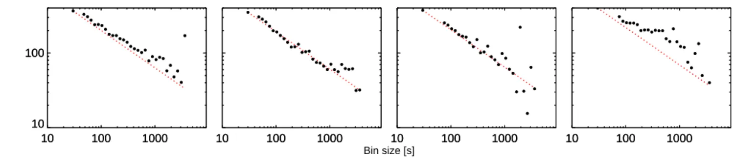
Figure 3. 2011 transit - RMS vs. binning. Black filled circles indicate the photometric residual RMS for different time bins. Each panel corresponds to each individual transit from 2011. The expected decrease in Poisson noise normalised to an individual bin (30s) precision is shown as a red dotted line.

absorbing in the IRAC 4.5µm band. Local changes in the chem-ical composition or temperature profiles of the observable atmo-sphere are unlikely to contribute such large and variable opacity on the time-scales of our observations which, nevertheless, need to be confirmed by hydrodynamical simulations of the super-Earth atmo-sphere (e.g.Zalucha et al. 2013;Carone et al. 2014;Kataria et al.

2015).

Recent studies motivate the question of whether volcanic out-gassing from the planetary surface might contribute to the observed variability. Given the high equilibrium temperature of the planet (& 2000K) the planetary lithosphere is likely weakened, if not molten, for most mineral compositions thereby leading to magma oceans and potential volcanic activity, particularly on the irradi-ated day side (Gelman et al. 2011;Elkins-Tanton 2012). Recent inferences of disintegrating exo-mercuries in close-in orbits have also used volcanic outgassing as a possible means to inject dust into the planetary atmosphere before being carried away by ther-mal winds (e.g.Rappaport et al. 2012,2014). However, whereas extremely small planets (nearly Mercury-size) subject to intense ir-radiation can undergo substantial mass loss through thermal winds, super-Earths are unlikely to undergo such mass-loss due to their significantly deeper potential wells (Perez-Becker & Chiang 2013;

Rappaport et al. 2014). Thus, ejecta from volcanic eruptions on

even the most irradiated super-Earths such as 55 Cnc e are un-likely to escape the planet and would instead display plume be-haviour characteristic to the solar system (Spencer et al. 1997,

2007;McEwen et al. 1998;S´anchez-Lavega et al. 2015). The

ex-tent and dynamics of the plumes if large enough can cause tempo-ral variations in the planetary sizes and brightness temperatures and hence in the transit and occultation depths.

Volcanic plumes may be able to explain the peak-to-trough variation in thermal emission that we observe from 55 Cnc e. As-cending plumes could raise the planetary photosphere in the 4.5 µm to lower pressures higher up in the atmosphere where the tem-peratures are lower, thereby leading to lower thermal emission as observed in Fig.11. Note that the temperature structure is governed largely by the incoming visible radiation and visible opacity in the atmosphere, whereas the infrared photosphere is governed primar-ily by the infrared opacity. Therefore, for the temperature profile to remain cooler in the upper-atmosphere the visible opacity in the atmosphere and in the rising plume would need to be weaker com-pared to the infrared opacity. The detailed hydrodynamics of a po-tential volcanic plume is outside the scope of the current work, but we can nevertheless assess its plausibility using simple arguments. The observed IRAC 4.5-µm brightness temperature (TB) of the planet varies widely between Tmin= 1273+271−348K and Tmax= 2816+358

−368K. If we assume that the Tmin and Tmax observed do indeed represent the maximum and minimum temperatures in the atmosphere, they provide a constraint on the temperature pro-file of the atmosphere. For extremely irradiated atmospheres the temperature profile approaches an isotherm in the two extremes of optical depth; i.e. a skin temperature at low optical depths and the diffusion approximation at high optical depths (see e.g.

Bin size [s] RMS [ppm] 10 100 1000 10 100 10 100 1000 10 100 10 100 1000 10 100 1000 1010 100100 10001000 1010 100100 10001000

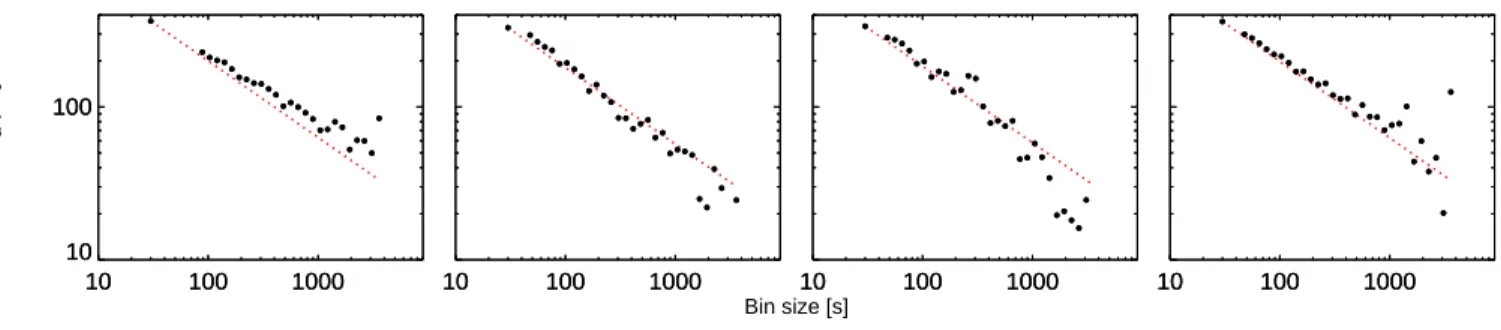
Figure 4. 2013 transit - RMS vs. binning. Black filled circles indicate the photometric residual RMS for different time bins. Each panel corresponds to each individual transit from 2013. The expected decrease in Poisson noise normalised to an individual bin (30s) precision is shown as a red dotted line.

Date obs δocc[ppm] TB[K] 2012-01-18 87±56 1767+491₋₅₉₂ 2012-01-21 44±28 1331+292−374 2012-01-23 39±25 1273+271−348 2012-01-31 82±45 1720+402−470 2013-06-15 212±46 2816+358−368 2013-06-18 201±64 2729+499₋₅₂₂ 2013-06-29 169±62 2472+493−524 2013-07-15 101±52 1894+446−507

Table 4. 55 Cnc e Spitzer occultation depths and brightness temperatures. IRAC 4.5µm occultation depths derived from the MCMC simulation detailed

in Sect.2.3.5. Brightness temperatures are computed using a stellar spectrum, as detailed in the text.

2010;Heng 2012). Therefore, TB,minand TB,maxcould represent

the two extreme isotherms. The pressures corresponding to the two limits depend on the atmospheric composition, but generally lie be-tween Pmaxof ∼ 1-100 bar and Pminof ∼10−3bar in models of irradiated atmospheres. Fig.12shows an illustrative model of aP -T profile between (-Tmin, Pmin) and (Tmax, Pmax). Note that the curvature of theT -P profile and hence the vertical location of the intermediate points are arbitrary in this toy model. The more im-portant matter is that the maximum extent of the plumes can be encompassed within ∼10 scale heights of the atmosphere, imply-ing ∼ 500 km in an H2O-rich atmosphere, and 200 or 300 km for a CO2or CO atmosphere, respectively. Such plume heights are comparable to those of the largest plumes in the solar system as discussed below (Spencer et al. 1997;McEwen et al. 1998). How-ever, depending on their aspect ratios and locations relative to the sub-stellar point multiple plumes may be required to influence the disk integrated thermal emission observed.

The chemical composition of the outgassed material is uncon-strained by our current observations and would depend on the in-terior composition of the planet. However, any candidate plume material is required to have significant opacity in the IRAC 4.5 µm bandpass. Gases such as CO2, CO, and HCN could pro-vide such opacity (e.g.Madhusudhan 2012). Using internal struc-ture models of super-Earths (Madhusudhan et al. 2012), we find that the mass and bulk radius of the planet, given by the min-imum radius observed, are consistent with an Earth-like inte-rior composition of the planet, i.e. composed of an Iron core (30% by mass) overlaid by a silicate mantle and crust. Previ-ous studies which used a larger radius of the planet required a thick water envelope (Demory et al. 2011; Gillon et al. 2012;

Winn et al. 2011) or a carbon-rich interior (Madhusudhan et al.

2012), neither of which are now required but cannot be ruled out either. However, under the assumption of an Earth-like inte-rior, which is also the case for Io, the outgassed products could comprise of gaseous CO2 and sulfur compounds (Moses et al.

2002;Schaefer & Fegley 2005) along with particulate matter

com-posed of silicates (Spencer et al. 1997;McEwen et al. 1998). The steady state composition of the atmosphere can be equally diverse

(Miguel et al. 2011;Schaefer & Fegley 2011;Hu & Seager 2014),

although the stability of a thick ambient atmosphere is uncertain

(Castan & Menou 2011;Heng & Kopparla 2012). While gaseous

products could contribute significant absorption in the IR, such as the strong CO or CO2 or HCN bands in the 4.5µm Spitzer IRAC bandpass in which our observations were made, gaseous and particulate Rayleigh scattering and particulate Mie scattering can cause substantial opacity in the visible and IR wavelengths. New high-precision high-cadence spectroscopic observations over a wide spectral range, e.g. with HST and ground-based facilities at present and with JWST in the future, will be necessary to charac-terise the chemical composition of the plume material.

On the other hand, if volcanic plumes occur along the day-night terminator of the planet they could also cause variations in the transit depths. We detect only marginal variation (1-σ) in the transit depths. Nevertheless, we briefly assess their potential impli-cations in this context. The fractional change in the transit-depth due to plumes in the vicinity of the day-night terminator is given byδ ∼ (PN

i=1ǫiH 2

i)/A0, whereA0 is the apparent area of the planet disk in quiescent phase,N is the number of plumes, Hiis the height of plume i andǫi is the aspect ratio of plume i. Con-sidering all the plumes to be of similar extent and an aspect ra-tio of unity (e.g.Spencer et al. 1997), the average plume height required to explain the variability is given by H ∼ pA0δ/N .

Time [BJD-2450000] Relative flux 5944.72 5944.80 0.9995 1.0000 1.0005 1.0010 5947.68 5947.76 5949.84 5949.92 5950.00 5958.00 5958.08

Figure 5. 2012 occultation lightcurves. Individual analyses of the Spitzer/IRAC 4.5-µm 2012 occultation data detrended and normalised following the

technique described in the text. Black filled circles are data binned per 15 minutes. The best-fit model resulting from the MCMC fit is superimposed in red for each eclipse. Time [BJD-2450000] Relative flux 6458.8 6458.9 0.9995 1.0000 1.0005 1.0010 6461.8 6461.96472.8 6472.9 6489.0 6489.1

Figure 6. 2013 occultation lightcurves. Individual analyses of the Spitzer/IRAC 4.5-µm 2013 occultation data detrended and normalised following the

technique described in the text. Black filled circles are data binned per 15 minutes. The best-fit model resulting from the MCMC fit is superimposed in red for each eclipse.

For plumes distributed over the entire terminator, the disk-averaged plume height is given byHav ∼ ∆Rp, where∆Rpis the ampli-tude of the apparent change in the planetary radius, which implies Hav∼ 1300 − 5100 km ∼ 0.1 − 0.4 Rp. On the other extreme, if only one plume is involved thenH ∼ 1 − 2.2 ×104

km ∼ 1 − 2 Rp. Thus, depending on the number of plumes, the plume height required to explain the maximum variability in transit depths can vary betweenH ∼ 0.1 - 2 Rp. The required plume heights are gen-erally larger than those found in the solar system, though not im-plausible. The highest plumes in the solar system are typically seen in bodies with low gravities, such as Io and Mars. The highest vol-canic plumes on Jupiter’s moon Io (radius,RIo = 1821 km) have heights of ∼ 300-500 km or 0.16-0.27 RIo (Spencer et al. 1997;

McEwen et al. 1998). Recently, the highest plume on Mars was

re-ported at the day-night terminator with a height of ∼250 km (0.07 RMars) and a width of 500-1000 km, i.e with aspect ratio over 2:1

(S´anchez-Lavega et al. 2015). The source of the Martian plume is

currently unknown though apparently non-volcanic.

The required plume heights are in principle attainable given the planet’s orbital parameters. The Hill radius of the planet is given byRHill= a(Mp/3Ms)1/3wherea is the orbital separation and MpandMsare the masses of the planet and star, respectively. The required plume heights are well within the Hill radius of 55 Cnc e,RHill ∼ 3.5Rp, implying that the ejecta is unlikely to escape the system and will fall back to the surface. Furthermore,

follow-ingRappaport et al.(2012), the sound speed (vs) at the surface of

the planet is ∼1 km/s which is significantly lower than the escape

velocity (vesc) of 24 km/s at the planetary surface thereby prevent-ing a Parker-type wind to carry the ejecta beyond the Hill sphere. On the other hand, the velocity of the ejecta required to sustain Hav∼ 1300 − 5100 km is between 8-17 km/s, which is below the escape velocity of the planet (24 km/s) and is significantly lower than the maximal ejection velocities of ∼300 km/s observed on Io. Alternately, the data may also be potentially explained by the presence of an azimuthally inhomogeneous circumstellar torus made of ions and charged dust particles similar to Io (Kr¨uger et al. 2003) that could contribute a variable gray opacity along the line-of-sight through diffusion of stellar light. While CO gas in the torus could provide the required opacity in the 4.5µm bandpass, the grey behaviour of dust could provide the same opacity both in the visible and infrared. Io’s cold torus rotates with the orbital period of Jupiter (Belcher 1987). Assuming the same scenario holds for 55 Cnc e would mean that the torus rotates with the same period as the host star (∼42 days), which would cause a modulation of the transit and occultation depths over similar timescales. For such a circumstellar torus, the optical depth of the time-varying torus segment occulting the stellar disk governs the observed stellar ra-dius and hence the transit depth; for the same planetary rara-dius, a denser segment causes a deeper transit compared to a lighter seg-ment. Thus, a denser segment gradually coming into view could cause the observed increase in transit depth. Similarly for the oc-cultation depth, increasing the optical depth of the segment could result in a decrease in the occultation depth. Volcanism could pro-vide a source for the torus’ material akin to Io (Kr¨uger et al. 2003).

Bin size [s] RMS [ppm] 10 100 1000 10 100 10 100 1000 10 100 10 100 1000 10 100 1000 1010 100100 10001000 1010 100100 10001000

Figure 7. 2012 occultation - RMS vs. binning. Black filled circles indicate the photometric residual RMS for different time bins. Each panel corresponds to each individual occultation from 2012. The expected decrease in Poisson noise normalised to an individual bin (30s) precision is shown as a red dotted line.

Bin size [s] RMS [ppm] 10 100 1000 10 100 10 100 1000 10 100 10 100 1000 10 100 1000 1010 100100 10001000 1010 100100 10001000

Figure 8. 2013 occultation - RMS vs. binning. Black filled circles indicate the photometric residual RMS for different time bins. Each panel corresponds to each individual occultation from 2013. The expected decrease in Poisson noise normalised to an individual bin (30s) precision is shown as a red dotted line.

Analysis # Occ. depth [ppm] BIC χ2 _{RMS/15 min [ppm]}

T1 47±21 2938 2596.1 64 T2 156±37 3583 3068.5 96 T3 101±55 2983.4 2592.9 64 61±37 94±33 152±46 T4 220±64 3618.6 3056.1 93 55+56−38 132+120−84 217+55−61

Table 5. 55 Cnc baseline model test. The table indicates the results of the different baseline model tests conducted to investigate the discrepancy with the results of Demory et al. 2012 (D12). Analysis T1 shows the fit results from the present analysis, using the same data from D12 and the baseline model presented in this study. T2 uses the same photometry but with the baseline models from D12. T3 and T4 are similar to T1 and T2 respectively but allow each occultation depth to be fit independently.

Model BIC RMS/15 min [ppm] Occ. depth [ppm]

p(x,y,wx,wy) 2905 64 97±22

p(x,y,t,r) 3585 118 63±34

Table 6. 55 Cnc e occultation injection test. The table indicate how well our fake 100-ppm deep occultation is recovered by the baseline model used in the present studyp(x,y,wx,wy) and by the baseline model used in D12p(x,y,t,r). x, y are the PSF positions, t is time, r is the logarithmic ramp and wx,wyare the width of the PSF along thex and y axes respectively.

0.30 0.32 0.34 0.36 0.38 0.40 0.42 0.44 Time since transit [days]

0.9996 0.9998 1.0000 1.0002 1.0004 Relative flux 0.30 0.32 0.34 0.36 0.38 0.40 0.42 0.44 Time since transit [days]

0.9996 0.9998 1.0000 1.0002 1.0004 Relative flux

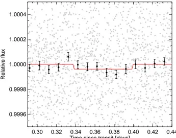
Figure 9. 55 Cnc e Spitzer/IRAC 4.5µm 2012 vs. 2013 occultations. The top and bottom lightcurves are the combined occultations for 2012 and 2013

respectively. Each season results from co-adding four occultations. Data are detrended from instrumental systematics and normalised following the technique described in the text. Black datapoints are binned per 15 minutes. Best-fit occultation models are superimposed in red.

Future observational and theoretical studies are needed to explore this alternative. Constraining the nature of the material surround-ing 55 Cnc e will be a direct probe of the planet surface composi-tion and may also constrain the formacomposi-tion pathway of hundreds of similar planets that have been found so far.

ACKNOWLEDGMENTS

We thank Drake Deming for having performed an independent check of the occultation variability and depths in the Spitzer

4.5-µm data using his pixel-level decorrelation technique. B.-O.D. thanks Kevin Heng and Caroline Dorn for discussions. We thank the Spitzer Science Center staff for their assistance in the planning and executing of these observations. We thank the anonymous ref-eree for an helpful review. This work is based in part on obser-vations made with the Spitzer Space Telescope, which is operated by the Jet Propulsion Laboratory, California Institute of Technol-ogy under a contract with NASA. Support for this work was pro-vided by NASA through an award issued by JPL/Caltech. M.G. is Research Associate at the Belgian Funds for Scientific Research

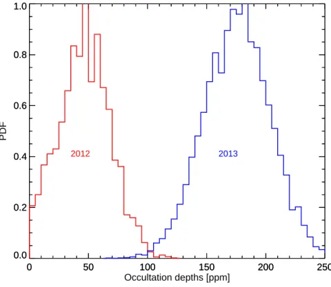
0 50 100 150 200 250 0.0 0.2 0.4 0.6 0.8 1.0 0 50 100 150 200 250 Occultation depths [ppm] 0.0 0.2 0.4 0.6 0.8 1.0 PDF 2012 2013

Figure 10. 55 Cnc e average occultation depthsδoccin 2012 and 2013. Posterior probability distribution functions for the 2012 (red) and 2013 (blue) mean occultation depths. Both histograms indicate the entire credible region constrained by the Spitzer data using an MCMC fit.

(F.R.S-FNRS). This research made use of the IDL Astronomical Library and the IDL-Coyote Graphics Library.

REFERENCES

Agol E., Cowan N. B., Knutson H. A., Deming D., Steffen J. H., Henry G. W., Charbonneau D., 2010, ApJ, 721, 1861

Ballard S., Charbonneau D., Deming D., Knutson H. A., Christiansen J. L., Holman M. J., Fabrycky D., Seager S., A’Hearn M. F., 2010, PASP, 122, 1341

Barnes R., Raymond S. N., Greenberg R., Jackson B., Kaib N. A., 2010, ApJ, 709, L95

Beerer I. M., Knutson H. A., Burrows A., Fortney J. J., Agol E., Charbon-neau D., Cowan N. B., Deming D., Desert J.-M., Langton J., Laughlin G., Lewis N. K., Showman A. P., 2011, ApJ, 727, 23

Belcher J. W., 1987, Science, 238, 170

Bochinski J. J., Haswell C. A., Marsh T. R., Dhillon V. S., Littlefair S. P., 2015, ArXiv e-prints

Bolmont E., Selsis F., Raymond S. N., Leconte J., Hersant F., Maurin A.-S., Pericaud J., 2013, A&A, 556, A17

Brogi M., Keller C. U., de Juan Ovelar M., Kenworthy M. A., de Kok R. J., Min M., Snellen I. A. G., 2012, A&A, 545, L5

Carone L., Keppens R., Decin L., 2014, MNRAS, 445, 930 Castan T., Menou K., 2011, ApJ, 743, L36

Charbonneau D., Allen L. E., Megeath S. T., Torres G., Alonso R., Brown T. M., Gilliland R. L., Latham D. W., Mandushev G., O’Donovan F. T., Sozzetti A., 2005, ApJ, 626, 523

Claret A., Bloemen S., 2011, A&A, 529, 75

Croll B., Rappaport S., DeVore J., Gilliland R. L., Crepp J. R., Howard

A. W., Star K. M., Chiang E., Levine A. M., Jenkins J. M., Albert L., Bonomo A. S., Fortney J. J., Isaacson H., 2014, ApJ, 786, 100 Crossfield I. J. M., 2012, A&A, 545, A97

Deming D., Knutson H., Agol E., Desert J.-M., Burrows A., Fortney J. J., Charbonneau D., Cowan N. B., Laughlin G., Langton J., Showman A. P., Lewis N. K., 2011, ApJ, 726, 95

Deming D., Knutson H., Kammer J., Fulton B. J., Ingalls J., Carey S., Burrows A., Fortney J. J., Todorov K., Agol E., Cowan N., Desert J.-M., Fraine J., Langton J., Morley C., Showman A. P., 2014, ArXiv e-prints Demory B.-O., Gillon M., Deming D., Valencia D., Seager S., Benneke B.,

Lovis C., Cubillos P., Harrington J., Stevenson K. B., Mayor M., Pepe F., Queloz D., S´egransan D., Udry S., 2011, A&A, 533, 114

Demory B.-O., Gillon M., Seager S., Benneke B., Deming D., Jackson B., 2012, ApJ, 751, L28

Eastman J., Siverd R., Gaudi B. S., 2010, PASP, 122, 935

Elkins-Tanton L. T., 2012, Annual Review of Earth and Planetary Sci-ences, 40, 113

Fazio G. G., Hora J. L., Allen L. E., Ashby M. L. N., Barmby P., Deutsch L. K., Huang 2004, ApJS, 154, 10

Fischer D. A., Marcy G. W., Butler R. P., Vogt S. S., Laughlin G., Henry G. W., Abouav D., Peek K. M. G., Wright J. T., Johnson J. A., McCarthy C., Isaacson H., 2008, ApJ, 675, 790

Gelman Rubin 1992, Statistical Science, 7, 457

Gelman S. E., Elkins-Tanton L. T., Seager S., 2011, ApJ, 735, 72 Gillon M., Demory B.-O., Benneke B., Valencia D., Deming D., Seager S.,

Lovis C., Mayor M., Pepe F., Queloz D., S´egransan D., Udry S., 2012, A&A, 539, A28

Gillon M., Triaud A. H. M. J., Fortney J. J., Demory B.-O., Jehin E., Lendl M., Magain P., Kabath P., Queloz D., Alonso R., Anderson D. R., Collier Cameron A., Fumel A., Hebb L., Hellier C., Lanotte A., Maxted P. F. L., Mowlavi N., Smalley B., 2012, A&A, 542, A4

Time [BJD-2,450,000]

Figure 11. 55 Cnc e Spitzer/IRAC 4.5µm occultation and transit depths. Top and bottom panels indicate the occultation and transit depths with time. Left

panels are for 2011, middle panels for 2012 and right panels for 2013. The grey solid horizontal lines indicate the mean depths and the dotted lines the 1-σ

credible intervals.

Guillot T., 2010, A&A, 520, A27 Heng K., 2012, ApJ, 748, L17

Heng K., Kopparla P., 2012, ApJ, 754, 60 Hu R., Seager S., 2014, ApJ, 784, 63

Ingalls J. G., Krick J. E., Carey S. J., Laine S., Surace J. A., Glaccum W. J., Grillmair C. C., Lowrance P. J., 2012, in Society of Photo-Optical Instrumentation Engineers (SPIE) Conference Series Vol. 8442 of Soci-ety of Photo-Optical Instrumentation Engineers (SPIE) Conference Se-ries, Intra-pixel gain variations and high-precision photometry with the Infrared Array Camera (IRAC)

Jackson B., Barnes R., Greenberg R., 2008, MNRAS, 391, 237

Kataria T., Showman A. P., Fortney J. J., Stevenson K. B., Line M. R., Kreidberg L., Bean J. L., D´esert J.-M., 2015, ApJ, 801, 86

Knutson H. A., Dragomir D., Kreidberg L., Kempton E. M.-R., McCul-lough P. R., Fortney J. J., Bean J. L., Gillon M., Homeier D., Howard A. W., 2014, ApJ, 794, 155

Kreidberg L., Bean J. L., D´esert J.-M., Benneke B., Deming D., Stevenson K. B., Seager S., Berta-Thompson Z., Seifahrt A., Homeier D., 2014, Nat, 505, 69

Kr¨uger H., Geissler P., Hor´anyi M., Graps A. L., Kempf S., Srama R., Moragas-Klostermeyer G., Moissl R., Johnson T. V., Gr¨un E., 2003, Geo-phys. Res. Lett., 30, 2101

Lanotte A. A., Gillon M., Demory B.-O., Fortney J. J., Astudillo N., Bon-fils X., Magain P., Delfosse X., Forveille T., Lovis C., Mayor M., Neves V., Pepe F., Queloz D., Santos N., Udry S., 2014, A&A, 572, A73 Lewis N. K., Knutson H. A., Showman A. P., Cowan N. B., Laughlin 2013,

ApJ, 766, 95

Madhusudhan N., 2012, ApJ, 758, 36

Madhusudhan N., Lee K. K. M., Mousis O., 2012, ApJ, 759, L40 Madhusudhan N., Redfield S., 2015, International Journal of

Astrobiol-ogy, 14, 177

Madhusudhan N., Seager S., 2009, ApJ, 707, 24 Mandel K., Agol E., 2002, ApJ, 580, L171

McEwen A. S., Keszthelyi L., Geissler P., Simonelli D. P., Carr M. H., Johnson T. V., Klaasen K. P., Breneman H. H., Jones T. J., Kaufman J. M., Magee K. P., Senske D. A., Belton M. J. S., Schubert G., 1998, Icarus, 135, 181

Miguel Y., Kaltenegger L., Fegley B., Schaefer L., 2011, ApJ, 742, L19 Moses J. I., Zolotov M. Y., Fegley B., 2002, Icarus, 156, 76

Nelson B. E., Ford E. B., Wright J. T., Fischer D. A., von Braun K., Howard A. W., Payne M. J., Dindar S., 2014, MNRAS

Owen J. E., Wu Y., 2013, ApJ, 775, 105

Perez-Becker D., Chiang E., 2013, MNRAS, 433, 2294

Pont F., Knutson H., Gilliland R. L., Moutou C., Charbonneau D., 2008, Monthly Notices of the Royal Astronomical Society, 385, 109 Pont F., Zucker S., Queloz D., 2006, Monthly Notices of the Royal

Astro-nomical Society, 373, 231

Rappaport S., Barclay T., DeVore J., Rowe J., Sanchis-Ojeda R., Still M., 2014, ApJ, 784, 40

Rappaport S., Levine A., Chiang E., El Mellah I., Jenkins J., Kalomeni B., Kite E. S., Kotson M., Nelson L., Rousseau-Nepton L., Tran K., 2012, ApJ, 752, 1

Figure 12. 55 Cnc e arbitrary pressure-temperature profile. Schematic representation of the observed brightness temperatures in the IRAC 4.5µm relative

to an illustrative temperature profile of the dayside atmosphere of 55 Cnc e. The data show the measured brightness temperatures along with their uncertainties. The solid gray curve shows a schematic temperature profile as discussed in Section3.

S´anchez-Lavega A., Mu˜noz A. G., Garc´ıa-Melendo E., P´erez-Hoyos S., G ´omez-Forrellad 2015, Nat, 518, 525

Sanchis-Ojeda R., Rappaport S., Winn J. N., Kotson M. C., Levine A., El Mellah I., 2014, ApJ, 787, 47

Schaefer L., Fegley B., 2009, ApJ, 703, L113 Schaefer L., Fegley Jr. B., 2005, ApJ, 618, 1079 Schaefer L., Fegley Jr. B., 2011, ApJ, 729, 6 Schwarz G., 1978, The Annals of Statistics, 6, 461

Sing D. K., Pont F., Aigrain S., Charbonneau D., D´esert J.-M., Gibson N., Gilliland R., Hayek W., Henry G., Knutson H., Lecavelier Des Etangs A., Mazeh T., Shporer A., 2011, MNRAS, 416, 1443

Spencer J. R., Sartoretti P., Ballester G. E., McEwen A. S., Clarke J. T., McGrath M. A., 1997, Geophys. Res. Lett., 24, 2471

Spencer J. R., Stern S. A., Cheng A. F., Weaver H. A., Reuter D. C., Retherford K., Lunsford A., Moore J. M., Abramov O., Lopes R. M. C., Perry J. E., Kamp L., Showalter M., Jessup K. L., Marchis F., Schenk P. M., Dumas C., 2007, Science, 318, 240

Spiegel D. S., Burrows A., 2010, ApJ, 722, 871

Stevenson K. B., Harrington J., Fortney J. J., Loredo T. J., Hardy R. A., Nymeyer S., Bowman W. C., Cubillos P., Bowman M. O., Hardin M., 2012, ApJ, 754, 136

von Braun K., Boyajian T. S., ten Brummelaar T. A., Kane S. R., van Belle 2011, ApJ, 740, 49

Werner M. W., Roellig T. L., Low F. J., Rieke G. H., Rieke M., 2004, ApJS, 154, 1

Winn J. N., Matthews J. M., Dawson R. I., Fabrycky D., Holman M. J., Kallinger T., Kuschnig R., Sasselov D., Dragomir D., Guenther D. B., Moffat A. F. J., Rowe J. F., Rucinski S., Weiss W. W., 2011, ApJ, 737, L18

Zalucha A. M., Michaels T. I., Madhusudhan N., 2013, Icarus, 226, 1743

This paper has been typeset from a TEX/ LA_{TEX file prepared by the} author.