IMPROVEMENT OF SUBSONIC WALL CORRECTIONS
IN AN INDUSTRIAL WIND TUNNEL
by
Alvaro TOLEDANO ESCALONA
THESIS PRESENTED TO ÉCOLE DE TECHNOLOGIE SUPÉRIEURE
IN PARTIAL FULFILLMENT FOR THE DEGREE OF
DOCTOR OF PHILOSOPHY
Ph.D.
MONTRÉAL, OCTOBER 22, 2019
ÉCOLE DE TECHNOLOGIE SUPÉRIEURE
UNIVERSITÉ DU QUÉBEC
Cette licence Creative Commons signifie qu’il est permis de diffuser, d’imprimer ou de sauvegarder sur un autre support une partie ou la totalité de cette œuvre à condition de mentionner l’auteur, que ces utilisations soient faites à des fins non commerciales et que le contenu de l’œuvre n’ait pas été modifié.
BOARD OF EXAMINERS
THIS THESIS HAS BEEN EVALUATED
BY THE FOLLOWING BOARD OF EXAMINERS:
Mr. Julien Weiss, Thesis Supervisor
Department of Mechanical Engineering at École de technologie supérieure
Mr. Simon Joncas, Chair, Board of Examiners
Department of Systems Engineering at École de technologie supérieure
Mr. Patrice Seers, Member of the Jury
Department of Mechanical Engineering at École de technologie supérieure
Mr. Norbert Ulbrich, External Evaluator NASA Ames Research Center
Mr. Marc Langlois, External Evaluator Bombardier Aerospace
Mr. Cabot Broughton, External Evaluator National Research Council of Canada
THIS DISSERTATION WAS PRESENTED AND DEFENDED IN THE PRESENCE OF A BOARD OF EXAMINERS AND PUBLIC
ON AUGUST 27 2019
ACKNOWLEDGEMENTS
A sincere thank you to my Ph.D. advisor, Professor Julien Weiss, for the opportunity provided to carry out this research project and his assistance over these years.
I would like to thank the staff at the Uplands Campus of the National Research Council, with special mention to Cabot Broughton, an undeniable source of advice and expertise throughout my journey in the world of wind-tunnel testing.
To all members of the jury, because I profoundly respect you and your work and I am honored to present you with the fruit of my research.
To my parents, my brothers and my sister; because despite the enormous distance between us you have believed in me and supported me when I decided to take up this beautiful but incredibly tough endeavor .
Finally, I would like to acknowledge the support of Bombardier Inc., the Natural Sciences and Engineering Research Council of Canada and the National Research Council’s Aeronautical Product Development Technologies program.
Improvement of subsonic wall corrections in an industrial wind tunnel Alvaro TOLEDANO ESCALONA
ABSTRACT
The National Research Council 5ft Trisonic Wind Tunnel enables testing of half-span models at a high Reynolds number cost effectively, however there is the possibility of experiencing relatively larger wall-interference effects compared to full span tests. Subsonic wall-interference effects due to the partially open boundaries at the NRC 5ft wind tunnel are corrected by the “one-variable” method, resulting in corrections in Mach number and angle of attack for the measured quantities. This dissertation introduces the need for adequately correcting for wall interference in subsonic half-model wind-tunnel testing in both pre-stall and post-stall conditions. The one-variable method is described and several aspects that require validation and improvement in this method are pointed out based on specific experimental and numerical results obtained for different test articles.
An initial assessment of the influence of the different possible tunnel configurations and computational parameters is defined based on experimental data from a test performed on a scaled model of the Bombardier Global 6000 business jet. This initial study unveils some of the weaknesses of the one-variable method. While this method provides accurate wall corrections during tests in pre-stall conditions; it is unable to generate reliable corrections in stall. Partially, this is due to the development of flow separation on a model tested at subsonic flow conditions reaching stall, not currently accounted for by the potential theory model representation used by the wall-correction methodology at the NRC 5ft TWT. Possible improvements to this singularity representation, paramount to the one-variable method, are then investigated. This revision of the model representation is based on high fidelity free-air CFD solutions for the NASA Common Research Model, validated by experimental data sets obtained from a semispan version of the CRM tested at the NRC 5ft Trisonic Wind Tunnel. The improved potential representation is tested on solid-wall experimental wind-tunnel data to present more reliable behavior of the wall-interference correction estimates when substantial wing stalling is encountered.
Keywords: wind tunnel, wall interference, wall correction, half-span, ground testing, subsonic flow, computational fluid dynamics.
Améliorations des corrections de parois en écoulement subsonique dans une soufflerie industrielle
Alvaro TOLEDANO ESCALONA RÉSUMÉ
La soufflerie trisonique de 5 pieds du Conseil National de Recherches du Canada permet de réaliser des essais demi-maquette à un nombre de Reynolds élevé de façon efficace. En revanche, on peut s’attendre à des effets d'interférence des murs relativement plus importants que ceux rencontrés lors des essais avec des maquettes à pleine envergure. Les effets d'interférence de paroi subsoniques dus aux limites partiellement ouvertes de la soufflerie de 5 pieds du CNRC sont corrigés par la méthode “one-variable”. Cette méthode fournit des corrections pour le nombre de Mach et de l'angle d'attaque mesurés. Dans ces travaux est introduit le besoin de corriger de manière appropriée l’interférence des parois dans les essais demi-maquette en écoulement subsonique, avant et après le décrochage.
Une évaluation initiale de l'influence des différentes configurations de la soufflerie et des paramètres de calcul possibles, est définie à partir de données expérimentales provenant d'un essai effectué sur un modèle à échelle réduite du jet d'affaires Bombardier Global 6000. Cette étude initiale met en lumière les limitations de la méthode one-variable. Bien qu’elle fournisse des corrections de paroi précises pendant les essais dans des conditions de pré-décrochage, cette méthode ne permet pas de générer des corrections fiables en conditions de décrochage. Cela est dû en partie au fait que le modèle utilisée par la méthode de correction des murs, basé dans la théorie d’écoulement potentiel, ne prends pas actuellement en compte ces conditions. Des améliorations de cette représentation potentielle du modèle, essentielle à la méthode one-variable, sont étudiées par la suite. Cette révision de la représentation du modèle est basée sur des résultats CFD obtenus pour le NASA Common Research Model, validés ensuite par des données expérimentales obtenues à partir d'une version demi-maquette du CRM testée à la soufflerie trisonique de 5 pieds du CNRC. La nouvelle représentation potentielle proposée, est finalement testée sur des données expérimentales de soufflerie à paroi solide, ce qui permet d’obtenir des corrections de paroi plus fiables lorsque le décrochage de l'aile est significatif.
Mots-clés : soufflerie, interférence parois, corrections parois, demi-maquette, essais au sol, écoulement subsonique, mécanique des fluides numérique.
TABLE OF CONTENTS
Page
INTRODUCTION ...1
0.1 History and background ...3
0.2 Scope and approach ...5
CHAPTER 1 LITERATURE REVIEW AND STATE OF THE ART ...7
1.1 Main factors of aerodynamic interference in wind-tunnel testing ...9
1.1.1 Flow speed ... 9
1.1.2 Wind-tunnel models ... 14
1.1.3 Wind-tunnel design ... 15
1.1.4 Nature of the wind-tunnel test ... 19
1.2 Wind-tunnel wall-interference correction ...20
1.2.1 Classification of wall corrections ... 21
1.2.2 Wall-correction calculation techniques ... 24
1.2.3 Wall-correction methods ... 28
1.3 The one-variable method at the NRC 5ft TWT ...36
1.4 Problem statement ...42
CHAPTER 2 OBJECTIVES ...45
2.1 Main goal - Improve wall corrections in stall conditions ...45
2.2 Secondary objectives ...45
CHAPTER 3 METHODOLOGY ...47
3.1 Development of an offline test bench for the one-variable method ...47
3.2 Geometries considered for the investigations at the NRC 5ft TWT ...49
3.2.1 Bombardier Global 6000 ... 49
3.2.2 NRC Symmetrical Calibration Wing ... 50
3.2.3 NASA Common Research Model ... 54
3.3 Study of the NASA Common Research Model (CRM) at NRC TWT ...57
3.3.1 NASA CRM experimental test campaign ... 58
3.3.2 NASA CRM numerical simulations ... 59
3.4 The use of CFD to improve and validate wall corrections ...66
CHAPTER 4 RESULTS ...69
4.1 Parametric study on semispan models tested at the NRC 5ft TWT ...69
4.2 CFD-based Validation of the Complete Wall Correction Algorithm ...74
4.3 Improvement of the current non-pitching Rankine body fuselage representation ...76
4.4 Improvement of the current wing representation ...84
4.5 Overall improvement to Wall Corrections ...97
4.6 CFD-based Wall-Correction Data Set ...98
CONCLUSIONS AND PERSPECTIVES ...103 REFERENCES……. ...107
LIST OF TABLES
Page
Table 1.1 Classification of wall corrections. ...23
Table 1.2 Keller Wall Boundary Conditions coefficients. ...33
Table 1.3 Semispan Global 6000 test campaign matrix. ...42
Table 3.1 NRC calibration wing (Calwing) geometry specifications. ...50
Table 3.2 Test configuration during NRC TWT run 56303 for the NACA 0012 “calwing”. ...52
Table 3.3 Semispan CRM geometry specifications. ...55
Table 3.4 Normalized spanwise section location η of the pressure port rows on the semispan CRM wing. ...56
Table 3.5 Semispan CRM test campaign matrix. ...58
LIST OF FIGURES
Page
Figure 0.1 Stages of the aircraft design process, from concept to
manufacturing. ...1 Figure 1.1 Different approaches to obtain high Reynolds number by adjusting
wind-tunnel testing parameters ...8 Figure 1.2 Wall interference described as the difference between the
wind-tunnel and free-air flow fields. ...9 Figure 1.3 Elementary singularities of the Laplace equation in potential flow
models. From: Krynytzky and Ewald in AGARDograph 336
(1998). ...11 Figure 1.4 Example of a potential theory representation for an aircraft
wind-tunnel model. From: Iyer and Everhart (2001). ...12 Figure 1.5 Sketch of a full-span model (left) and a semispan model (right) of
an aircraft in the same test section. Notice the higher model
span-to-tunnel width ratio for the semispan case. ...14 Figure 1.6 Overview of the NRC 5ft Trisonic Wind Tunnel. ...16 Figure 1.7 Detail view of the wall perforations in the NRC 5ft wind-tunnel
test section. ...18 Figure 1.8 Layout of the reflection-plate and pressure rails in the NRC 5ft
wind-tunnel test section. ...19 Figure 1.9 Contour plot showing the variation of the angle-of-attack over a
tunnel model to illustrate the concept of first and higher order
corrections. ...23 Figure 1.10 Vortex near a solid boundary and image vortex placed to guarantee
the no flow through condition. From: Kuethe and Chow (1986). ...25 Figure 1.11 Illustration of the method of images: Image system for a wing in a
closed rectangular tunnel. From: Rae and Pope (1984). ...26 Figure 1.12 Example of a discretization of the geometry of a three-dimensional
body using a panel representation with constant-strength surface
Figure 1.13 NASA Ames 12ft PWT test section interior and paneling. From:
Ulbrich (1998). ...32
Figure 1.14 Real-time wall interference calculation at NASA Ames 11ft TWT. From: Ulbrich et al. (2003). ...34
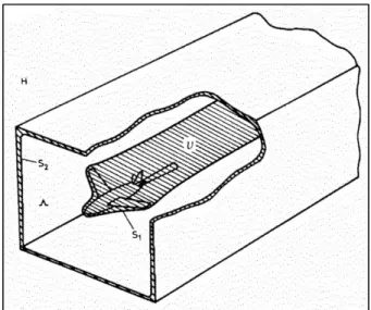
Figure 1.15 Region and bounding surfaces for application of Green’s theorem. From: Ashill et al. (1982). ...35
Figure 1.16 Distribution of pressure rows in the RAE 13ft x 9ft Low-Speed Wind Tunnel From: Ashill et al. (1988). ...36
Figure 1.17 NRC 5ft TWT test section and mirror image respect to reflection plane. ...38
Figure 1.18 Panel distribution on boundary test surface. ...39
Figure 1.19 Interference velocity interpolation sequence. ...40
Figure 1.20 Angle-of-attack correction for the Global 6000 solid-wall data set. ...43
Figure 3.1 Contour maps including Mach number and angle of attack corrections. The red dot indicates the location of the model’s reference point in the wind tunnel. ...48
Figure 3.2 Semispan Bombardier Global 6000 model. ...49
Figure 3.3 Semispan NRC calibration wing (Calwing) model. ...51
Figure 3.4 Assembly of semispan calibration wing (Calwing) at NRC TWT. ...52
Figure 3.5 Experimentally measured aerodynamic coefficients for the symmetrical calibration wing tested at the NRC TWT with a solid-wall test boundary at M=0.25 and Re=3.97x10⁶ ...53
Figure 3.6 NRC experimental wing pressure distributions at α=15º measured on the symmetrical calibration wing tested at the NRC TWT (run 56303). ...54
Figure 3.7 NRC experimental wing pressure distributions at α=20º measured on the symmetrical calibration wing tested at the NRC TWT (run 56303). ...54
Figure 3.8 Location of the nine rows of wing pressure taps at the 2.7% scale semispan NASA CRM. ...56
Figure 3.10 Coarse (left), medium (middle) and fine (right) CRM surface
meshes. ...60 Figure 3.11 Measured model loads at α=5.02º compared to those predicted by
CFD at α=5º using the three meshes considered versus the number
of grid points N to the power of -2/3. ...61 Figure 3.12 Measured model loads at α=12.32º compared to those predicted by
CFD at α=12.5º using the three meshes considered versus the
number of grid points N to the power of -2/3. ...61 Figure 3.13 CFD predicted aerodynamic coefficients for the CRM WB
half-model (red-filled CFD data points indicate flow separation is significant) compared to ventilated-wall NRC experimental results
(run 56307)...62 Figure 3.14 CFD predicted wing pressure distributions at α=0º compared to
NRC experimental ventilated-wall results (run 56307) at α=0.08º...63 Figure 3.15 CFD-predicted evolution of the flow separation over the CRM
wing. The x-component of the skin friction coefficient vector is
used to indicate flow separation on the suction side of the wing. ...64 Figure 3.16 CFD predicted wing pressure distributions at α=11.25º compared
to NRC experimental ventilated-wall results (run 56307) at
α=11.29º. ...65 Figure 3.17 CFD predicted wing pressure distributions at α=14º compared to
NRC experimental ventilated-wall results (run 56307) at α=13.93º...65 Figure 3.18 Theoretical “zero” wall interference described as the difference
between CFD-predicted and potential theory free-air flow fields. ...67 Figure 3.19 Mach and angle-of-attack “zero-correction” uncertainty budget
based on AGARDograph 184. ...68 Figure 4.1 Computational boundary for panel method. From: Mokry et al.
(1987). ...70 Figure 4.2 Results from the computational boundary surface parametric study
using solid-wall experimental data from a test performed on the
Bombardier Global 6000 model. ...71 Figure 4.3 Results from the reference pressure re-adjustment using solid-wall
experimental data from a test performed on the Bombardier Global
Figure 4.4 Original (top) and extended (bottom) versions of the NRC TWT
reflection plate. ...73 Figure 4.5 Results from the study of the influence of the reflection plane
extension using solid-wall experimental data from a test performed
on the Bombardier Global 6000 model. ...74 Figure 4.6 Validation of the one-variable method using free-air CFD results
as input. ...75 Figure 4.7 Rankine body fuselage representation over sketch of the CRM
fuselage relative to the NRC 5ft TWT boundary location. ...77 Figure 4.8 Pressure signature at the Top North (TN) rail location comparing
(a) the Rankine body fuselage representation to (b) a CFD
simulation of the actual 2.7% scale NASA CRM fuselage. ...78 Figure 4.9 Error band for Mach number and angle of attack corrections
computed using the one-variable method applying the original
fuselage representation of the CRM. ...79 Figure 4.10 Singularity distribution in the updated fuselage representation over
sketch of the CRM fuselage relative to the NRC 5ft TWT
boundary location...81 Figure 4.11 Pressure signature at the Top North (TN) rail comparing (a) the
updated fuselage representation to (b) a CFD simulation of the
actual 2.7% scale NASA CRM fuselage. ...82 Figure 4.12 CFD validation of the n=22 sources-sinks and n=22 doublets
fuselage representation for α=0°. ...82 Figure 4.13 CFD validation of the n=22 sources-sinks and n=22 doublets
fuselage representation for α=10°. ...83 Figure 4.14 CFD validation of the n=22 sources-sinks and n=22 doublets
fuselage representation for α=20°. ...83 Figure 4.15 Error band for Mach number and angle of attack corrections
computed using the one-variable method applying the updated
fuselage representation of the CRM. ...84 Figure 4.16 Sketch of the singularity distribution employed to represent the
Figure 4.17 Comparison between the farfield pressure signature estimated by the potential-theory representation of the CRM and that predicted
by CFD at α=0°, CL=0.195.. ...87
Figure 4.18 Comparison between the farfield pressure signature estimated by the potential-theory representation of the CRM and that predicted
by CFD at α=14°, CL=1.033.. ...87
Figure 4.19 Error band for Mach number and angle of attack corrections computed using the one-variable method applying the original
wing representation of the CRM WB. ...88 Figure 4.20 CFD predicted separation bubble at the CRM wing at α=11.25º. ...89 Figure 4.21 CFD predicted separation bubble at the CRM wing at α=14º. ...90 Figure 4.22 Qualitative estimation of the separation bubble size over the CRM
WB at α=14º. ...90 Figure 4.23 Sketch of the singularity distribution employed to represent the
model’s wing, including a doublet distribution to represent the
separation bubble volume effects. ...91 Figure 4.24 CFD predicted separation bubble at CRM wing station η=0.950 at
α=14º. The streamlines illustrate the recirculating flow region in
the bubble. ...92 Figure 4.25 Error band for Mach number and angle of attack corrections
computed using the one-variable method including the separation
bubble volume on the wing representation of the CRM WB. ...92 Figure 4.26 Sketch of the singularity distribution employed to represent the
model’s wing, including the redistribution of the horseshoe vortices to account for flow separation at the outboard region of
the wing. ...94 Figure 4.27 Error band for Mach number and angle of attack corrections
computed using the one-variable method including the skin friction estimated effective span on the wing representation of the CRM
WB. ...94 Figure 4.28 Comparison between the farfield pressure signature estimated by
the potential-theory representation of the CRM considering the lift vortices redistribution (based on skin friction data from CFD
Figure 4.29 Error band for Mach number and angle of attack corrections computed using the one-variable method including the wing pressure tap estimated effective span on the wing representation of
the CRM WB. ...96 Figure 4.30 Error band for Mach number and angle of attack corrections
computed using the one-variable method including the balance data estimated effective span on the wing representation of the
CRM WB. ...97 Figure 4.31 Comparison between Mach number and angle of attack corrections
computed using the one-variable method for the half-model CRM WB solid-wall test, using the original and updated potential theory
model representations. ...98 Figure 4.32 CFD predicted aerodynamic coefficients for the CRM WB
half-model (red-filled CFD data points indicate flow separation is significant) compared to solid-wall NRC experimental results from
run 56306. ...99 Figure 4.33 Mach number and angle of attack corrections computed using the
one-variable method for the half-model CRM WB solid-wall test,
based on the validated free-air CFD results. ...100 Figure 4.34 Additional Mach number corrections computed using the
one-variable method to rectify the supersonic bubble effects over
LIST OF ABBREVIATIONS
AGARD Advisory Group for Aerospace Research and Development AIAA American Institute of Aeronautics and Astronautics
CASI Canadian Aeronautics and Space Institute CFD Computational Fluid Dynamics
CRM (NASA) Common Research Model
DFS Design and Fabrication Services (of NRC) DND Department of National Defense (Canada) ESDU Engineering Sciences Data Unit
ESP Electronically Scanned Pressure ETW European Transonic Windtunnel JAXA Japan Aerospace Exploration Agency LaRC Langley Research Center
NACA National Advisory Committee for Aeronautics NAE National Aeronautical Establishment
NASA National Aeronautics and Space Administration NFAC National Full-Scale Aerodynamics Complex NRC National Research Council
NTF National Transonic Facility
ONERA Office National d'Etudes et de Recherches Aérospatiales PWT Pressure Wind Tunnel
RAE Royal Aircraft Establishment RANS Reynolds-Averaged Navier–Stokes
TWICS Real-Time Wall Interference Correction System TWT Trisonic Wind Tunnel or Transonic Wind Tunnel V/STOL Vertical and/or Short Take-Off and Landing
WB Wing-Body
LIST OF SYMBOLS b Wingspan, in
c Wing mean aerodynamic chord, in CD Drag coefficient
Cl Rolling moment coefficient
CL Lift coefficient
CM Pitching moment coefficient
CP Pressure coefficient
L Fuselage length, in m Rankine body strength M Mach number
r Fuselage radius, in q Dynamic pressure, psi
Rec Reynolds number based on mean aerodynamic chord
S Model reference area, in2
U Flow reference velocity
u Streamwise velocity (x-component of flow velocity vector) v Side velocity (y-component of flow velocity vector)
𝑉⃗ Flow velocity field
w Upwash velocity (z-component of flow velocity vector) α angle of attack, deg
β Prandtl-Glauert factor Γ Vortex strength
ΔM Mach number correction Δα Angle of attack correction ϵ Blockage factor
η Normalized spanwise position y/(0.5b) κ Ratio of specific heats
σ Source/sink strength
ξ Compressibility-scales axial coordinate μ Flow viscosity or doublet strength ϕ Velocity potential
INTRODUCTION
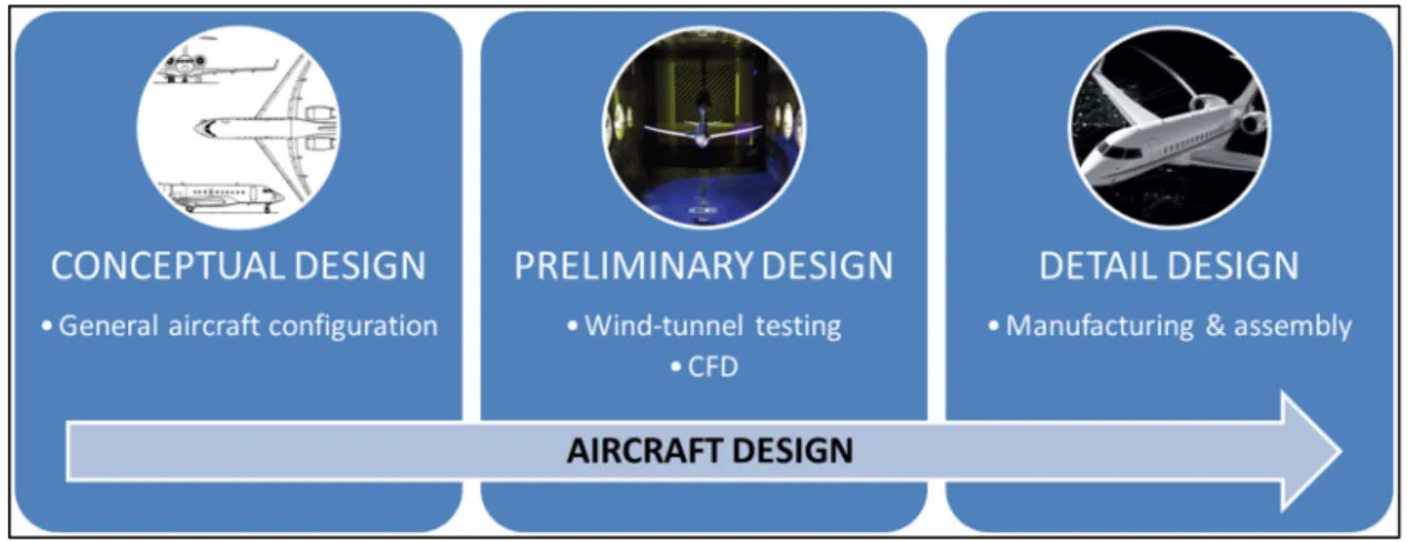
Aircraft design is the engineering process of creating a flying vehicle that meets a series of specifications and requirements, generally established by an aircraft manufacturer. Occasionally, these aircraft designs may be part of scientific investigations to explore innovative technologies. Conceptual design, preliminary design and detail design are the three subsequent phases of this engineering process (Anderson, 1999). A general aircraft configuration layout should be the result from the conceptual design phase. This configuration is then subject to minor changes during the preliminary design phase. At this point, substantial wind-tunnel testing will be carried out in combination with the application of computational fluid dynamics (CFD) simulations to verify design requirements and unveil any potential design flaws that may drive configuration changes, as part of experimental test cycles much like those presented by Blackwell (1982). At the end of this preliminary design phase, the aircraft configuration should be precisely defined before committing to the endeavor of manufacturing a full-scale aircraft. The detail design phase consists of defining the necessary elements that will concern the manufacturing and technical assembly of the aircraft, literally this would be the “nuts and bolts” phase of the design. This concludes the design process, which is followed by prototype manufacturing, flight test, certification and production.
This research project has a particular interest in the preliminary design phase of contemporary transport aircrafts, specifically in one of the main tools employed at this stage, wind-tunnel testing. It will also explore its relationship with CFD. Over the last 40 years, the development of CFD has been partially responsible for the reduction in the use of wind-tunnel tests. As a result, a number of wind tunnels have been decommissioned. Nevertheless, wind-tunnel testing continues to be paramount to the aircraft design process to test flight configurations at subsonic speed and high angle-of-attack, characteristic of take-off or landing. A good example would be the determination of the maximum lift coefficient 𝐶 . For an aircraft at a given speed, lift increases almost linearly until its maximum at a critical value of the angle of attack, the stall point, before dropping as a consequence of flow separation at high incidence. Understanding aerodynamic behavior during stall is a very important phase of the design of any aircraft. However, the flow complexity when separation begins to develop close to the stall point makes predicting 𝐶 mathematically very complicated (Tinoco et al., 2005). Therefore, CFD cannot be used autonomously to develop high-lift system details if the adequate prediction of maximum lift cannot be made. Under these circumstances, common CFD simulations would fall short and the use of wind-tunnel testing would be required. Aircraft manufacturers know the importance of such an essential tool and very rarely would they fly a vehicle that has not been previously tested in a wind-tunnel.
As wind-tunnel testing continues to have a powerful impact on the aircraft design process, there is interest in how to improve the accuracy of tunnel tests results. The National Research Council of Canada (NRC) Trisonic Wind Tunnel (TWT) is a perfect example of a facility with outstanding capabilities that, after over fifty years of operation, still continues to invest in its own development and improvement. Even though the notable performance of this facility is undeniable, the fidelity of its test results can further be refined within specific test conditions. Take, for instance, low-speed tests investigating the behavior of an aircraft model at high angle-of-attack, where the complexity of the flow around the test article challenges the ability to obtain high definition results in such an important section of the aircraft performance envelope. In this context, it is worth the effort to explore how to enhance the current capabilities of the TWT to refine test results. The research project described by this
dissertation focuses on the improvement of wind-tunnel wall corrections at the NRC TWT, particularly when testing semispan models at low-speed.
0.1 History and background
The history of the wind tunnel goes back to the numerous experiments carried out towards the end of the nineteenth century to try and understand aerodynamics. Before that, most of these experiments employed whirling arms, first used by Benjamin Robins to study basic geometries (Baals, 1981). A typical whirling arm would mount any given test geometry to its end, and when moved through still air in a centrifuge motion, one could study its aerodynamic behavior. Later on, Sir George Cayley also used a whirling arm to obtain the necessary test data to build a small glider, believed to be the first heavier-than-air vehicle to successfully fly.
It was not until the early 1900’s when the first wind tunnels started to be commonly used by aeronauts. Wilbur and Orville Wright, in their quest to create their renowned aircraft, were forced to reject the existing aerodynamics handbook and trust their own data. The Wright brothers built a wind tunnel in 1901 with a simple design that allowed them to measure the relative lifting forces on a test article. The results encouraged the Wrights to build a bigger and more sophisticated wind tunnel with a 16-inch square section that provided them with all the necessary data to conceive their 1903 Wright Flyer.
After the Wright brothers’ achievement in the United States, Europe closely followed by funding the construction of a series of major wind tunnels which led to a European technical leadership in aviation between 1903 and 1914. This is the reason why the two basic types of wind tunnels are named after European scientists. The open-jet version of the open-return wind tunnel also gets the name of Eiffel tunnel, after the French engineer Gustave Eiffel. The German aerodynamicist Ludwig Prandtl gave his name to the closed-return or Göttingen type tunnel.
In the following years, the construction of the US Navy wind tunnel in 1916 at the Washington Navy Yard and the tunnel built in Paris by ONERA in the early 1930’s were the
most remarkable activities in the field. During World War II, Germany made significant progress in wind-tunnel technology by building at least three different supersonic facilities, one of them able to reach Mach 4.4 air flows. At the end of WWII, in 1946, France rebuilt an Austrian dismantled wind tunnel that still is operated today by ONERA as the world largest transonic wind tunnel. The US also built eight new wind tunnels, including the National Full-Scale Aerodynamics Complex (NFAC) at NASA Ames, currently the world’s largest wind tunnel located in Mountain View, California.
The National Aeronautical Establishment (NAE), founded in 1951 and known today as the aerospace division of the National Research Council (NRC Aerospace), coupled with the construction of several wind tunnels, promoted Canada as a world-class aerospace nation. Motivated to develop high-speed aircraft like the Arrow program, the Canadian government built one of its most relevant testing facilities, the 5ft Trisonic Blowdown Wind Tunnel in Ottawa (Nelson et al., 2004). Since becoming fully operational in 1963 (Ohman, 2001), this facility has hosted projects for clients such as Bombardier, the Department of National Defense (DND), NASA and other major airframers and research entities.
Since the emergence of computational fluid dynamics (CFD) at the end of the 1960s, the increasing role of numerical simulations has influenced the way wind tunnels are used in the aerospace design process. The advances in computational capabilities, development of new algorithms, and cost disparity between numerical and experimental techniques have favored an aggressive use of CFD, resulting in the reduction in wind-tunnel time for aircraft development programs (Chapman, 1979). Sources like the RAND report (Anton et al., 2014) recognize CFD as a contributor to a reduction of about 50 percent of required wind-tunnel testing hours for applications such as transport aircraft tests at cruise conditions. Since 1980, NASA alone has closed over 20 wind-tunnel facilities (Malik and Bushnell, 2012). However, while reliable in typical cruise flow conditions, computational fluid dynamics (CFD) struggles to accurately predict separated flow regions for aircraft applications. For this and other complex flow applications, wind-tunnel testing continues to be the backbone of the aeronautical development process (Kraft, 2001). Today, the discussion needs to focus on how CFD and wind-tunnel testing can be integrated to increase productivity in aerospace design.
Although CFD is a useful tool for identifying options in the preliminary design of an aircraft, authors like Goldstein (2010) describe how wind tunnels are still needed to gather the data in situations where significant turbulent flow develops around complex geometries. A typical example of this synergy is the use of CFD in pre-test planning to optimize the use of the wind-tunnel facility. Additionally, computational methods can be used in parallel with experimental testing to assess and study wind-tunnel effects such as wall interference.
0.2 Scope and approach
This section intends to serve as a guide to the contents presented in this dissertation. As briefly introduced before, this work studies how wind-tunnel wall corrections at the NRC TWT may be improved, particularly when testing semispan models at low-speed, and how experimental and numerical data can be used in combination to achieve this goal.
The first chapter will provide an overall perspective of important concepts to wind-tunnel testing like scale effects, flow similarity and wall interference. It will introduce the main factors that determine the relevance of wall interference, such as flow velocity or type test article, using them as a frame of reference to the considered research project. Then, the tools employed to rectify such interference will be described. In particular, the concept of wall corrections, their classification, computation techniques and specific wall-correction methods applied at relevant facilities will be reviewed. Special attention will be given to the one-variable method, the wall-correction method applied at the NRC TWT. At the end of this chapter, the problem statement addressed in this dissertation will be presented following a preliminary analysis of the one-variable method based on some available experimental data from the Bombardier Global 6000.
The primary goal of this research project is the update of the one-variable method, as it will be presented in the second chapter, together with the complementary secondary objectives that will be sought to contribute to that main goal. The methodology to achieve the desired results will be detailed in the third chapter. Details about the development of an offline test bench that was used throughout the entire research project will be also provided in this chapter. This offline tool efficiently computes wall corrections using the one-variable method
without the need to access and re-process wind-tunnel raw data. The three different model geometries employed during this research are the Bombardier Global 6000, the NRC NACA0012 Symmetrical Calibration Wing and the NASA Common Research Model (CRM); all of them in a half-model configuration. These models will be presented together with the particular applications given to the experimental data obtained using each of them as a test article. Special attention is given to the NASA CRM, for which both experimental tests and numerical simulations were performed. The methodology section will conclude by explaining how CFD results will be used to achieve the project goals and establishing the criteria to determine the validity of all the updates applied to the one-variable method.
The fourth chapter will present the results generated during the process of updating the wall-correction methodology. It will begin by studying the influence of several test parameters over an offset issue described as part of the problem statement. Then a CFD-based validation of the current wall-correction methodology as a whole, in the context of the criteria defined in the methodology chapter, will be presented. The results chapter will then propose an update to the potential theory representation of a semispan tunnel model’s fuselage and wing, which will be validated using free-air CFD results for the particular case of the CRM at the NRC TWT. The advantages of using these updates will be gauged in terms of the overall improvement to the wall corrections. The fourth chapter will continue presenting wall corrections from an experimental data set using the CRM at the NRC TWT with a solid-wall test boundary that was corrected using free-air simulations of the same model in the same conditions. The end of the results chapter presents an application of the techniques applied in this project for tests performed in transonic flow conditions. Finally, the last chapter will review the work completed to validate and update the one-variable method and suggest some further advances that can be performed, particularly improvements to the methodology in transonic flow conditions at the NRC TWT.
CHAPTER 1
LITERATURE REVIEW AND STATE OF THE ART
The ultimate goal of testing a new aircraft at the preliminary design stage is to determine its operational limits and verify whether its original design specifications and requirements will be met at the production phase. At that final stage, the product will be a full-scale aircraft capable of flying within the desired operational envelope. In general, differences between test results obtained from a scaled aircraft model and a full-scale production aircraft ploughing through the sky can be attributed to scale effects. Rae and Pope (1984) focus on presenting scale effects as the differences that arise when the fluid dynamic dimensionless parameters are not the same in the experiments than in actual flight operation. Others like Bushnell (2006) reflect on other reasons for concern when scaling from wind-tunnel to flight, such as mounting effects, aeroelastic distortion, geometric fidelity or wind-tunnel walls, the latter being of great importance to this dissertation. In addition to presenting the scale effect problem, Blackwell (1982) introduces several ways to cope with the problem of wind-tunnel to flight Reynolds number disparity.
When it comes to the huge difference in terms of size between a scaled model and a full-scale aircraft, flow similarity plays a very important role to ensure the data obtained from the scaled test article is meaningful for the full-scale case. In general, flows around two differently sized models of the same flight vehicle are considered to be similar if Reynolds and Mach numbers can be matched (Anderson, 1984). Flow similarity is of great importance in wind-tunnel testing applications.
To ensure that the flow physics of a wind-tunnel model match those of its full-scale version, sufficiently high chord Reynolds numbers are usually required. This can be achieved in wind-tunnel testing by different strategies (Figure 1.1), such as using large scale models, pressurizing the tunnel to run tests above atmospheric pressure (higher pressure means higher fluid density according to the equation of state) or resorting to a cryogenically cooled test
medium to benefit from the advantageous properties of gases at low temperature (lower viscosity, higher density and lower speed of sound) described by authors like Kilgore et al. (1974). Another possibility to obtain higher Reynolds numbers is to play with the viscosity parameter by operating the wind-tunnel exchanging fluids between the actual and the test conditions, for instance, using nitrogen or water instead of dry air.
Figure 1.1 Different approaches to obtain high Reynolds number by adjusting
wind-tunnel testing parameters
The use of higher than full-scale test velocity is also an option to reach high Reynolds numbers. This allows using smaller scale models in wind tunnels where model size is a constraint. Of course this may affect the similarity of the flow since the Mach number is not matched anymore. However, for low Mach number applications this is less critical (Katz and Plotkin, 2001), provided assumptions like incompressible flow (discussed later in this chapter) are not violated.
In addition to considering flow similarity to deal with scale effects, a scaled model tested in a wind tunnel also experiences the influence of the test section walls. In a very simple way, wall interference may be described as the difference between the wind-tunnel flow field and its free-air counterpart (Figure 1.2). Wall interference is a test section specific bias error in wind-tunnel test data.
Figure 1.2 Wall interference described as the difference between the wind-tunnel and free-air flow fields.
This interference originates from the longitudinal static pressure gradient in the tunnel test section and along its boundaries, which produces a series of forces that need to be subtracted out. In order to rectify this phenomenon and obtain the aircraft free-air behavior, wall interference must be calculated and a series of wall corrections must be applied.
1.1 Main factors of aerodynamic interference in wind-tunnel testing
As part of the Advisory Group for Aerospace Research and Development report published in 1998 (AGARDograph 336), Krynytzky and Hackett consider that the severity of wall interference is driven by several factors including (1) flow speed, (2) type and size of the test article, (3) type of test section walls and, in general, (4) the nature of the aerodynamic forces generated by the test article. This section will discuss each of those factors.
1.1.1 Flow speed
As previously introduced, flow similarity needs to be ensured to correlate scaled model test results to full-scale. In wind-tunnel testing applications, Mach and Reynolds numbers are the most relevant correlation parameters to consider. If testing at low-speed, the Mach number dependence of the governing equations of fluid dynamics is small enough to be neglected.
Aside from high-lift (take-off/landing) configurations, this is generally considered to be the case for Mach numbers lower than 0.3, where the principles of low-speed aerodynamics are generally applicable.
Low-speed aerodynamics
At low-speed Mach, the Reynolds number becomes the main parameter of interest for similarity and the flow is considered to be incompressible. For incompressible flows, density ρ is considered to be a constant. When this constant density condition is applied to the continuity equation, the outcome is that the divergence of the flow velocity field is zero, as seen in Eq. (1.1).
+ ∇ ∙ (𝜌𝑉⃗) = ∇ ∙ 𝑉⃗ = 0 (1.1)
Additionally, if the flow viscosity µ is low enough to be considered to be zero, the Reynolds number will be infinite and the flow can be considered inviscid. In an inviscid fluid, irrotational motion is permanent (Milne-Thomson, 1966). An irrotational flow around a streamlined body has zero vorticity or, what is the same, the curl of the velocity field is zero (∇ × 𝑉⃗ = 0). From vector analysis, a vector with zero curl must be the gradient of a scalar function. In the case of the velocity field 𝑉⃗, that scalar function is called velocity potential 𝜙, where 𝑉⃗ = ∇𝜙.
Therefore, for low-speed irrotational flows, the Laplace equation, Eq. (1.2), is satisfied and may be derived as follows.
∇ ∙ 𝑉⃗ = ∇ ∙ ∇𝜙 = ∇ 𝜙 = ∆𝜙 = 0 (1.2)
In summary, for an inviscid, irrotational flow, the velocity field 𝑉⃗ is the gradient of the velocity potential 𝜙. This velocity potential is also known as potential flow. If the flow is also incompressible, the velocity potential satisfies the Laplace equation (∆𝜙 = 0) and potential theory may be applied (Rae and Pope, 1984). All these concepts will be relevant for the use of potential theory.
Potential theory
Low-speed inviscid flows around streamlined bodies, like the ones investigated in this research project, may be represented by means of singularities (fundamental solutions) of the Laplace equation. The discipline that studies how to combine those singularities into a potential flow 𝜙 model is called potential theory.
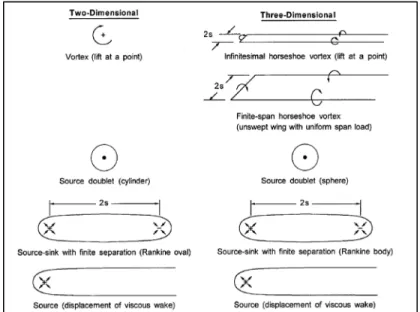
Based on their particular application, most potential flow models employ complex combinations of basic singularities such as sources, sinks and vortices (Figure 1.3) to represent the lifting and non-lifting effects of the streamlined body. The non-lifting effects, known as blockage effects, are a combination of the contribution of the body’s volume and wake. Authors such as Krynytzky and Ewald (1998) approach the use of different singularities and singularity-distributions to best represent the flow around the specific geometry studied.
Figure 1.3 Elementary singularities of the Laplace equation in potential flow models. From: Krynytzky and
As noted by Hackett et al. (1979), in general, volume effects (solid blockage, 𝜖s) can be
represented by a distribution of point doublets (source-sink pairs) and wake effects (wake blockage, 𝜖w) can be represented by sources. Additionally, lifting effects can be represented
by horseshoe vortices or semi-infinite line doublets, as presented by Ulbrich (1998).
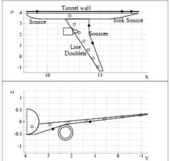
All levels of complexity may be achieved by combining different singularities into a specific potential flow model. A simple body of revolution may be modelled with just a source and a sink located at a distance from each other. Figure 1.4 shows an example of a simple array of singularities used by Iyer and Everhart (2001) to represent the flow around an aircraft wind-tunnel model tested at NASA Langley. More complex geometries may be modelled using potential theory. As Rae and Pope (1984) indicates, the use of the currently available computing technology allows models to be made up of thousands of singularities.
Figure 1.4 Example of a potential theory representation for an aircraft wind-tunnel model. From: Iyer and Everhart (2001).
Once the potential flow model 𝜙(𝑥, 𝑦, 𝑧) around a specific streamline body has been defined, the velocity components, Eq. (1.3), may be obtained by derivation.
u = ; v = ; w = (1.3)
The use of potential theory is paramount to some of the wall-correction methodologies applied at different wind tunnels, which is why it is key for this entire dissertation. When flow viscosity is not an issue or when dealing with thin boundary layer, a detailed potential flow model can provide a proper representation of the flow behavior around a flying vehicle in free-air.
Viscous effects
Unfortunately, potential theory is not applicable in all circumstances. For instance, wind-tunnel tests at low-speed Mach numbers and high incidence, typical of take-off and landing conditions, generally experience the additional challenge of the development of flow separation over the test article. These conditions result in zones experiencing significant adverse pressure gradients where complex separated flows with high viscosity and vorticity develop. The significant viscous forces and the vorticity void the inviscid and irrotational flow conditions assumed for the low-speed aerodynamic scenarios discussed so far. Consequently, when significant flow separation is present, the traditional use of potential theory as a tool to obtain solutions of the flow behavior is not valid.
The effects of flow separation over streamlined bodies include increased drag as well as a reduction of the pressure differential, resulting in reduced lift. Hoerner (1975) highlights the importance of investigating the stall properties of an aircraft and its relationship to relevant design variables such as aspect ratio, sweep angle, load distribution or planform. The ability to provide accurate results in stall conditions, where flow separation is significant, is paramount in the preliminary design phase of any aircraft.
1.1.2 Wind-tunnel models
At the beginning of this chapter, the necessity to obtain high enough Reynolds numbers to guarantee flow similarity when testing scaled models at low-speed was introduced. The use of larger scale models has been presented as a solution to this problem. A complementary technique for reaching higher chord Reynolds numbers at a given test facility is the use of semispan or half-models mounted on a solid plate over one of the tunnel walls, instead of full-span models mounted to a strut. Franz (1982) discusses in detail the application of half-models in wind-tunnel testing, as well as its benefits and drawbacks. Although semispan wind-tunnel models allow reaching the desired high Reynolds numbers, their larger size with respect to the tunnel cross section and proximity to the tunnel boundary accentuates the wall-interference effects.
Semispan models
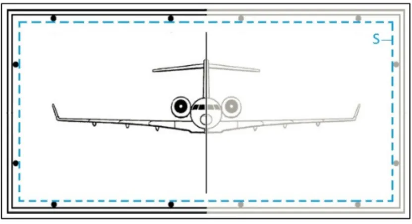
Using the semispan or half-model approach allows for the building of larger scale models (Figure 1.5), which can easily fit the measuring instrumentation needed in the model for wind-tunnel testing such as pressure taps or balances. Additional advantages when using half-models include lower construction cost, compared to full-span models, and higher model geometric fidelity.
Figure 1.5 Sketch of a full-span model (left) and a semispan model (right) of an aircraft in the same test section. Notice the higher model span-to-tunnel width
Unfortunately, their main disadvantages are a large wall-interference effect compared to full-span testing and the effects of the side-wall boundary layer over the attached half-fuselage, which can be minimized by using splitter plates or standoffs, as pointed out by authors like Blackwell (1982) or Gatlin et al. (1997), to relocate the model at a distance where better flow quality can be provided. The severity of wall-interference effects experienced in half-model tests is related to the larger model size to test section size ratio (larger models are unavoidably closer to the tunnel walls) and must be rectified by applying wall-interference corrections.
Ultimately, wind-tunnel results using both full-span and semispan models should correlate when the data are adequately corrected for interference, as proved by authors like Gross and Quest (2004).
1.1.3 Wind-tunnel design
Every wind tunnel has some distinctive and unique features that make it capable of attaining the specific flow conditions required for the testing it is designed to host. In general, all of them may be classified in terms of tunnel and test section types. There are two basic types of wind tunnels, open circuit and closed circuit (Rae and Pope, 1984). For each of them, their test section may be open, partially open (perforated or slotted-wall) or closed.
Aside from that general classification, special consideration must be given to minimizing problems derived from wall interference when selecting a particular wind tunnel for an experiment, as presented by Blackwell (1982). Some wind-tunnel test sections may be designed to minimize the wall-interference effect. That is the case of test sections with adaptive walls or boundary layer suppression/ingestion technology. Other facilities may also rely on post-processing their data by using some kind of wall-interference correction method, like the ones that will be introduced later in this chapter. For a specific wind tunnel, all of
these features make the test article more or less sensitive to wall interference. The National Research Council 5ft Trisonic Wind Tunnel, where wall interference is minimized by both the design features of its test section and by data correction, is the tunnel considered in this dissertation.
The National Research Council 5ft Trisonic Wind Tunnel
Located at the Uplands Road facilities in Ottawa, the NRC 5ft tunnel (Figure 1.6) is an open-return tunnel of the blow-down type. Unlike regular open-return wind tunnels, where air is drawn through the tunnel by suction, blow-down wind tunnels are a special kind of open return tunnels that operate by blowing air downstream for short periods of time. The Mach number range in this tunnel goes from low subsonic at 0.1 to a maximum of 4.25 (Ohman, 2001).
Figure 1.6 Overview of the NRC 5ft Trisonic Wind Tunnel.
The tunnel 8.4 MW (11,250 hp) compressor plant is used to charge the storage tanks with 40 tons of dry air at 21 atm and 21°C. When initiating a run, the control valve opens and the air flows through the settling chamber where a series of flow stabilizing devices, noise
attenuating devices and turbulence damping screens ensure quality air flow before it goes through a flexible nozzle that supplies air up to 17 atm to the closed 5ft by 5ft square test section, surrounded by an enclosed plenum. Finally, the air flow goes through a diffuser, a silencer and an exhaust where it is extracted at atmospheric pressure. Although run times are dependent on test conditions, a typical run can last about 20 seconds then taking around 20 minutes to recharge the air tanks. As described in Elfstrom et al. (2001), this facility has the capability of operating using the abovementioned 5ft by 5ft test section for 3D testing or a 1.25ft by 5ft test section for 2D testing, easily interchangeable thanks to its “roll-in roll-out test section system”. Only operation in the 3D test section will be considered for the remainder of this dissertation.
In order to perform tests with a partially-open boundary, the 3D test section walls are perforated by 0.5 inch diameter holes inclined 60° toward the oncoming flow (Figure 1.7) and equipped with splitter plates for edge tone suppression (Dougherty et al., 1976). During ventilated-wall tests, the porosity in the walls can be adjusted from 0.5% to 6% by an external throttle plate. Porosity (or other forms of partially open boundary) is a necessity for transonic testing (Rae and Pope, 1984); it prevents choking at the near-sonic Mach numbers and prevents shock and expansion wave reflections at the low supersonic Mach numbers. At this facility, low-speed testing is also performed with the perforated boundary. A 1.5% porosity configuration is typically selected to (passively) reduce the wall interference. The use of the perforated test section with its complicated cross flow characteristics rules out the use of the standard textbook correction techniques. Solid-wall tests can also be performed in the test section on an ad hoc basis by appropriately taping the test section wall perforations, as first tested by Broughton (2013). Within this project, both solid-wall and ventilated-wall tests will be considered in subsonic flow conditions.
Figure 1.7 Detail view of the wall perforations in the NRC 5ft wind-tunnel test section.
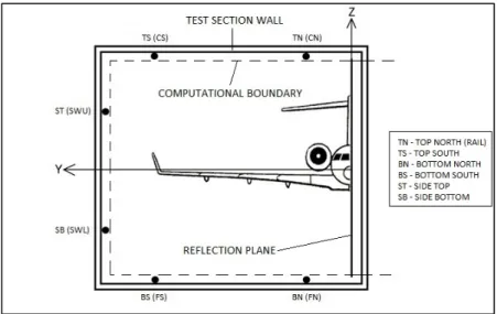
This research will study the wall interference on half-model tests at subsonic flow. For half-model tests, the model is mounted on a solid plate (reflection plate) covering one of the side walls, hereafter the “north” wall, with a splitter plate on its upstream edge. The interaction of the reflection plate boundary layer with the flow over the fuselage is minimized by the use of a filler plate that creates an appropriate stand-off distance from the reflection plate. Unlike other facilities like the NASA Ames 11ft Transonic Wind Tunnel (TWT), where pressure orifices are directly drilled at the test section boundary (Boone and Ulbrich, 2002), NRC 5ft TWT uses six pressure rails located along the test section on the ceiling, floor and south walls to measure the static pressure. These measurements are needed to determine the wall interference (Mokry, 2006). The layout of the six pressure rails can be observed on Figure 1.8.
Figure 1.8 Layout of the reflection-plate and pressure rails in the NRC 5ft wind-tunnel test section.
A six-component sidewall balance is used to measure overall forces and moments relative to the model axis. The balance is installed on the north side of the wind tunnel, supported between bearings in the test section wall and the plenum shell. The balance incidence drive motor and gearbox assembly are mounted outside the plenum. Balance excitation and sampling frequency is typically set to 10 volts and 100 Hz, respectively.
1.1.4 Nature of the wind-tunnel test
Consider a given flow speed, test section design and test article. Even in these somewhat fixed conditions, not all wind-tunnel tests are equally sensitive to wall interference. For instance, wind-tunnel tests simulating low-speed take-off, approach and landing conditions experience more complex flows that require accurate wall corrections.
To allow this section to serve as a recapitulation, this project will involve low-speed wind-tunnel tests using the semispan model of a transport aircraft mounted in the NRC 5ft
TWT with a solid-wall test section boundary. Even with all these parameters defined; the effect of wall interference will still depend on other test variables such as the model incidence.
These factors indicate that considerable wall interference will be experienced. This interference needs to be rectified through the use of wall corrections.
1.2 Wind-tunnel wall-interference correction
In a wind tunnel, the distance of the test section boundaries relative to the test article may cause an effect over the flow properties, such as flow speed or angularity (Rae and Pope, 1984). To ensure an accurate description of wind-tunnel data, the interference generated as a consequence of the presence of the tunnel walls must be understood and rectified using wall corrections. Properly corrected data can then be compared to data from different tunnels or to a free-air situation.
Publications like AGARDograph 109 (1966) and ESDU 95014 (1995), which have their foundations in the work of Glauert (1933) and other aerodynamicists that investigated boundary interference in the 1920s and 1930s, may serve much like a handbook to determine wall corrections even before the wind-tunnel test is executed. These corrections will often be referred to as “textbook”, “handbook” or “theoretical” corrections in this dissertation. These textbook corrections rely on assumptions like idealized boundary conditions and apply traditional techniques like the method of images; requiring model and tunnel geometry, measured lift and drag values (or estimated values).
When the test section boundaries have properties that cannot be modeled simply (e.g. porosity) or flow complexity is significant, textbook corrections are typically replaced with methods that include additional experimental flow measurements at the boundary, like those developed by Ashill (1993), Ulbrich (1998) or Mokry (1987); introduced later in this chapter. These methods are not limited to any particular wall boundary condition, so they can also be used with solid-wall boundaries.
The different types of wall corrections, as well as the available tools to help calculate them will be introduced in this section.
1.2.1 Classification of wall corrections
Wall corrections are categorized (Table 1.1) as presented by Garner in AGARDograph 109 (1966). First order corrections consider the most important wall-interference effects that can be addressed by blockage and incidence corrections. These corrections are given as a mean adjustment to Mach number and the angle of attack at a specific reference point, required for the model aerodynamics measured in the test section to be transferable to a “free-air” situation. Higher-order methods may be calculated to provide the gradients of the corrections over the entire test article, as described by Taylor and Ashill in AGARDograph 336 (1998).
A. First-order corrections – Blockage and incidence corrections
Blockage corrections try to compensate the volume (solid blockage) and wake (wake blockage) effects of the test article confined in the wind-tunnel test section. Solid blockage is the result of the interaction between the test section boundaries and the physical volume of the test article. In other words, it is the effect of the test section boundaries altering the distance between the streamlines in the vicinity of the test article compared to a free-air situation. In closed-jet wind-tunnels, this forces the air to flow through a smaller area as compared to a free-air scenario, which increases the air velocity around the model (Maskell, 1963). Wake blockage is caused by the wake generated by the test article, where the mean velocity is much lower than the free stream. In a closed tunnel, this results is an altered flow velocity and pressure around the model, which needs to be rectified.
Blockage corrections are represented by the blockage factor ϵ, Eq. (1.4), which is the ratio between the axial velocity increment due to the tunnel walls ΔU (or interference axial
velocity u ) and the flow reference velocity U (Rae and Pope, 1984). Corrections for dynamic pressure Δq and Mach number ΔM can be obtained from the blockage factor, as seen in Eqs. (1.5) and (1.6). The magnitude of blockage corrections can be related to the type of wind-tunnel test section boundary considered. In solid-wall tests, blockage corrections generally have greater values than in ventilated-wall tests. In addition, the sign of blockage corrections is positive in solid-wall tests and typically negative in ventilated-wall tests.
ϵ =u
U (1.4)
∆q = q(1 + ϵ) (1.5)
∆M = 1 +κ − 1
2 M ϵ M (1.6)
The flow angle on the model is also influenced by the presence of the tunnel walls; therefore the angle of attack needs to be corrected using incidence corrections. Different formulae to calculate the incidence correction may be derived for specific test section geometry, as explained by Garner (1966). In general, the angle of attack correction ∆∝ is obtained as a function of the interference upwash velocity Δw (or w ) and the tunnel reference velocity U at a given reference point in the test article (Krynytzky and Ewald, 1998), as seen in Eq. (1.7). For positive lift, the angle of attack correction is positive in solid-wall tests and usually negative for ventilated test sections.
∆∝=w
U (1.7)
B. Higher-order corrections
Depending on the client’s test goals, higher-order corrections may be applied to wind-tunnel test data as a function of the first-order corrections. Higher order corrections, such as pitching moment corrections ∆C or buoyancy drag corrections ∆C , take into account the fact that first-order corrections are not constant at different points on the model. Pitching moment corrections for a wing may be calculated as a function of the spanwise or chordwise variation
of the angle of attack. Buoyancy drag corrections can be computed as a variation of the blockage factor along the fuselage (Taylor and Ashill, as part of AGARDograph 336, 1998).
Table 1.1 Classification of wall corrections.
FIRST-ORDER CORRECTIONS
• Rectify most important effects of wall interference. • Calculated at selected reference point.
• Blockage (Δq and ΔM) / Incidence (∆∝) HIGHER-ORDER
CORRECTIONS
• Rectify first order variation effects throughout the model. • ∆C or ∆C are common examples
As a visual example, let’s consider the illustration in Figure 1.9, where the angle of attack correction for a certain aircraft model in a wind tunnel is plotted on a XY plane. Typically, the wind-tunnel client would receive first order corrections, i.e., blockage and incidence corrections, at a specified reference point. Additionally, the client could request higher-order corrections such as pitching moment correction ∆C based on the variation of ∆∝.
Figure 1.9 Contour plot showing the variation of the angle-of-attack over a tunnel model to illustrate the concept of first and higher order corrections.
1.2.2 Wall-correction calculation techniques
The effect of wall interference on a model tested in a wind tunnel may be calculated using three different approaches for wall-correction computation techniques. All of them require the exact location of the model in the test section as well as information about the test section boundary conditions.
A. Analytical techniques
Analytical techniques apply potential theory to compute wall interference. They are based on solutions of the linearized potential equation of the wall-interference flow field (Milne-Thomson, 1966), Eq. (1.8), where 𝜙 is the interference velocity potential near the walls.
(1 − M) ∂ 𝜙 ∂x + ∂ 𝜙 ∂y + ∂ 𝜙 ∂z = 0 (1.8)
By introducing the compressibility factor β of Eq. (1.9) and applying the Prandtl-Glauert transformation, Eq. (1.8) becomes the Laplace equation and potential theory may be applied. At low-speed tests, β is expected to be close to one.
β = 1 − M (1.9)
Given that the wall interference is a “far-field” effect (Mokry, 2006), a priori it is not necessary to represent in detail the test article geometry and singularities of the Laplace equation such as sources, sinks or doublets can be used to represent the model. Analytical techniques include the method of images, which can be applied to wind tunnels with rectangular solid-wall test sections.
Method of images
Previously in this chapter, the use of potential theory to represent the unbounded flow around a streamlined body was introduced. However, there are times when the flow around that body is disturbed by a nearby boundary.
Assuming a wind tunnel has a constant rectangular cross section extending far enough both upstream and downstream from the model and provided that the nearby boundary satisfies the no-flow-through condition, like in the case of a model tested in a wind tunnel with a solid-wall test section, it is appropriate to apply analytic techniques such as the method of images as described by Krynytzky and Ewald in AGARDograph 336 (1998). In wind tunnels where the model is located on the centerline of the test section, symmetry conditions can help simplify the analysis and determine the interference velocity and, by extension, wall-interference corrections.
Historically, wind-tunnel wall interference is taken into account by using potential theory method of images suitably arranged for the test section geometry and boundary conditions. By applying this method, the flow field created by certain singularities in the vicinity of a solid boundary can be simulated by superimposing mirror image singularities; this guarantees that there is no flow in the symmetry plane at the actual boundary location (Kuethe and Chow, 1986).
Figure 1.10 Vortex near a solid boundary and image vortex placed
to guarantee the no flow through condition. From: Kuethe and
For example, consider a vortex of strength Γ at distance a from a solid boundary like the one represented in Figure 1.10, located at (0, a). By placing another vortex of opposite strength −Γ at a symmetrical location with respect to the boundary, i.e., (0, -a); the normal component of the velocity would be cancelled at the wall.
As explained by Krynytzky and Ewald, the method of images may be applied to wall-interference calculations by developing a set of image singularities required to represent all the wall surfaces of a given test section and adding their effect to determine the interference on the model. As depicted by Figure 1.11, for 3D model (or half-model) testing in rectangular test sections, the image system is doubly infinite because of mutual interference of vertical and horizontal walls, which require images along the diagonals (Rae and Pope,1984).
Figure 1.11 Illustration of the method of images: Image system for a wing in a closed rectangular tunnel. From: Rae and Pope (1984).
B. Numerical techniques
Numerical techniques allow representing more complex model and test section geometries. These techniques use tools like panel codes to obtain the wall-interference flow. The wall-interference flow field is calculated by taking away the free-air flow field of the test article from the computed solution obtained in the wind tunnel.