Higher-Level Consistencies : When, Where, and How Much

(1)

HAL Id: tel-02295985

https://tel.archives-ouvertes.fr/tel-02295985

Submitted on 24 Sep 2019

HAL is a multi-disciplinary open access archive for the deposit and dissemination of sci-entific research documents, whether they are pub-lished or not. The documents may come from teaching and research institutions in France or abroad, or from public or private research centers.

L’archive ouverte pluridisciplinaire HAL, est destinée au dépôt et à la diffusion de documents scientifiques de niveau recherche, publiés ou non, émanant des établissements d’enseignement et de recherche français ou étrangers, des laboratoires publics ou privés.

Much

Robert J. Woodward

To cite this version:

Robert J. Woodward. Higher-Level Consistencies : When, Where, and How Much. Data Structures and Algorithms [cs.DS]. Université Montpellier; University of Nebraska-Lincoln, 2018. English. �NNT : 2018MONTS145�. �tel-02295985�

(2)

by

Robert J. Woodward

A DISSERTATION

Presented to the Faculty of

The Graduate College at the University of Nebraska In Partial Fulfilment of Requirements

For the Degree of Doctor of Philosophy

Major: Computer Science

Under the Supervision of Professor Berthe Y. Choueiry and Dr. Christian Bessiere

Lincoln, Nebraska September, 2018

(3)

RAPPORT DE GESTION

2015

THÈSE POUR OBTENIR LE GRADE DE DOCTEUR

DE L’UNIVERSITÉ DE MONTPELLIER

En informatique

École doctorale Information, Structures, Systèmes Unité de recherche Laboratoire d'Informatique,

de Robotique et de Micro-électronique de Montpellier (LIRMM) En partenariat international avec Université du Nebraska--Lincoln, États Unis

Présentée par Robert J. WOODWARD

Le 20 septembre 2018

Sous la direction de Christian BESSIERE

et Berthe Y. CHOUEIRY

Devant le jury composé de

Sébastian ELBAUM, Professeur, Université de Virginie

Stephen D. SCOTT, Professeur Associé, Université du Nebraska—Lincoln Souhila KACI, Professeur, LIRMM

Jamie RADCLIFFE, Professeur, Université du Nebraska—Lincoln Christian BESSIERE, directeur de recherche CNRS, LIRMM

Berthe Y. CHOUEIRY, Professeur Associé, Université du Nebraska—Lincoln rapporteur rapporteur examinatrice examinateur co-directeur co-directrice

Les Cohérences Fortes : Où, Quand, et Combien

(4)

Robert J. Woodward, Ph. D. University of Nebraska, 2018

Adviser: B.Y. Choueiry and C. Bessiere

Determining whether or not a Constraint Satisfaction Problem (CSP) has a so-lution is N P-complete. CSPs are solved by inference (i.e., enforcing consistency), conditioning (i.e., doing search), or, more commonly, by interleaving the two mecha-nisms. The most common consistency property enforced during search is Generalized Arc Consistency (GAC). In recent years, new algorithms that enforce consistency properties stronger than GAC have been proposed and shown to be necessary to solve difficult problem instances.

We frame the question of balancing the cost and the pruning effectiveness of con-sistency algorithms as the question of determining where, when, and how much of a higher-level consistency to enforce during search. To answer the ‘where’ question, we exploit the topological structure of a problem instance and target high-level consis-tency where cycle structures appear. To answer the ‘when’ question, we propose a simple, reactive, and effective strategy that monitors the performance of backtrack search and triggers a higher-level consistency as search thrashes. Lastly, for the ques-tion of ‘how much,’ we monitor the amount of updates caused by propagaques-tion and interrupt the process before it reaches a fixpoint. Empirical evaluations on benchmark problems demonstrate the effectiveness of our strategies.

(5)

DEDICATION

(6)

ACKNOWLEDGMENTS

I would like to thank Dr. Berthe Y. Choueiry and Dr. Christian Bessiere for their continued support and encouragement and for allowing me to be a part of both of research groups, namely, the Constraint Systems Laboratory (ConSystLab) at the University of Nebraska-Lincoln and the Coconut team at LIRMM and the Université de Montpellier. I treasure the friendships, conversations, and interactions with all of the people in both labs and feel honored that I could belong to both groups.

I would like to acknowledge research collaborations and the scientific input of the following individuals: Mr. Anthony Schneider for collaboration on Stampede, the ConSystLab solver, without which my research would have not been able to advance so far; Mr. Denis Komissarov laid important foundation for me being able to implement visualizations in Stampede; Mr. Ian Howell extended much of my initial visualization work (Chapter 3) into Wormhole far faster and better looking than I ever could; Mr. Nathan Stender with whom I developed the framework for enforcing multiple consistencies (Section 3.4.2), which was made more efficient in collaboration with Mr. Schneider; Mr. Christopher Reeson created the original 4PPC algorithm that I extended (Chapter 6); Mr. Daniel Geschwender was always available for help with experimental design. I am grateful to the Holland Computing Center team for their support in running all of the experiments, especially to Dr. David Swanson and Dr. Derek Weitzel.

Finally, I am grateful to my loving family, who always encouraged me to pursue my passion of Computer Science. I am especially grateful to my wife, Allison, who lovingly and patiently put up with all the late nights spent on research.

(7)

GRANT INFORMATION

This research was supported by:

• National Science Foundation (NSF) Grants No. RI-111795 and RI-1619344, • An NSF Graduate Research Fellowship Grant No. 1041000,

• An NSF Graduate Research Opportunities Worldwide grant,

• A Chateaubriand Fellowship of the Office for Science and Technology, Embassy of France in the USA, and

• The Dean’s Fellowship, Office of Graduate Studies, University of Nebraska-Lincoln.

This work was completed utilizing the Holland Computing Center of the University of Nebraska, which receives support from the Nebraska Research Initiative.

(8)

List of Figures

1.1 The stronger the consistency, the more the pruning . . . 3

1.2 Balancing the cost of search and that of consistency . . . 3

1.3 Dimensions of enforcing consistency . . . 3

1.4 The dimensions of enforcing consistency investigated in this dissertation . . . 5

1.5 Number of backtracks per depth (BpD) using APOAC as an HLC for solving problem instance pseudo-aim-200-1-6-4 . . . 7

1.6 Superimposing the number of backtracks per depth (BpD) and the three types of number of calls per depth (CpD) to APOAC as an HLC for problem instance pseudo-aim-200-1-6-4 . . . 8

1.7 A constraint graph with two cyclic biconnected components . . . 11

2.1 A hypergraph . . . 20

2.2 The primal graph . . . 20

2.3 A dual graph . . . 21

2.4 A minimal dual graph . . . 21

2.5 A incidence graph . . . 22

2.6 Triangulated primal graph and its maximal cliques . . . 24

2.7 A tree decomposition of the CSP in Figure 2.1 . . . 24

(16)

2.9 Dimensions of enforcing consistency . . . 36

3.1 The tree view [Simonis and Aggoun, 2000] _{. . . .} ₄₁

3.2 The phase-line display [Simonis and Aggoun, 2000] . . . 41

3.3 The number of each constraint check at every depth [Epstein et al., 2005]. . . 43

3.4 The result of a node visit at every depth [Simonis et al., 2010] . . . 43

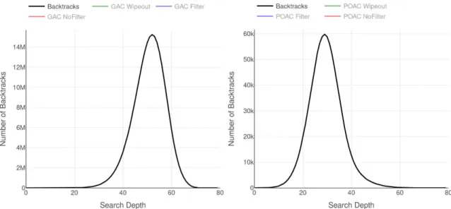
3.5 BpD for GAC (left) and POAC (right) on instance 4-insertions-3-3. . . 45

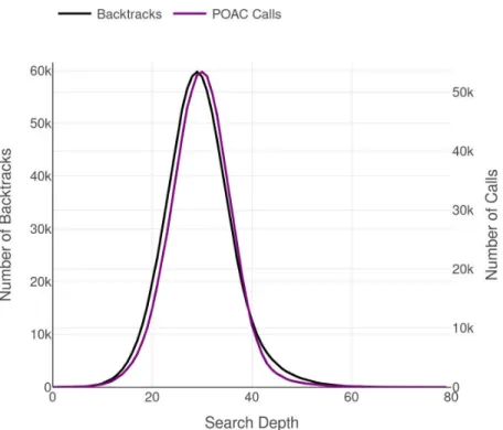
3.6 Superimposing CpD and BpD for POAC on 4-insertions-3-3 . . . 46

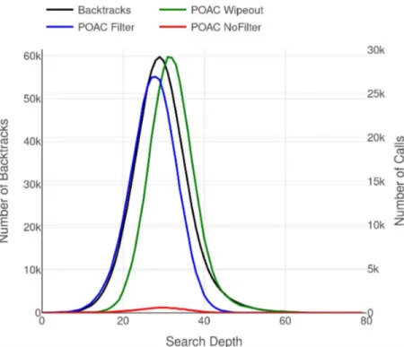
3.7 Superimposing BpD and detailed CpD (wipeout in green, filtering in blue, no-filtering in red) for POAC on 4-insertions-3-3 . . . 47

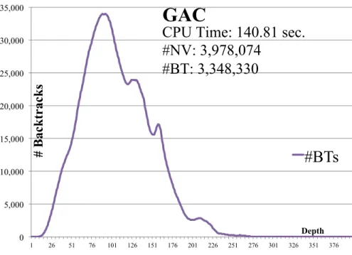
3.8 _{BpD and CpD of GAC on pseudo-aim-200-1-6-4 . . . .} 48

3.9 _{BpD (purple) and CpD’s (colored) of APOAC on pseudo-aim-200-1-6-4} 49 3.10 BpD (purple) and CpD’s (colored) of PrePeak+ _on pseudo-aim-200-1-6-4 . . . 50

4.1 Cumulative instances completed by CPU time on dom/deg . . . 72

4.2 Cumulative instances completed by CPU time on dom/wdeg . . . 73

4.3 Search progress on pseudo-aim-200-1-6-4 using dom/wdeg: GAC (top), APOAC (middle), and PrePeak+ (bottom) . . . 76

5.1 A constraint graph with two cyclic biconnected components . . . 81

5.2 A constraint graph that is a tree of cyclic biconnected-components . . . 81

5.3 A constraint graph made of a cycle of cycles . . . 82

5.4 A CSP with no solution but SAC removes no values . . . 83

5.5 The constraint graph of the CSP is a cycle . . . 83

5.6 NPOAC but not NIC . . . 87

(17)

5.8 A incidence graph . . . 87

5.9 Search progression’s past, current, and future variables . . . 110

6.1 MinFill adds the edge (i, j) because of the existing edges (i, k) and (j, k) . . 120

6.2 The sequence of triangles along the PEO of a triangulated graph . . . 120

6.3 Pruning strengths of the proposed PPC-based consistencies . . . 122

6.4 The primal graph . . . 125

6.5 Triangulated primal graph and its maximal cliques . . . 125

6.6 A tree decomposition of the CSP in Figure 6.4 . . . 125

6.7 Selecting the triangles for PPC . . . 129

6.8 Cumulative instances completed by CPU time for triggering 4P3C+ . . . 138

6.9 Selecting the triangles for PH3C . . . 143

7.1 The dimensions of enforcing consistency investigated in this dissertation . . . 153

A.1 Cumulative number of instances completed by CPU time for POAC . . . 169

A.2 Cumulative number of instances completed by CPU time for RNIC . . . 171

B.1 The constraint x1 ≤ x2. hx1, 4i is not 0.25-stable for AC. . . . 177

B.2 The relation of x1 ≤ x2. hx1, 3i and hx1, 4i are not 0.25-stable for GAC. . . . 179

C.1 A hypergraph . . . 189

C.2 The primal graph . . . 189

C.3 Triangulated primal graph and its maximal cliques . . . 190

C.4 A tree decomposition of the CSP in Figure C.1 . . . 190

C.5 A constraint graph . . . 192

C.6 A pseudo-tree of the example from Figure C.5 . . . 192

C.7 An AND/OR search tree of the example from Figure C.5 . . . 192

(18)

(19)

List of Tables

3.1 Search with GAC and POAC on 4-insertions-3-3. Note that GAC timed out . 44

4.1 The overall performance of the BTWatch strategies of Section 4.3.1 . . . 68

4.2 The overall performance of the other strategies of Section 4.3.2 . . . 69

4.3 PrePeak+ versus ‘when,’ ‘how much’ . . . 70

4.4 GAC, APOAC, and PrePeak+ on dom/deg . . . 71

4.5 GAC, APOAC, and PrePeak+ on dom/wdeg . . . 71

4.6 Representative benchmarks using dom/wdeg (time in [sec]) . . . 74

5.1 Time and memory to compute a minimum cycle basis . . . 97

5.2 Comparing computing cycles using MCB and BFSC . . . 101

5.3 Comparing lookahead using A∪bfsc_cycPOAC and A∪mcb_cycPOAC . . . 103

5.4 Lookahead with adaptive POAC techniques . . . 103

5.5 APOAC techniques on select benchmarks where APOAC beats GAC . . . 104

5.6 APOAC techniques on select benchmarks where GAC beats APOAC . . . 105

5.7 PrePeak+ with POAC techniques . . . 106

5.8 Benchmarks where PrePeak+ _{with POAC performs well} _{. . . .} ₁₀₇

5.9 PrePeak+ with POAC techniques on select benchmarks good for GAC . . . 108

5.10 Changing the r reward for PrePeak+ with ∪_cycPOAC . . . 109

(20)

6.1 4PPC variants as RFL with dom/deg . . . 134

6.2 4PPC variants as RFL on dom/wdeg . . . 134

6.3 4P3_{C on subsets of triangles at pre-processing followed by GAC as RFL} _{. . .} ₁₃₅

6.4 The performance of enforcing consistency as RFL . . . 136

6.5 The good performance of 4P3_{C as RFL on select benchmarks} _{. . . .} ₁₃₇

6.6 The performance of triggering 4P3C+ . . . 138

6.7 Comparing the filtering obtained from PPC and PH3C . . . 147

6.8 Enforcing the decision tree selections of PH3C at pre-processing followed by GAC as RFL . . . 148

6.9 4PH3C+ _{variants as pre-processing with dom/deg} _{. . . .} ₁₄₉

6.10 4PH3C+ _{variants as RFL with dom/deg} _{. . . .} ₁₄₉

6.11 _{Comparing GAC and PrePeak with 4DPH3C}+ _{. . . .} ₁₅₀

6.12 Benchmarks where PrePeak with 4DPH3C+ performs well . . . 150

A.1 Statistical analysis of weighting schemes for POAC . . . 166

A.2 Overall results of experiments for POAC. . . 167

A.3 Examples of quasi-group completion benchmark for POAC . . . 168

A.4 Examples of graph coloring, random, crossword benchmarks for POAC . . . . 168

A.5 Results of experiments for RNIC . . . 170

A.6 Examples of Dimacs benchmarks where AllC and Head perform best . . . . 171

A.7 Two graph coloring benchmarks where AllC and Head perform best . . . . 172

B.1 Number of instances completed by the tested algorithms . . . 182

B.2 Results of the experiments per benchmark, organized in four categories . . . . 183

B.3 Number of calls to STR and R(∗,2)C by benchmark . . . 184

(21)

C.2 #Instances completed fastest and average time . . . 203

C.3 Average number of goods and no-goods stored . . . 203

C.4 Average #NV . . . 204

C.5 #Instances completed fastest and average time . . . 204

C.6 Average number of goods and no-goods stored . . . 205

E.1 Primal densities for benchmark instances . . . 213

E.2 Performance of GAC2001 and STR2+ on Binary CSPs . . . 223

(22)

Chapter 1 Introduction

Constraint Processing (CP) is a flexible and effective framework for modeling and solving many decision and optimization problems in Engineering, Computer Science, and Management. In contrast to other areas that study the same problems, such as Mathematical Programming and SAT solving, the formulation of a Constraint Satisfaction Problem (CSP) allows the user to state arbitrary constraints over a set of variables in a transparent way, thus, directly reflecting the human’s understanding of the problem.

Many combinatorial problems of practical importance are commonly modeled as Constraint Satisfaction Problems (CSPs), including scheduling [Baptiste et al., 2006], resource allocation [Lim et al., 2004], and product configuration and design [Yvars, 2008]. Puzzles are whimsical and attractive tools to introduce the general public to CSPs and also to attract Computer Science students to this area of study. Examples include the Sudoku puzzle [Reeson et al., 2007; Howell et al., 2018a],1 _Minesweeper

[Bayer et al., 2006],2 _{and the Game of Set [}_{Swearingn et al., 2011}_].3

1 http://sudoku.unl.edu 2 http://minesweeper.unl.edu 3 http://gameofset.unl.edu

(23)

Research on CP dates back to the early 1960’s, and the field has matured into an independent research area in Artificial Intelligence with textbooks [Tsang, 1993;

Dechter, 2003a; Lecoutre, 2009], a handbook [Rossi et al., 2006], an association,4 _a

journal,5 _{and an annual conference.}6

To solve a CSP, CP focuses on two main directions: search and inference. In this dissertation, we use constructive backtrack search as a sound and complete algorithm for solving CSPs. Inference relies on a set of consistency properties and algorithms for enforcing them. These properties and algorithms are perhaps what best distinguishes CP from related fields that address the same combinatorial problems. They constitute the focus of this dissertation.

1.1 Motivation and Claims

Consistency algorithms operate by removing from the problem values or combination of values that cannot possibly appear in a solution to the problem. They typically operate locally on subproblems of a fixed size. As such, they typically run in polyno-mial time in the number of variables in the problem. In practice, they are interleaved with search, which runs in exponential time in the number of variables. By pruning the search tree and removing inconsistent branches and subtrees, enforcing consis-tency can significantly reduce the size of the search space. The stronger the enforced consistency, the larger the pruning (see Figure 1.1). However, the higher the consis-tency, the higher the computational cost of enforcing it. Thus, it becomes critical to decide whether it is more cost effective to spend more time exploring the search tree or pruning it (see Figure 1.2).

4_{Association for Constraint Programming (ACP),}_{http://www.a4cp.org/}_. 5_{Constraints, An International Journal published by Springer.}

6_{International Conference on Principles and Practice of Constraint Programming with}

(24)

1 n Pr un ing 1 n More pruning

Figure 1.1: The stronger the consistency, the more the pruning

Cost of Search

Cost of Consistency

Figure 1.2: Balancing the cost of search and that of consistency

In recent years, effective dynamic variable-ordering heuristics that learn during search have rendered the search cost even more sensitive to that of the algorithms for enforcing higher-level consistency (HLC), especially when these algorithms are applied systematically throughout search and uniformly over the entire network.

In this dissertation, we claim that strategies for enforcing HLCs during search can

be organized along orthogonal dimensions and we have identified three such ‘axes,’ namely, where, when, and how much of an HLC to enforce, as shown in Figure 1.3.

Where?

When?

How much?

HLC

Where?

One variable Entire CSP Always GAC Always HLC

When?

How much?

Stop early Until fixpoint

Figure 1.3: Dimensions of enforcing consistency

In summary,

• The ‘where’ axis identifies specific (or groups of) variables/constraints on which HLC is enforced

(25)

• The ‘how much’ axis indicates whether or not HLC is forced to terminated before reaching a fixpoint.

The point of origins where these three axes meet indicates the ‘strongest’ applica-tion of HLC (i.e., enforce HLC uniformly over the entire future subproblem, at each variable instantiation, and until quiescence). While such a strategy proved useful for solving difficult problem instances, the cost overhead is not always warranted. This situation yields the following question, central to this dissertation:

Where, when, and how much of a higher-level consistency should be enforced during search?

In this dissertation, we answer this critical question as follows:

High-Level consistency (HLC) properties and algorithms are instrumental for smashing the hardness of a problem instance and are cost effective:

1. When the search starts thrashing

2. Where the local structure of the constraint network has loops 3. As long as filtering and propagation are active and ‘alive’

(26)

1. Monitor the search progress to dynamically enforce higher-level consis-tency when search appears to be thrashing.

2. Identify critical cycles in the problem’s topological structure on which to restrict the application of the higher-level consistency.

3. Monitor the ‘liveliness’ of the filtering along the propagation queue and terminate propagation early and before a fixpoint is reached.

1.2 Approach

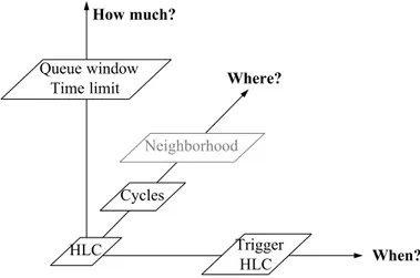
In this dissertation, we propose to combine techniques that ‘weaken’ HLC along one or more of the three axes identified above (i.e., when, where, and how much) in order to effectively prune the search space while avoiding the cost overhead and maintaining competitive performance. The main components of our techniques are as follows, see Figure 1.4: When? Where? How much? Neighborhood Cycles HLC Trigger HLC Queue window Time limit

Figure 1.4: The dimensions of enforcing consistency investigated in this dissertation

1. Monitor search to trigger HLC (see ‘Trigger HLC’ in Figure 1.4): We propose a reactive technique that monitors the amount of backtracking steps during

(27)

search as an indication of wasteful thrashing. It automatically increases the frequency of applying HLC as long it is effectively pruning the search space. Otherwise, it decreases this frequency.

2. Identify cycles to channel HLC (see ‘Cycles’ in Figure 1.4): We propose to exploit existing cycles in the constraint graph and even create new ones as structures particularly effective at localizing and channeling propagation. 3. Monitor propagation to interrupt any single execution of HLC (see ‘Queue

win-dow’ and ‘Time limit’ in Figure 1.4): We propose to monitor the effectiveness of constraint propagation by watching whether or not any filtering is obtained during a window whose width is a function of the size of the propagation queue. We also bound the maximum duration of any single call to HLC.

Below, we overview each of the proposed techniques.

1.2.1 Visualizing Search and Consistency Costs

In order to illustrate the performance of search in terms of the effort spent searching, thrashing, and enforcing consistency, we propose to visualize:

1. The number of backtracks per depth of the search tree (BpD).

2. The number of calls per depth of the search tree (CpD) to a given consistency algorithm.

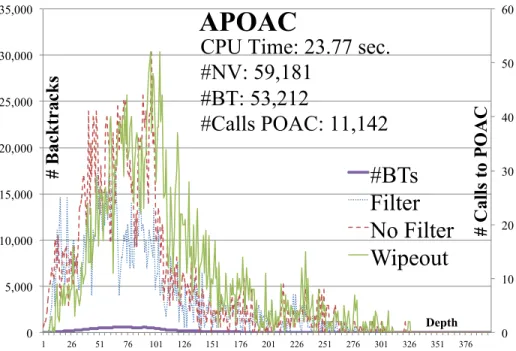
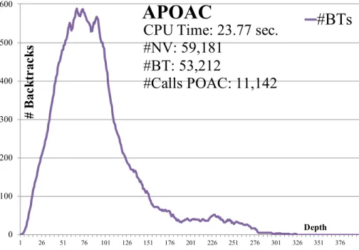
Figure 1.5 shows the BpD of a backtrack search with the consistency algorithm APOAC [Balafrej et al., 2014] for problem instance pseudo-aim-200-1-6-4 of the pseudo-aim benchmark.7

7

(28)

0 100 200 300 400 500 600 1 26 51 76 101 126 151 176 201 226 251 276 301 326 351 376 # B ac kt rac ks Depth

APOAC

_#BTs

CPU Time: 23.77 sec.

#NV: 59,181

#BT: 53,212

#Calls POAC: 11,142

Figure 1.5: Number of backtracks per depth (BpD) using APOAC as an HLC for solving problem instance pseudo-aim-200-1-6-4

Moreover, in order to illustrate the effectiveness of the consistency algorithm, we further split the CpD into three curves corresponding to:

1. Calls deemed to be extremely effective in that they prune an entire subtree and yielded backtracking

2. Calls that are not particularly effective in that they cause some pruning but do not cause a wipeout

3. Calls that are totally wasted in that they do not yield any filtering

By comparing the three CpD curves, we detect where a consistency algorithm is effective and where its efforts are wasted.

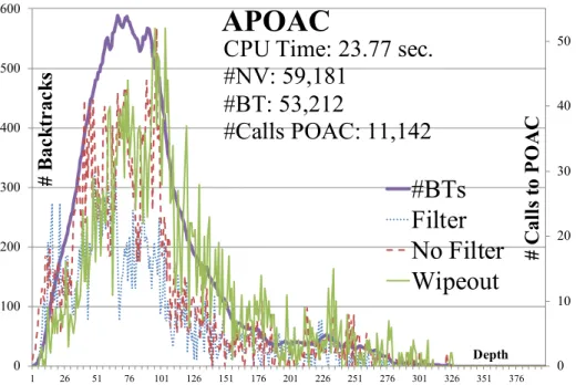
Further, the superimposition of the BpD curve and the three CpD curves provides a qualitative indication of the performance of search and of the effectiveness of a consistency algorithm. Figure 1.6 shows the superimposition of the BpD and the

(29)

three CpD curves for solving the problem instance pseudo-aim-200-1-6-4 from the pseudo-aim benchmark while enforcing APOAC. Note that:

0 10 20 30 40 50 0 100 200 300 400 500 600 1 26 51 76 101 126 151 176 201 226 251 276 301 326 351 376 # C al ls t o P O A C # B ac kt rac ks Depth

APOAC

#BTs

Filter

No Filter

Wipeout

CPU Time: 23.77 sec.

#NV: 59,181

#BT: 53,212

#Calls POAC: 11,142

Figure 1.6: Superimposing the number of backtracks per depth (BpD) and the three types of number of calls per depth (CpD) to APOAC as an HLC for problem instance pseudo-aim-200-1-6-4

• The number of backtracks is shown on the left vertical axis.

• The number of calls to HLC (i.e., POAC) is shown on the right vertical axis. • The purple line shows the number of backtracks per depth (BpD).

• The green line shows the number of HLC calls that are ‘extremely effective’ (i.e., yield wipeouts).

• The blue line shows the number of HLC calls that are ‘not particularly effective’ (i.e., filtering but no wipeouts).

• The red line shows the number of HLC calls that are ‘a total waste of effort’ (i.e., no filtering at all).

(30)

In Figure 1.6, we see that only one third of the calls to APOAC (i.e., the green curve) are really effective, which hints to the possibility of improving performance of search by ‘firing’ APOAC only when it is really effective.

We claim that this visualization is a powerful explanation tool of the performance

of search and effectiveness of an HLC and that it could even be used to allow a human user to directly intervene in the search process.

1.2.2 ‘When:’ Reactive Strategies for Enforcing HLC

In Constraint Processing, it is customary today to enforce the consistency known as Generalized Arc Consistency (GAC) at every step of the search process. As long as GAC allows search to effectively advance to deeper levels in the (tree-shaped) search space, GAC should remain the default consistency enforced. However, as thrashing occurs, we advocate to enforce stronger consistencies in order to more aggressively prune the search space and, subsequently, reduce the search effort. We propose to watch the number of backtrack steps during search as an indication of thrashing. To this end, we investigate three techniques: BTWatch, PrePeak, and PP-BTWatch:

1. BTWatch watches the number of backtrack along the search and triggers HLC whenever the counter reaches a given value, regardless of the position in the search tree.

2. PrePeak watches the number of backtracks per level of search (which is equal to the number of variables of the CSP) and enforces HLC at levels slightly shallower than the level where the peal value of the number of backtracks per level is observed.

(31)

3. PP-BTWatch is a hybrid between BTWatch and PrePeak, which watches the number of backtrack along the search and triggers HLC whenever the counter reaches a given value and the depth is before the level where a peak value of the number of backtracks per level is observed.

Further, in all three techniques, we use the same three geometric laws to update the value of the threshold for triggering HLC. The threshold value is updated in the following situations:

1. When HLC has been extremely effective (i.e., filtering yielded wipeout), we decrease the value of the threshold.

2. When HLC has not been particularly effective (i.e., some filtering but not wipe-out), we slightly increase the value of the threshold.

3. When HLC was a total waste of effort (i.e., HLC resulted in no filtering at all), we aggressively increase the value of the threshold.

Overall, all three strategies are statistically equivalent, but exploring and evaluating them improves our understanding of reactive strategies.

1.2.3 ‘How Much:’ Monitoring Constraint Propagation

We explore three directions for monitoring the effectiveness of constraint propagation. First, enforce an ordering on the elements of the propagation queue of the HLC algorithm based on the activity of a variable/constraint or a structural property (e.g., elimination ordering). Second, because an HLC call can be costly in terms of time, we interrupt the execution of an HLC and allow it to process only a fraction of its propagation queue. Finally, we impose a bound on the duration of any call to HLC.

(32)

Combining PrePeak with the above three strategies yields PrePeak+_{, which}

is the main contribution of this dissertation.

1.2.4 ‘Where:’ Channel HLC along Cycles

Figure 1.7 shows a constraint network with two cycles intersecting on exactly one variable, which is an articulation node in the graph. This network is the ‘poster

Figure 1.7: A constraint graph with two cyclic biconnected components

child’ to illustrate the importance of cycles. Indeed, instantiating the variable of the articulation node creates a chain, yielding a tractable CSP [Freuder, 1982]. More specifically, for this cycle, applying singleton arc consistency on the articulation node allows us to remove all values that do not participate in any solution (i.e., computes the minimal CSP). We theoretically characterize HLC properties that singleton-based consistencies guarantee (i.e., sufficient conditions) backtrack-free search on cactus and block graphs.

During search, we propose to exploit cycles in the constraint network of a CSP and channel constraint propagation along those cycles to improve the effectiveness of local consistency algorithms. In particular, we study two types of cycles in a constraint network, namely, a minimum cycle basis and triangles.

1.3 Contributions

In this section, we summarize our main contributions. We divide them into core contributions, which support the main claim of this dissertation, and secondary

(33)

con-tributions, which are not directly related to the main thesis but are still valuable research results. Our core contributions are the following:

1. A new visualization of the search effort [Howell et al., 2018b]. The proposed visualization tracks search progress and difficulties as well as the effort of enforc-ing consistency as a function of the depth of the search tree. This visualization has raised a sharp interest in discussions with the designers of several constraint solvers and is the topic of a new research direction in our laboratory.

2. A reactive strategy for enforcing high-level consistency [Woodward et al., 2018]. We propose trigger-based strategies for enforcing high-level consistencies only when they are needed in order to exploit their effectiveness in pruning the search space while reducing the impact of the corresponding computational overhead. Further, we provide a unifying framework based on three orthogonal dimensions of ‘when-where-how’ to characterize how approaches for enforcing high-level consistency during search operate. Finally, we validate our approach for two HLCs, namely, POAC (a variable-based consistency property) and PC (a relational consistency property).

3. New structural properties. We identify new tractability results for block and cactus shaped constraint graphs. Exploiting our results about cactus graphs, we explore the benefits of channeling constraint propagation along cycles. More specifically, we propose to restrict POAC to the cycles of a minimum cycle basis of the graph [Woodward et al., 2016a; Woodward et al., 2017] and restrict path consistency to select triangles of the triangulated constraint graph. Future work should investigate exploiting our results for block graphs.

(34)

by investigating partial path consistency [Bliek and Sam-Haroud, 1999], empir-ically evaluating it as lookahead, which has never been studied. Jégou [1993] introduces, for non-binary CSPs, a relational-consistency property, called hyper-3 consistency (Hhyper-3C), that is ‘symmetrical’ to path consistency for binary CSPs. The advantage of this property is that it allows us to operate on a special type of cycles, that is, triangles. We introduce a weakening of H3C into partial hyper-3 consistency (PH3C).8 _{We introduce the first practical algorithm for enforcing}

PH3C during search. Importantly, we show that the ‘dubois’ benchmark9 _can

be solved backtrack free using PH3C. Our secondary contributions are the following:

1. Weight-Based variable ordering in the context of a higher-level consistency [ Wood-ward and Choueiry, 2017]. Dom/wdeg is one of the most effective heuristics for dynamic variable ordering in backtrack search [Boussemart et al., 2004]. As originally defined, this heuristic increments the weight of the constraint that causes a domain wipeout (i.e., a dead-end) when enforcing arc consistency dur-ing search. We explore alternatives for the weighdur-ing scheme in the context of two consistency properties, namely, POAC and RNIC.

2. Adaptive parameterized consistency for non-binary CSPs by counting supports [Woodward et al., 2014]. Balafrej et al. [2013] proposed an adaptive parame-terized consistency for binary CSPs as a strategy to dynamically select one of two local consistencies (i.e., AC and maxRPC). We propose a similar strategy for non-binary table constraints to select between enforcing GAC and pairwise consistency (PWC). This contribution is an instance of enforcing HLC only on

8_{Similar to the PPC algorithm for binary CSPs, PH3C operates on a triangulation of the dual}

graph of the CSP.

9_{Available from}

(35)

select constraints, that is, along the axis ‘where’ of our proposed framework of ‘where-when-how much.’

3. Witness-based search for solution counting [Woodward et al., 2016b]. Counting the exact number of solutions of a CSP is a difficult task (#P-complete) that is receiving increased attention in the research community. We propose witness-based search as a general improvement mechanism for any counting algorithm that exploits a tree decomposition of the CSP. and empirically establish the benefits of our technique in the context of two popular search-based counting algorithms.

1.4 Outline of Dissertation

The rest of this dissertation is organized as follows: • Chapter 2 reviews background information.

• Chapter 3 introduces a novel way to visualize the search effort, which moti-vated this thesis. This contribution is at the source of a new research direction [Howell et al., 2018b].

• Chapter 4 introduces a strategy for dynamically enforcing higher-consistency by monitoring the performance search. Results from this chapter appeared in [Woodward et al., 2018].

• Chapter 5 discusses how to localize consistency properties and algorithms to operate on cycles in the graphical representation of a CSP. Preliminary results from this chapter appeared in [Woodward et al., 2017;Woodward et al., 2016a].

(36)

• Chapter 6 discusses a special case of cycles, triangles, and enforcing Partial-Path Consistency and Partial Hyper-3 Consistency.

• Chapter 7 concludes this dissertation and suggests directions for future re-search.

In order to maintain the coherence of this dissertation, incidental results and com-plementary information that are not central to the core contributions are organized in the appendices:

• Appendix A introduces weighting strategies for high-level consistency. Results from this chapter appeared in a technical report [Woodward and Choueiry, 2017].

• Appendix B introduces a method for adjusting the level of consistent by count-ing supports. Results from this chapter have been published [Woodward et al., 2014].

• Appendix C introduces a scheme for improving the performance of solution counting by first finding a ‘witness’ solution in a sub-tree before counting all solutions. Results from this chapter appeared in a technical report [Woodward

et al., 2016b].

• Appendix D introduces how to determine the appropriate depth of search to attribute filtering when triggering higher-level consistency.

• Appendix E lists the benchmarks used in the experiments along with infor-mation regarding their hardness.

(37)

Summary

This chapter introduced our motivation and claims, reviewed our approach and con-tributions, and described the structure of this dissertation.

(38)

Chapter 2 Background

In this chapter, we review background information about Constraint Satisfaction Problems (CSPs) useful for this dissertation. Then, we review the state of the art by casting previous approaches in terms of the three axes that we identified, namely, where, when, and how much.

2.1 Constraint Satisfaction Problem (CSP)

A Constraint Satisfaction Problem (CSP) is defined by P = (X , D, C) where • X is a set of variables

• D is a set of domain values, where a variable xi ∈ X has a finite domain dom(xi) ∈ D

• C is a set constraints restricting the combinations of values that can be assigned to the variables, where a constraint ci ∈ C is defined by a scope scope(ci) ⊆ X and a relation, which is a subset of the Cartesian product of the domains of the variables in scope(ci)

(39)

A solution to the CSP assigns, to each variable, a value taken from its domain such that all the constraints are satisfied. The problem is to determine the existence of a solution and is N P-complete.

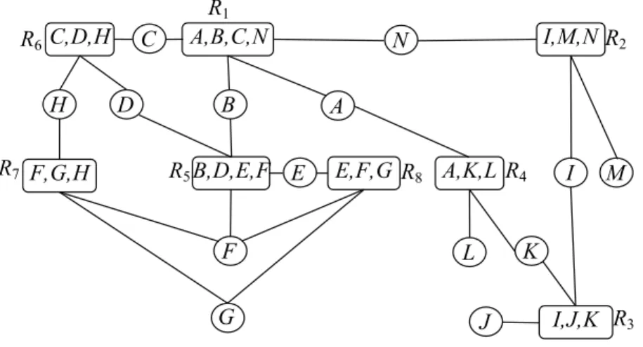
Example 1 Consider the Boolean CSP given by: • X = {A, B, C, D, E, F, G, H, I, J, K, L, M, N }

• D = {DA, DB, DC, DE, DF, DG, DH, DI, DJ, DK, DL, DM, DN}, where each Di = {0, 1}

• C = {hR1, {ABCN }i, hR2, {IM N }i, hR3, {IJ K}i, hR4, {AKL}i, hR5, {BDEF }i,

hR6{CDH}i, hR7, {F GH}i, hR8{EF G}i}

The relations are given in the tables below:

R

₁

A

B

C

N

0

1

0

1

0

1

0

1

0

1

0

1

1 R

₂

I

MN

0

1

0

1

0

1

1 R

₃

I

J

K

0

1

0 R

₄

A

K

L

0

1

0

1

1 R

₅

B

D

E

F

0

1

0

1

0

1

0

1

0 R

₆

C

D

H

0

1

0

1

0 R

₇

F

G

H

0

1

0

1

0 R

₈

E

F

G

0

1

0

1

0

The following variable-value pairs constitute a solution to this CSP:

hA, 0i, hB, 1i, hC, 1i, hD, 0i, hE, 1i, hF, 0i, hG, 0i, hH, 0i, hI, 0i, hJ, 1i, hK, 1i, hL, 0i, hM, 1i, hN, 0i.

(40)

2.1.1 Solving a CSP

Backtrack search is a sound and complete method for finding a solution for a CSP [Bitner and Reingold, 1975]. In this dissertation, we do not use local search because it is not a complete algorithm and may miss a solution even when one exists.

Search operates by assigning a value to a variable and backtracks when a dead-end is encountered by undoing past assignments. The variable-ordering heuristic determines the order that variables are assigned in search, which can be dynamic (i.e., change during search). Boussemart et al.[2004] introduced dom/wdeg, a popular dynamic variable-ordering heuristic. This heuristic associates to each constraint c ∈ C a weight wc(c), initialized to one, that is incremented by one whenever the constraint causes a domain wipeout when enforcing arc consistency. The next variable xi chosen by dom/wdeg is the one with the smallest ratio of current domain size to the weighted degree, αwdeg(xi), given by

αwdeg(xi) =

X

(c∈Cf)∧(xi∈scope(C))

wc(c) (2.1)

where Cf ⊆ C is the set of constraints with at least two future variables (i.e., variables who have not been assigned by search).

Modern solvers enforce a given consistency property on the CSP after each variable assignment. This lookahead removes from the domains of the unassigned variables values that cannot participate in a solution. Such filtering prunes from the search space fruitless subtrees, reducing the size of the search space and thrashing. The higher the consistency level enforced during lookahead, the stronger the pruning and the smaller the search space. A basic form of lookahead is forward checking, which filters the domains of only the unassigned variables connected, by a constraint, to the assigned variable. A more aggressive version of lookahead is Real Full Lookahead

(41)

(RFL) [Nadel, 1989], which enforces a given consistency property on the CSP induced by the unassigned variables (i.e., the future subproblem).

2.1.2 Representation

Several graphical representations of a CSP exist. Below, we introduce five graphical representations:

• In the hypergraph, the vertices represent the variables of the CSP, and the hyper-edges represent the scopes of the constraints. Figure 2.1 shows the hypergraph of the CSP in Example 1. A B C E D F G H I J K M L N R4 R2 R3 R1 R5 R6 R7 R8 Figure 2.1: A hypergraph A B C _E D F G H I J K M L N

Figure 2.2: The primal graph

• In the primal graph, the vertices represent the CSP variables, and the edges con-nect every two variables that appear in the scope of some constraint. Figure 2.2 shows the primal graph of CSP whose hypergraph is shown in Figure 2.1. • The dual graph is the graphical representation of the dual encoding of a CSP.

The dual encoding of a CSP P is a binary CSP, PD_{, where the variables are} the relations of P, and their domains are the tuples of those relations. A constraint exists between two variables in PD if their corresponding relations’ scopes intersect. This constraint enforces the equality of the shared variables. Figure 2.3 shows the dual graph in Figure 2.1.

(42)

R7 R2 R3 R4 R5 R6 R1 A,B,C,N I,J,K I,M,N A,K,L F,G,H B,D,E,F C,D,H N A I K H F B C D R8 E,F,G G,F E,F

Figure 2.3: A dual graph

R7 R2 R3 R4 R5 R6 R1 A,B,C,N I,J,K I,M,N A,K,L F,G,H B,D,E,F C,D,H N A I K H B C D R8 E,F,G G,F E,F

Figure 2.4: A minimal dual graph

• A minimal dual graph of a CSP is its dual graph with no redundant edges are removed. In the dual graph, an edge between two vertices is redundant if there exists an alternate path between the two vertices such that the shared variables appear in every edge in the path [Janssen et al., 1989;Dechter, 2003a]. Redundant edges can be removed without changing the set of solutions. A minimal dual graph can be efficiently computed [Janssen et al., 1989], but is not unique. Figure 2.4 shows a minimal dual graph of Figure 2.3 where the edge linking R5 and R7 is redundant, and thus removed.

• The incidence graph of a CSP is a bipartite graph where one set of vertices contains the variables of the CSP and the other set the constraints. An edge connects a variable and constraint if and only if the variable appears in the scope of the constraint. The incidence graph is the same graph used in the hidden-variable encoding [Rossi et al., 1990]. Figure 2.5 shows the incidence of the CSP of Example 1.

2.1.3 Elimination Ordering and Graph Triangulation

An ordering of a graph is a total ordering of its vertices. The parents of a vertex are the neighbors that appear before it in the ordering. The width of a vertex is the number of its parents. The width of an ordering is the maximum vertex width. The

(43)

E H I J K L M N A B C D F G R1 A,B,C,N R3 I,J,K R2 I,M,N R4 A,K,L R7 F,G,H R5 B,D,E,F R6 C,D,H R8 E,F,G

Figure 2.5: A incidence graph

width of a graph, denoted w, is the minimum width of all its possible orderings, and

can be found in quadratic time in the number of vertices in the graph [Freuder, 1982]. A graph is triangulated, or chordal, iff every cycle of length four or more in the graph has a chord, which is an edge between two non-consecutive vertices. Graph triangulation adds an edge (a chord) between two non-adjacent vertices in every cycle of length four or more. While minimizing the number of edges added by the trian-gulation process is NP-hard, MinFill is an efficient heuristic commonly used for this purpose [Kjærulff, 1990;Dechter, 2003a]. Roughly, MinFill operates by determining, for each vertex, the number of edges needed to fully connect its parents (e.g., number of fill edges). It selects the vertex with the minimum number of fill edges and connects all of its parents. It then repeats until all the vertices have been selected.

A perfect elimination ordering of a graph is an ordering of the vertices such that, for each vertex v, v and the neighbors of v that occur after v in the ordering form a clique. If a graph is triangulated iff the graph has a perfect elimination ordering [Fulkerson and Gross, 1965]. The width of a triangulated graph is called the induced width, denoted w∗, of the ordering used.

2.1.4 Tree Decomposition

A tree decomposition of a CSP is a tree embedding of its constraint network. It is defined by a triple hT , χ, ψi, where T is a tree, and χ and ψ are two functions that

(44)

determine which CSP variables and constraints appear in which nodes of the tree. The tree nodes are clusters of variables and constraints from the CSP. The set of variables of a cluster cl is denoted χ(cl) ⊆ X , and the set of constraints ψ(cl) ⊆ C. A tree decomposition must satisfy two conditions:

1. Each constraint appears in at least one cluster and the variables in its scope must appear in this cluster; and

2. For every variable, the clusters where the variable appears induce a connected subtree.

Many techniques for generating a tree decomposition of a CSP exist [Dechter and Pearl, 1989;Jeavons et al., 1994;Gottlob et al., 2000]. We use here the tree-clustering technique [Dechter and Pearl, 1989].

1. First, we triangulate the primal graph of the CSP using the min-fill heuristic [Kjærulff, 1990].

2. Using the perfect elimination ordering given by the MaxCardinality algo-rithm [Tarjan and Yannakakis, 1984], we identify the maximal cliques in the re-sulting chordal graph using the MaxCliques algorithm [Golumbic, 1980], and use the identified maximal cliques to form the clusters of the tree decomposi-tion. Figure 2.6 shows a triangulated primal graph of the example in Figure 2.1.

The dotted edges (B,H) and (A,I) in Figure 2.6 are fill-in edges generated by the triangulation algorithm. The ten maximal cliques of the triangulated graph are highlighted with ‘blobs.’

(45)

A B C E D F G H I J K M L N C1 C2 C7 C3 C4 C5 C6 C8 C9

Figure 2.6: Triangulated primal graph and its maximal cliques

3. We build the tree by connecting the clusters using the JoinTree algorithm [Dechter, 2003a]. While any cluster can be chosen as the root of the tree, we choose the cluster that minimizes the longest chain from the root to a leaf.

4. Finally, we determine the variables and constraints of each cluster as follows:

a) The variables of a cluster cl, χ(cl), are the variables in the maximal clique

that yields the cluster; and b) The constraints of a cluster cl, ψ(cl), are all the constraints Ri, such that scope(Ri) ⊆ χ(cl). Figure 2.7 shows a tree decompo-sition for the example of Figure 2.1. Note that we may end up with clusters

{A,B,C,N},{R1} {A,I,N},{} {B,C,D,H},{R6} {I,M,N},{R2} {B,D,E,F,H},{R5} C1 C2 C3 C7 C8 {A,I,K},{} C4 {I,J,K},{R3} C5 {A,K,L},{R4} C6 {E,F,G,H},{R7,R8} C9

Figure 2.7: A tree decomposition of the CSP in Figure 2.1

with no constraints (e.g., C2, C4 and C8).

(46)

both clusters.

2.2 Consistency Properties and Algorithms

We distinguish between global and local consistency properties. Algorithms for en-forcing a given consistency property typically operate by filtering values from the variables’ domains or tuples from the constraints’ relations. For any consistency property, there could be a number of algorithms for enforcing it on a CSP.

Global consistency properties are defined over the entire CSP. Minimality and

decomposability are two global consistency properties [Montanari, 1974]. Constraint minimality requires that every tuple in a constraint appears in a solution. Decompos-ability guarantees that every consistent partial solution of any length can be extended to a complete solution. Decomposability is a highly desirable property: it guaran-tees that the CSP can be solved in a backtrack-free manner. Because guaranteeing a globally consistent CSP is in general exponential in time and space [Bessiere, 2006], we focus in practice on local consistency properties, which are in general tractable.

Local consistency properties are defined over combinations of a fixed size of

vari-ables (i.e., variable-based consistency) or constraints (i.e., relation-based consistency). A local consistency property guarantees that the values of all combinations of a given number of CSP variables (alternatively, the tuples of all combinations of a given size of CSP relations) are consistent with the constraints that apply to them. This con-dition is necessary but not sufficient for the values (or the tuples) to appear in a solution to the CSP.

Below, we review the main variable-based and relation-based consistency proper-ties relevant to this dissertation.

(47)

2.2.1 Variable-Based Consistency

The most common property is Arc Consistency (AC) for binary CSPs, or Generalized Arc Consistency (GAC) for non-binary CSPs [Mackworth, 1977].

Definition 1 Generalized Arc Consistent (GAC) [Mackworth, 1977]: A CSP is

Gen-eralized Arc Consistent (GAC) iff, for every constraint ci, and every variable x ∈ scope(ci), every value v ∈ dom(x) is consistent with ci (i.e., appears in some consis-tent tuple of Ri).

Algorithms for enforcing GAC remove domain values that have no GAC-support, leaving the relations unchanged [Bessière et al., 2005]. Simple Tabular Reduction (STR) algorithms not only enforce GAC on the domains, but also remove all tuples

τ ∈ Rj where ∃xi ∈ scope(Rj) such that τ [xi] /∈ dom(xi) [Ullmann, 2007; Lecoutre,

2011; Lecoutre et al., 2012].

Definition 2 Max Restricted Path Consistent (maxRPC) [Debruyne and Bessière, 1997a]: A binary CSP is max Restricted Path Consistent (maxRPC) iff it is (1,

1)-consistent and for all xi ∈ X , for all a ∈ dom(xi), for all xj ∈ X s.t. there exists c ∈ C with scope(c) = {xi, xj}, there exists b in dom(xj), s.t. for all xl ∈ X , there exists d ∈ dom(xl) s.t. the 3-tuple ((xi, a), (xj, b), (xl, d)) is consistent.

Informally, a problem is maxRPC iff it is (1, 1)-consistent and for each value (xi, a) and variable xj linked to xi by some constraint, there is a consistent extension b of a on xj and this pair of values is path consistent.1

An extension of maxRPC to non-binary CSPs is maxRPWC.

Definition 3 max Restricted Pairwise Consistent (maxRPWC) [Bessière et al., 2008]:

A CSP is max Restricted Pairwise Consistent (maxRPWC) iff ∀xi ∈ X and ∀a ∈

(48)

dom(xi), ∀cj ∈ C, where xi ∈ scope(cj), ∃τ ∈ rel(cj) such that τ [xi] = a, τ is valid, and ∀cl ∈ C(cl 6= cj), s.t. scope(cj) ∩ scope(cl) 6= ∅, ∃τ /∈ rel(cl), s.t. τ [scope(cj) ∩ scope(cl)] = τ0[scope(cj) ∪ scope(cl)] and τ0 is valid. In this case we say that τ0 is a PW-support of τ .

Singleton Arc-Consistency (SAC) ensures that no domain becomes empty when enforcing GAC after assigning a value to a variable [Debruyne and Bessière, 1997b]. This operation is called a singleton test. Let GAC(P ∪ {xi ← vi}) be the CSP after assigning xi ← vi and running GAC.

Definition 4 Singleton Arc-Consistency (SAC) [Debruyne and Bessière, 1997b]: A

variable-value pair (xi, vi) of the CSP P is Singleton Arc-Consistency (SAC) iff GAC(P ∪ {xi ← vi}) 6= ∅ (the singleton check). P is SAC iff every variable-value pair is SAC.

Algorithms for enforcing SAC remove all domain values that fail the singleton test. Neighborhood SAC (NSAC) [Wallace, 2015] restrict the AC check of SAC to the neighborhood of a variable. Given a CSP P and V a subset of the variables of P, we denote P|V the subproblem induced by V on P. The constraints included in P|V are

all those constraints whose scope contains a variable in V.

Definition 5 Neighborhood Singleton Arc-Consistency (NSAC) [Wallace, 2015]: A

variable-value pair (xi, vi) of the CSP P is Neighborhood Singleton Arc-Consistency (NSAC) iff GAC(P|{xi}∪neigh(xi)∪ {xi ← vi}) 6= ∅ (the singleton check). P is NSAC

iff every variable-value pair is SAC.

Partition-One Arc-Consistency (POAC) adds an additional condition to SAC [Bennaceur and Affane, 2001]. Let (xi, vi) denote a variable-value pair, (xi, vi) ∈ P iff vi ∈ dom(xi).

(49)

Definition 6 Partition-One Arc-Consistent (POAC) [Bennaceur and Affane, 2001]:

A constraint network P = (X , D, C) is Partition-One Arc-Consistent (POAC) iff P is SAC and for all xi ∈ X , for all vi ∈ dom(xi), for all xj ∈ X, there exists vj ∈ dom(xj) such that (xi, vi) ∈ GAC(P ∪ {xj ← vj}).

Balafrej et al. [2014] introduced two algorithms for enforcing POAC: POAC-1 and its adaptive version APOAC.

1. POAC-1 operates by enforcing SAC. In POAC-1, all the CSP variables are singleton tested and the process is repeated over all the variables until a fixpoint is reached. When running a singleton test on each of the values in the domain of a given variable, POAC-1 maintains a counter for each value in the domain of the remaining variables to determine whether or not the corresponding value was removed by any of the singleton tests. Values that are removed by each of those singleton tests are identified as not POAC and removed from their respective domains. POAC-1 typically reaches quiescence faster than SAC. 2. In APOAC, the adaptive version of POAC-1, the process is interrupted as soon

as a given number of variables is processed. This number depends on input parameters and is updated by learning during search.

Neighborhood Inverse Consistency (NIC) [Freuder and Elfe, 1996] ensures that every value in the domain of a variable xi can be extended to a solution of the subproblem induced by xi and the variables in its neighborhood.

Definition 7 Neighborhood Inverse Consistency (NIC) [Freuder and Elfe, 1996]: A

variable xi is Neighborhood Inverse Consistency (NIC) iff every value in dom(xi) can be extended to the variables in neigh(xi) that satisfies all the constraints in neigh(xi). A network is NIC iff every variable is NIC.

(50)

2.2.2 Relation-Based Consistency

In the dual graph of a CSP, the vertices represent the CSP constraints and the edges connect vertices representing constraints whose scopes overlap. Relational Neighbor-hood Inverse Consistency (RNIC) [Woodward et al., 2011b] enforces NIC on the dual graph of the CSP. That is, it ensures that any tuple in any relation can be extended in a consistent assignment to all the relations in its neighborhood in the dual graph. Definition 8 Relational Neighborhood Inverse Consistent (RNIC) [Woodward et al., 2011b]: A relation Ri is Relational Neighborhood Inverse Consistent (RNIC) iff every tuple in Ri can be extended to the variables in SRj∈Neigh(Ri)scope(Rj) \ scope(Ri) in

an assignment that simultaneously satisfies all the relations in Neigh(Ri). A network is RNIC iff every relation is RNIC.

NIC and RNIC are theoretically incomparable [Woodward et al., 2012], but RNIC has two main advantages over NIC:

1. NIC was originally proposed for binary CSPs and the neighborhoods in NIC likely grow too large on non-binary CSPs.

2. RNIC can operate on different dual graph structures to save time and/or im-prove propagation. Three variations of RNIC were introduced and operate on dual graphs that are minimal (wRNIC), triangulated (triRNIC), or both min-imal and triangulated (wtriRNIC) [Woodward et al., 2011a; Woodward et al., 2011c]. Given an instance, selRNIC uses a decision tree to automatically select the dual graph for RNIC to operate on.

Definition 9 m-wise consistent [Gyssens, 1986; Janssen et al., 1989]: A CSP is

m-wise consistent if, every tuple in a relation can be extended to every combination of m − 1 other relations in a consistent manner.

(51)

Pairwise Consistency (PWC) guarantees that every tuple consistent with a constraint

ci is consistent with every constraint in neigh(ci) [Gyssens, 1986]. Pairwise Consis-tency is equivalent to 2-wise consisConsis-tency. Keeping with relational-consisConsis-tency nota-tions, Karakashian et al. denoted m-wise consistency by R(∗,m)C, and proposed a first practical algorithm for enforcing it [2010]. For simplicity, we will refer to R(∗,m)C as the property combining both GAC and R(∗,m)C, which can be obtained algorithmically by projecting the relations onto their scopes individually after enforc-ing R(∗,m)C.

Montanari [1974] originally introduced the property of path consistency as a tractable approximation of minimality.

Definition 10 Path Consistent (PC) [Dechter, 2003a]: Given a CSP P, the variables

xi and xj are Path Consistent (PC) relative to a variable xk6=i for every consistent assignment {(xi, a), (xj, b)} there is some value c ∈ dom(xk) such that both the as-signments {(xi, a), (xk, c)} and {(xj, b), (xk, c)} are consistent. P is path consistent iff ∀xi, xj, xk∈ V with xk 6= xi 6= xj, xi and xj are path consistent relative to xk.

Directional path consistency (DPC) is a restriction of path consistency to an ordering ord of the variables, typically the perfect elimination ordering.

Definition 11 Directional Path Consistent (DPC) [Dechter and Pearl, 1988]: A CSP

is Directional Path Consistent (DPC) relative to order ord = (x1, x2. . . , xn), iff for every k ≥ i, j, the two variables xi and xj are path consistent relative to xk.

Conservative Path Consistency (CPC) is a restriction of path consistency to the existing constraints of a problem. If there is no Ci,j ∈ C then xiand xjare conservative path consistent, otherwise xi and xj must be path consistent.

(52)

Definition 12 Conservative Path Consistent (CPC) [Debruyne, 1999]: An

assign-ment to two variables xi and xj such that there is no constraint Ci,j ∈ C is Conserva-tive Path Consistent (CPC). If Ci,j ∈ C, the assignment {(xi, a), (xj, b)} is conserva-tive path consistent iff (a, b) ∈ Ri,j and ∀xi, xj, xk ∈ V with k 6= i 6= j, Ci,k, Cj,k ∈ C ⇒ ∃c ∈ dom(xk) such that (a, c) ∈ Ri,k and (b, c) ∈ Rj,k. A constraint Ci,j ∈ C is conser-vative path consistent iff for all the tuples (a, b) ∈ Ri,j, the assignment {(xi, a), (xj, b)} is conservative path consistent. A CSP is conservative path consistent iff it is arc con-sistent and ∀Ci,j ∈ C, Ci,j is conservative path consistent.

Partial path consistency [Bliek and Sam-Haroud, 1999] was introduced in the same year as CPC. We present the definition as phrased by Lecoutre et al. [2011].

Definition 13 Partial Path Consistent (PPC) [Lecoutre et al., 2011]: A CSP is

Partial Path Consistent (PPC) iff every closed graph-path of its constraint graph is consistent.

The algorithms for enforcing PPC on a CSP involves triangulating the CSP (i.e., generating constraints for the added triangulated edges) and enforcing CPC on the triangulated network.

Definition 14 Conservative Dual Consistent (CDC) [Lecoutre et al., 2007]: Given

a CSP, P, an assignment {(xi, a), (xj, b)} is Conservative Dual Consistent (CDC) iff (ci,j ∈ C) ∨ ((x/ j, b) ∈ AC(P|xi←a) ∧ (xi, a) ∈ AC(P|xj←b)). P is conservative

dual consistent iff every consistent assignment {(xi, a), (xj, b)} is conservative dual consistent.

Higher-Level Consistencies : When, Where, and How Much

HAL Id: tel-02295985

https://tel.archives-ouvertes.fr/tel-02295985

Much

Robert J. Woodward

To cite this version:

RAPPORT DE GESTION

2015

THÈSE POUR OBTENIR LE GRADE DE DOCTEUR

DE L’UNIVERSITÉ DE MONTPELLIER

Présentée par Robert J. WOODWARD

Le 20 septembre 2018

Sous la direction de Christian BESSIERE

et Berthe Y. CHOUEIRY

Les Cohérences Fortes : Où, Quand, et Combien

Contents

List of Figures

List of Tables

Chapter 1

Introduction

1.1

Motivation and Claims

Where?

When?

How much?

HLC

Where?

When?

How much?

1.2

Approach

1.2.1

Visualizing Search and Consistency Costs

APOAC

#BTs

CPU Time: 23.77 sec.

#NV: 59,181

#BT: 53,212

#Calls POAC: 11,142

APOAC

#BTs

Filter

No Filter

Wipeout

CPU Time: 23.77 sec.

#NV: 59,181

#BT: 53,212

#Calls POAC: 11,142

1.2.2

‘When:’ Reactive Strategies for Enforcing HLC

1.2.3

‘How Much:’ Monitoring Constraint Propagation

1.2.4

‘Where:’ Channel HLC along Cycles

1.3

Contributions

1.4

Outline of Dissertation

Summary

Chapter 2

Background

2.1

Constraint Satisfaction Problem (CSP)

R

A

B

C

N

0

0

0

1

0

1

0

1

0

1

1

0

_#BTs