Annabi: HEC Montréal
Breton: HEC Montréal and GERAD. Correspondence to: Michèle Breton, HEC Montréal, 3000 Côte-Sainte-Catherine, Montréal (QC), Canada H3T 2A7
François: HEC Montréal and CIRPÉE
We would like to thank Jan Ericsson, Jean Helwege and Franck Moraux for their useful comments. We also thank Ali Boudhina for excellent research assistance. Annabi and Breton acknowledge financial support from IFM2 and
Cahier de recherche/Working Paper 10-48
Resolution of Financial Distress under Chapter 11
Amira Annabi
Michèle Breton
Pascal François
Abstract:
We develop a contingent claims model of a firm in financial distress with a formal
account for renegotiations under the Chapter 11 bankruptcy procedure. Shareholders
and two classes of creditors (senior and junior) alternatively propose a reorganization
plan subject to a vote. The bankruptcy judge can intervene in any renegotiation round to
impose a plan. The multiple-stage bargaining process is solved in a non-cooperative
game theory setting. The calibrated model yields liquidation rate, Chapter 11 duration
and percentage of deviations from the Absolute Priority Rule that are consistent with
empirical evidence.
Keywords: Credit risk, Chapter 11, game theory, dynamic programming
1
Introduction
A corporation in …nancial distress can either negotiate privately with its claimants or …le under the protection of the legal bankruptcy procedure. The recent bailouts of some major U.S. companies during the latest crisis has emphasized the complex and critical impact that the bankruptcy procedure can have on the economy as a whole. In the U.S., Chapter 11 of the bankruptcy Code presents an alternative to the liquidation of a bankrupt …rm by de…ning a judicial context in which the …rm can reorganize its activities in order to emerge as a viable entity. Over the last few years, Chapter 11 has become the dominant mode of resolution of …nancial distress for large public companies. Among the 213 bond defaults recorded by Moody’s from 1997 to 2005, Davydenko (2010) documents that 54% of them are technical defaults (i.e. missed payment), while 37% are resolved through Chapter 11, with only 9% of defaults being resolved out of Court. These …gures highlight the need for a better understanding of the bankruptcy mechanism.
The aim of this paper is to formally model the characteristics of Chapter 11 negotia-tion and to analyze the determinants of reorganizanegotia-tion outcomes. Speci…cally, we model the strategic interaction between claimants in Chapter 11 as a multiple-stage bargaining process, and solve it in a non-cooperative game theory setting. Our paper adds to the earlier literature by modeling a complex and realistic negotiation process, that incorporates di¤er-ent features of Chapter 11. In particular, we consider two classes of creditors with di¤erdi¤er-ent seniorities and allow claimants to sequentially propose reorganization plans. Shareholders bene…t from the exclusivity period that allows them to propose the …rst plan. One of these plans can be con…rmed by the bankruptcy judge if all claimants agree on its implementa-tion. We also account for Chapter 11 cramdown provision which allows the judge to impose a reorganization plan, thereby putting an end to a lengthy and costly negotiation. Further-more, the bankruptcy judge has the opportunity to impose her own reorganization plan. Finally, our model respects the rule of automatic stay of assets as creditors are not allowed to liquidate parts of the assets as negotiations move from one round to another.
equi-libria (liquidation, reorganization, or continuation to the next round) for every possible asset value. By specifying a standard di¤usion process for asset value, we associate a prob-ability to each of these equilibria, which yields a probabilistic representation of the Chapter 11 procedure with formal bargaining.
In line with empirical evidence, our model can generate several rounds of bargaining. Ongoing negotiations are driven by claimholders’ uncertainty about judge behavior. De-pending on …rm asset value, the class of claimants, which proposes a reorganization plan, can have an incentive to narrow the chances of unanimous acceptance and hope for the judge to impose terms that are more favorable to them.
Once the model is calibrated on characteristics of …rms entering Chapter 11 as well as on the bankruptcy timeline and costs, it replicates stylized facts about liquidation rates, time spent under Chapter 11, and frequency of deviations from the Absolute Priority Rule (APR).
The remainder of the paper is organized as follows. After a brief review of the related literature in section 2, we formally introduce the negotiation process under Chapter 11 in section 3. In section 4, we solve the game by backward induction and characterize the possible equilibrium outcomes. Section 5 presents the data and calibration method used to implement the model numerically. Model results are analyzed and compared to empirical evidence in section 6. Section 7 concludes.
2
Related literature
Early contingent claims models of corporate debt assimilate default with immediate liq-uidation (Merton, 1974, Leland, 1994). The modelling of …nancial distress has primarily focused on out-of-Court renegotiations. Anderson and Sundaresan (1996) and Mella-Barral and Perraudin (1997) analyze strategic debt service, i.e. coupon reductions that sharehold-ers can impose to creditors every time the …rm is close to default. Mella-Barral (1999) study private debt renegotiations when shareholders and creditors can alternatively make take-it-or-leave-it o¤ers. Fan and Sundaresan (2000) view renegotiations as a cooperative Nash
bargaining game in which claimholders maximize renegotiations surplus to avoid costly liq-uidation. However, the assumption of a cooperative game for renegotiations may be harder to sustain for Chapter 11. Indeed, Brown (1989) and Gertner and Scharfstein (1991) argue that …rms in default will cease private renegotiations and …le bankruptcy when hold out problems are severe. Gilson, John and Lang (1990) as well as Datta and Iskandar-Datta (1995) provide empirical support for this view.
Bruche and Naqvi (2010) explicitly account for an agency con‡ict during …nancial dis-tress between shareholders and creditors, as the former decide on the time to default while the latter decide on the time to liquidate. As acknowledged by these authors, this frame-work is best suited for creditor-friendly bankruptcy procedures. In Chapter 11, the judge is in‡uential in preserving the going-concern value of the …rm.
Hege and Mella-Barral (2005) and Hackbarth, Hennessy and Leland (2007) enrich the renegotiation framework by allowing for multiple creditors. Both works examine exchange o¤ers proposed by shareholders. In Hackbarth, Hennessy and Leland (2007), one class of debt is bank debt and assumed to be renegotiable. The other is market debt, cannot be renegotiated, but allows the …rm to increase its debt capacity.
More recent are the contributions which aim at capturing Chapter 11 speci…city into the modelling of …nancial distress. Moraux (2002), François and Morellec (2004), Galai, Raviv and Wiener (2007), and Broadie, Chernov and Sundaresan (2007) assume that liquidation after Chapter 11 is triggered by the excursion of asset value beneath a default threshold. In these works however, the role of the judge is not taken into account. But, as documented by Chang and Schoar (2008), the in‡uence of the judge on Chapter 11 outcomes is far from neutral.
From a di¤erent methodological standpoint, various classi…cation models have been applied to the bankruptcy procedure. For instance, Luther (1998) uses arti…cial neural networks to predict Chapter 11 outcome. These works relate the likelihood of liquidation vs. reorganization to the …nancials of defaulting …rms, but again, they fail to acknowledge procedural aspects (including the role of the judge) as a key determinant of corporate
restructuring.
3
The negotiation process model under Chapter 11
Our modelling needs to be consistent with the main features of the Chapter 11 procedure. In the vast majority of cases, the …rm in default …les under Chapter 11 on a voluntary basis (see e.g. White, 1996, for evidence). As a result, the management team stays in place after …ling, and enjoys an exclusivity period during which it can propose the …rst reorganization plan.1 Acceptance of the plan is subject to a vote among classes of claimholders. The judge observes the process and can either validate the plan if unanimously accepted, call for another round of renegotiations if unanimous consent is not achieved, or pronounce …rm liquidation if reaching an agreement becomes unlikely. The judge may also use the cramdown provision, which allows her to impose a reorganization plan when she believes the procedure is getting too lengthy and costly.2 In practice, successfully reorganized …rms may need more than one reorganization plan (see e.g. Carapeto, 2005).
Shareholders and creditors bargain over a sharing rule for asset value. The rule of automatic stay prevents creditors to seize assets during renegotiations. Hence the dynamics of asset value is not subject to partial liquidations (also known as "asset stripping").3 We assume that all claimants have the same information about asset value, characteristics of bankruptcy procedure and judge behaviour. In spite of bargaining being costly, we show that our perfect and complete information setting can generate more than one round of renegotiations. This is because claimholders are unsure about the judge behaviour, and assign probabilities about her intervention in the negotiation process. In contrast to Giammarino (1989) who argues that informational asymmetries increase the number
1
This …rst plan is in the best interests of shareholders as we abstract from agency con‡icts between claimants.
2Berkovitch, Israel and Zender (1998) show that judge interference in the procedure is a direct restriction
on the bargaining game that prevents claimholders from acting too strategically.
3
One exceptional case of asset stripping is the failure of Eastern Airlines documented by Weiss and Wruck (1998).
of bargaining rounds and may require the intervention of the Court, we show that even homogenous information among claimholders can generate multiple round bargaining as soon as the judge behavior is perceived as uncertain.
3.1 The …rm
We consider a …rm …nanced by two classes of debt with di¤erent priorities, paying a constant and continuous coupon c to the creditors, and a constant dividend to the equityholders, until default. We denote by Vt the the value of the …rm’s assets at time t and assume that Vt, which plays the role of a state variable, is instantly observable by all players. The default event, at t = 0, starts the negotiation process under Chapter 11. We assume that coupon and dividend payments are suspended during Chapter 11 negotiation, and resume if and once the …rm emerges from the process as a reorganized entity, at date t : The …rm’s assets value then follows a regime-switching log-normal process under the risk neutral measure:
dVt= 8 < : rVtdt + VtdZt if 0 t < t (r ) Vtdt + VtdZt if t t < T (1)
where r denotes the risk-free rate, the dividend payout rate, the volatility of the assets, Ztis a Q Brownian motion and T is a stopping time representing the eventually reorganized …rm default event date.
3.2 The players
The negotiation process under Chapter 11 involves all the claimants of the …rm, as well as the bankruptcy judge. The creditors and equityholders are strategic participants, having a stake in the …rm, while the bankruptcy judge is a non-strategic player.
We assume the interests of the equityholders are represented by the same board of directors as prior to …ling and identify it with a single player, denoted Player e. The creditors are divided into two classes of substantially similar claims, labeled senior and junior (subordinated). As provided in the Code, the bankruptcy judge appoints a committee to represent the interests of creditors in each class during the reorganization. We identify
single players, denoted respectively by s and j, with the negotiators representing the interest of senior and junior creditors. During the negotiation process, strategic players e; s and j take their decisions independently, by taking into account their best individual interest.
Empirical evidence suggests that the bankruptcy judge, while having no personal stake in the negotiation, does in‡uence the negotiation by controlling key parameters of the process. Here, we let the judge decide on the maximum number of negotiation rounds, denoted K, and allow her to intervene and stop the process at any round if an agreement is not reached among the strategic players. The probability of the judge’s intervention at round k; denoted by qk, re‡ects the impatience of the judge, and can, for instance, increase with the number of bargaining rounds and/or the length of the negotiation process.
Conditional on intervening, we further assume that the judge can either cramdown a reorganization plan, or convert Chapter 11 negotiation into Chapter 7 liquidation.4 In the event of a cramdown, the judge can decide to impose the last proposed plan, or any other reorganization plan she …nds "fair and equitable". What the judge will decide is not known with certainty, and we denote by z the probability that the judge imposes her own plan. A parameter, denoted , describes the judge’s attitude towards the claimants, that is, the relative weight allocated to them in her own reorganization plan. The judge’s behavior is thus characterized by the parameters K, qk, z, and , which we assume known by all the claimants at the beginning of the negotiation process.
3.3 Bankruptcy costs
Bankruptcy costs are divided into two categories: …nancial distress costs are borne during the negotiation process, while liquidation costs reduce the value recovered from the assets in the case of a liquidation. Bankruptcy costs play an important role, making a prompt negotiated outcome interesting for all parties.
4To liquidate the …rm, the bankruptcy judge can invoke one of the causes described in section 1112(b)(4)
of the Bankruptcy Code. For example, showing that there is substantial or continuing loss to the estate and the absence of a reasonable likelihood of rehabilitation. Other causes can include some negotiation technicalities.
We model …nancial distress costs that are proportional both to the value of the assets at the beginning of Chapter 11 negotiation, and to the length of the negotiation process, capturing elements of direct (legal fees) as well as indirect (productivity loss) costs. For simplicity, we assume that all bargaining rounds are of equal length d. Accordingly, an amount V0d is due (in priority) at the end of each bargaining round, thus reducing the total value of the shares of the claimants in the reorganized …rm. In order to keep track of the cumulated value of the …nancial distress costs, capitalized at rate r, at the end of negotiation round k, de…ne
Ck = Xk 1 j=0 1 + e rdj V 0d = 1 e rdk 1 erd V0d. (2)
On the other hand, liquidation costs are assumed to be proportional to the …rm’s remain-ing asset value, net of …nancial distress costs. The proportion of the ex-…nancial distress costs asset value recovered in the case of a liquidation is denoted by 1 .
3.4 Chapter 11 outcomes
According to the provisions of the Code, each negotiation round consists in the proposal of a reorganization plan by one of the player to the other claimants, who then vote to accept or reject it. Thus, at each negotiation round, a plan is submitted by one of the players, labeled Leader, to the two other players, labeled Follower 1 and Follower 2. We consider three possible outcomes, depending on the followers’reaction to the leader’s proposition.
In the …rst case, the …rm is reorganized and emerges as a new entity. This new …rm is shared between the claimants either according to the plan proposed by the leader at that round (if the followers agreed to it, or if the judge imposed it), or according to a plan decided by the judge. In the second case, the …rm is liquidated. This happens if the judge decides to stop the negotiation process when the plan proposed by the leader is unanimously rejected by the two followers. Finally, in the third case, nothing is resolved and the process moves to the next negotiation round, where another player is selected to propose a new
reorganization plan. This happens if the judge does not interfere in the bargaining process when the followers do not accept the leader’s proposition. However, since …nancial distress costs are borne continuously during the negotiation process, whenever the …rm’s assets value is no longer su¢ cient to cover the cumulated …nancial distress costs, then the reorganization process stops and the …rm is immediately liquidated under Chapter 7 of the Code, leaving nothing to the claimants.
4
Solving the negotiation game
In this section, we solve for the equilibrium strategies of the three strategic players, and obtain, for each player, the expected value of the outcome of the negotiation game, at the moment the default event is triggered.
4.1 Time sequence of events
Our model spans the life of the …rm, over an in…nite horizon, starting from t = 0 when a default event triggers the Chapter 11 negotiation process. If the process results in a reorganization, at date t , the reorganized …rm continues operating until a second default event occurs at date T .
We assume that the …nancial distress costs are covered by the …rm’s asset during the negotiation process. The …rm stops operating, with a null recovery value, if at any time during the negotiation the value of the assets vanishes.
At t = 0, coupon and dividend payments are suspended. The equityholder then has d units of time to prepare a …rst reorganization plan to be submitted to the creditors.
At t = d, provided Vd > C1; the …rst plan is proposed. If both creditors approve the plan, or if the judge intervenes with a cram-down, a new reorganized …rm emerges; this …rm distributes dividends and new reorganized coupons, and continues its operations until T . If the judge intervenes and imposes liquidation, the …rm is liquidated according to the Absolute Priority Rule and the process terminates. Otherwise, the negotiation process
continues: the junior creditor has d units of time to prepare a second reorganization plan to be submitted to the two other claimants, namely the equityholder and the senior creditor. At t = 2d, provided V2d> C2; the second plan is proposed. Again, the …rm may emerge if both players approve the plan, or if the judge cramdowns a plan, or may be liquidated if the judge so decides. Otherwise, the senior creditor has d units of time to prepare a third reorganization plan to be submitted to the two other claimants.
At t = 3d, provided V3d > C3; the third plan is proposed, with the three same possible outcomes. If the process continues, the claimants alternate in proposing reorganization plans following the same sequence, until either the …rm is reorganized or liquidated.
For simplicity and tractability reasons, we assume that any further …nancial distress after the …rm emerges from Chapter 11 leads to the liquidation of the …rm.
4.2 Outcome values
In our setting, the players strategies and the resulting Chapter 11 outcomes depend on the observed level of the assets value, which de…nes the state of the system, and on the initial debt contract, represented here by the contractual coupons, which are given parameters. We denote the contractual coupons by c0= c0s+ c0j; where c0s is the senior debt coupon and c0
j is the subordinated debt coupon. In the following subsections, we compute the value of what each claimant receives according to the outcome of the negotiation process, at discrete times t = kd corresponding to the end of the kth negotiation round. To keep track of the value of assets net of …nancial distress costs at date t = kd when v = Vkd, we de…ne the auxiliary variable wk v Ck.
4.2.1 Liquidation
If the …rm is liquidated after k negotiation rounds at time t = kd, the assets of the …rm, net of the …nancial distress costs, are disposed of at a proportional liquidation costs . The liquidation value of the …rm thus depends on the asset value v = Vkd and on the cumulated
…nancial distress costs at the end of round k, and is given by:
!LF(v; k) = max [(1 ) wk; 0] . (3)
If wk 0, then nothing is left to be shared among the claimants and !LF(v; k) = 0. How-ever, if wk > 0, then the senior, junior and equityholders liquidation payo¤s, according to Absolute Priority Rule, depend on the contractual coupons c0s and c0j, and are given respectively by !Ls(v; k) = min !LF(v; k);c 0 s r ; (4) !Lj(v; k) = min " max !LF(v; k) c 0 s r; 0 ; c0j r # ; (5) and !Le(v; k) = max !LF(v; k) c 0 r; 0 : (6) We denote by !L(v; k) = !L
s( ); !Lj( ); !Le( ) the vector of liquidation values at assets value v and negotiation round k:
4.2.2 Emergence values
If the …rm emerges from …nancial distress after k negotiation rounds at time t = kd and asset value v = Vt Ck > 0, then the reorganized …rm continues its operations by distributing new coupons cs and cj to the senior and junior creditors respectively, until further default at time T . Recall that we assume that further default leads to immediate liquidation. The value at (v; k) of the reorganized …rm depends on the reorganized coupon and on the value of the assets, net of …nancial distress costs, at the emergence from Chapter 11, and is given by: Evt Z T t ( c + Vu) e r(u t)du + (1 )Evt h e r(T t)Bi (7)
where Evt( ) denotes the expectation EQ( jt; Vt= v) under the risk-neutral measure Q, represents the tax rate, c cs+ cj is the total reorganized coupon, the payout rate, r the risk-free interest rate, the proportional liquidation costs and B the …nal default barrier.
Equivalently, the value of the …rm after emergence, which is the object of bargaining between claimants, is given by:
!RF(v; c; k) = wk+ c r 1 B wk 1 ! B B wk 1 (8) where = + ++ , = r 2 2
and = p2r + 2. The …rst term in (8) is the value of the assets at the emergence time, the second term is the present value of tax bene…ts of the operating …rm, and the third term is the present value of liquidation costs.
Denote the liquidation values for each claimant at the …nal default barrier B when the reorganized coupon pair is c (cs; cj) by !Di (B; c); i 2 fs; j; eg. Upon reorganization at (v; k) with a new coupon c = cs+ cj, the value for the three claimants (senior creditor, junior creditor and equityholder) is therefore given respectively, for v > Ck; by
!Ri (v; c; k) = ci r 1 B wk 1 ! + !Di (B; c) B wk 1 ; i 2 fs; jg (9) and !Re (v; c; k) = !RF(v; c; k) !Rs (v; c; k) + !Rj (v; c; k) = wk (1 ) c r 1 B wk 1 ! B B wk 1 + !De (B; c): (10) Following Leland (1994), we assume that default is decided by equityholders, and that the liquidation barrier B is determined so as to maximize equity value, given the limited liability of equityholders. The optimal liquidation barrier for equityholders is then
B = (1 )
r c. (11)
Notice that the reorganized coupon c has a direct impact on the liquidation barrier. Using the expression of the default barrier in (11) and rearranging (8), the total value of the …rm at v; k when the reorganized coupon is c for v > Ck is given by:
!RF(v; c; k) = wk + c rwk 1 + (1 ) c rwk 1 1 ! (12)
As developed by Leland (1994), the liquidation leaves the creditors with value (1 ) B and the equityholders with nothing. Rearranging (9), the total value of debt for v > Ck is given by !Rs (v; c; k) + !Rj (v; c; k) = wk c rwk 1 1 (1 ) (1 ) c rwk 1 1 ! ; (13)
while the value of equity for v > Ck is !Re (v; c; k) = wk (1 ) c rwk + (1 ) (1 ) c rwk 1 1 ! : (14)
Notice that, at a given time kd and asset value v, both the value of the reorganized …rm and of the reorganized debt are concave in c, while the value of equity is decreasing in c.
We denote by !R(v; c; k) = !Rs( ); !Rj( ); !Re( ) the vector of reorganization values at asset value v, negotiation round k and when the reorganized coupon pair is c.
4.2.3 The role of the judge
A reorganized …rm may emerge from …nancial distress after k negotiation rounds at time t = kd and asset value v = Vt under the bankruptcy judge’s plan. We suppose that the judge’s plan is, as stipulated in the Code, fair and equitable; in that respect, we assume that the judge’s plan gives to each player at least his liquidation payo¤, thus ruling out Absolute Priority Rule violation, and shares the residual value among the claimants according to some sharing vector, denoted by = s; j; e ; satisfying:
0 i 1; i 2 fs; j; eg and
X i2fs;j;eg
Therefore, a reorganized coupon pair proposed by the bankruptcy judge, denoted c , is such that the each claimant’s payo¤ satis…es
!Ri (v; c ; k) = i !RF(v; c ; k) !LF(v; k)
| {z }
Residual value
+ !Li(v; k), i 2 fs; j; eg (15)
where !R
F(v; c ; k) is the total …rm value de…ned in (12) and the liquidation payo¤s !Li(v; k) are de…ned in (4) (6) for i 2 fs; j; eg. For a given (v; k), the reorganized coupon pair satisfying (15) is denoted by c to simplify notation - but is a function of (v; k) (see Appendix A). The sharing vector de…nes the proportion of the "bene…ts of reorganization" that each player gets from the judge’s plan. This can be assimilated to the solution of a Nash bargaining game, where would then represent the vector of the claimant’s bargaining powers, the residual value corresponding to the bene…t of cooperation between the claimants, and where the liquidation payo¤s represent the non-cooperation threat.
4.2.4 Continuation values
If the …rm is neither reorganized, nor liquidated after k negotiation rounds, then we de…ne continuation values at time t = kd and state variable value v = Vt, which are the expected values of the players future payo¤s, taking into account the dynamics of the …rm’s asset value.
Denote ! (v; k) = !s( ) ; !j( ) ; !e( ) the vector of equilibrium outcomes of nego-tiation round k when the …rms’ assets value Vkd = v, k 2 [1; K], that is, for a claimant i 2 fs; j; eg: !i (v; k) = 8 > > > > > > > > > < > > > > > > > > > : 0 if v Ck !Li (v; k) if the …rm is liquidated !R
i (v; c; k) if the …rm is reorganized with c !Ci (v; k) otherwise 9 > > > = > > > ; if v > Ck (16)
where the continuation payo¤ !Ci (v; k) for each player is de…ned as the expected value of the outcome at the next bargaining round, and continuation is not allowed when the game
reaches the end of the negotiation process, such that, for i 2 fs; j; eg ; !Ci (v; k) = 8 < : e rdEvt ! V(k+1)d,k + 1 for k = 0; : : : ; K 1 0 for k = K: (17)
We denote by !C(v; k) = !Cs ( ) ; !Cj (v; k) ; !Ce (v; k) the vector of continuation outcomes at (v; k) and !C
F (v; k) = !Cs (v; k) + !Cj (v; k) + !Ce (v; k) the continuation value of the …rm at (v; k), k 2 [0; K] :
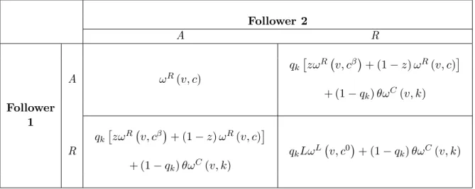
4.3 Negotiation round game
Table 1 depicts the normal form representation of the game at a given round k, between the claimant who proposes a reorganization plan, labelled 0 for "Leader", and the other two claimants, labelled 1 and 2 for "Follower 1" and "Follower 2", who vote on it. Notice that we use numerical labels when the claimants are referred by their role as players in the negotiation process, i = f0; 1; 2g, and literary labels when they are identi…ed by their role as stakeholders, i = fs; j; eg.
The outcome of a given negotiation round depends on the pair of binary decisions made by Followers 1 and 2, on the plan proposed by the leader, on the continuation values, and on the judge’s behavior. We use a Stackelberg/Nash equilibrium solution concept to solve this three-player game, where the outcomes are vectors in R3. Thus, when the leader proposes his reorganization plan, he takes into account the equilibrium reactions of the two followers, where neither player has a unilateral incentive to change his strategy.
Notice that a reorganization plan is completely de…ned by a proposal c = (cs; cj) for the reorganized coupon, which is su¢ cient to compute the share of each player in the reorganized …rm, according to (9) and (14).
Consider each possible pair of binary decisions by the followers, denoted D = (D1; D2) ; where Di2 fA; Rg is the decision of Follower i, A stands for “Accepting the leader’s plan” and R stands for “Rejecting the leader’s plan". For each decision pair, the best proposal of the leader, taking into account the reactions of the followers to his proposal, is a plan
c = (cs; cj) solving at a given t = kd, v = Vt, an optimization problem of the form: max c O D 0 (v; k) (18) s.t. ODi (v; k)Q bi, i 2 f1; 2g ; (19)
where OiD represents the expected value of the outcome of the negotiation round for player i if the followers choose decision pair D; and bi represents what Follower i can achieve by unilaterally deviating from his decision. The four possible combinations of decisions taken by the followers thus de…ne four di¤erent optimization problems, and their solutions specify the best plan that the Leader can propose for each of these four possible situations. Notice that the precise formulation of these four optimization problems depends on the identity, as stakeholders, of the leader and followers.
For a given (v; k) ; v > Ck, de…ne the auxiliary variable y = B
wk
= (1 )
rwk
c; (20)
the "distance to default" at wk. Notice that y is proportional to c at (v; k) ; so that it uniquely de…nes the total coupon in any reorganization plan at (v; k). Feasible values of y are in the interval [0; 1] : In all cases, that is, for all possible decision pairs and identity of the leader and followers, optimization problem (18)-(19) can be transformed by a simple change of variable into an equivalent problem of maximizing a concave function of y over a closed interval, and solutions for all possible cases can be obtained analytically (see Appendix A). The solution of optimization problem (18)-(19) at (v; k) when the decision pair of the followers is D yields the best plan, denoted cD(v; k); and the corresponding optimal expected value of the leader’s outcome, denoted !D0(v; k):
The equilibrium strategy vector for a given negotiation round when the asset value is v, denoted (v; k) = ( i( )) ; i 2 f0; 1; 2g, is obtained by comparing the leader’s best outcome corresponding to each of the four possible decision pairs. The leader’s equilibrium strategy is the one that maximizes his share, so that the equilibrium outcome vector and strategies
at t = kd, v = Vt are given by: D (v; k) = arg max D f! D 0 (v; k)g 0(v; k) = cD (v;k)(v; k) i(v; k) = Di(v; k), i 2 f1; 2g !i (v; k) = !D (v;k)i (v; k), i 2 f0; 1; 2g: (21) 4.4 Equilibrium solution
At t = kd, k = 0; : : : ; K, and asset value v = Vt, denote !i(v; k) the expected value, for claimant i, of what he will ultimately recover from the Chapter 11 process, and !F(v; k) the total value of the …rm. These value functions are de…ned recursively by the following dynamic program !i(v; k) = !i(v; k) ; k = 1; : : : K !i(v; 0) = e rdEv0[!i(Vd; 1)] !F (v; k) = X i2fs;j;eg !i(v; k) ; k = 0; : : : K; (22)
where !i(v; k) is de…ned by (16)-(17), and where the equilibrium outcomes are determined by solving the negotiation game at each round. At the entry in Chapter 11, the share of the …rm expected by each claimant and the value of the …rm are given by !i(V0; 0) and !F(V0; 0) :
Starting from the last negotiation round, the equilibrium outcome vector is obtained by backward induction as a function of k and v = Vkd. Notice that the equilibrium outcome vector at a given k cannot be obtained in closed-form as a function of v, and we use a numerical algorithm to compute, at a given negotiation round, the outcomes of claimants on a grid of discretized asset values. Each claimant’s outcome function at a given k is then approximated by a piecewise linear interpolation function, which is then used in (17) to obtain the continuation values. Details about the interpolation function and the backward recursion algorithm are given in Appendix B.
5
Numerical implementation
This section presents the model calibration. A sample of …rms …ling Chapter 11 is specif-ically constructed to estimate …rm-speci…c parameters like asset returns expectation and volatility, coupon rate, and share of senior debt. Other parameters including costs and du-ration of the bankruptcy procedure, are set according to recent empirical studies on Chapter 11.
5.1 The data
Our sample consists in U.S. public …rms that …led for Chapter 11 over the period 1997 to 2007. Filings records are obtained from BankruptcyData (www.bankruptcydata.com), a division of New Generation Research, Inc. Our initial sample contains 1,811 …lings that led to either liquidation, reorganization or merger. We …rst restricted the data to large companies with total asset value of more than $ 1 billion. This …rst …lter led to 183 …lings. Second, we excluded …nancial, insurance, real estate and public administration …rms since they have a di¤erent treatment under Chapter 11. The second …lter led to 156 …lings.
All the …rm-level data are obtained from Compustat and are measured as of the last two years before the default date. Because of our reliance on Compustat for …rm-speci…c data, we excluded 25 …lings not covered by this database. Among the …lings that were left, three …rms …led for Chapter 11 twice during our sample period.5 Our …nal sample consists of 128 …rms and 131 Chapter 11 cases.
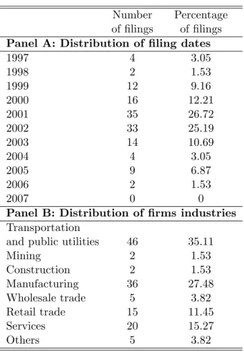
Table 2 provides information on the …ling dates as well as the industry distribution. Not surprisingly and as shown by Panel A, the majority of …rms in our sample …led for Chapter 11 during the 2001–2002 recession.
5
Montgomery Wald Holding …led for Chapter 11 in 07/07/1997 and then in 12/28/2000. McLeod USA INC defaulted in 1/30/2002, emerged and then defaulted again in 2005. U.S. Airways was reported as Pas-senger Airline that entered into Chap 11 in 08/11/2002 and then as Holding company for PasPas-sengers Airlines that defaulted in 09/12/2004. For each of these companies, we keep both default events as observations in our sample.
5.2 Model calibration
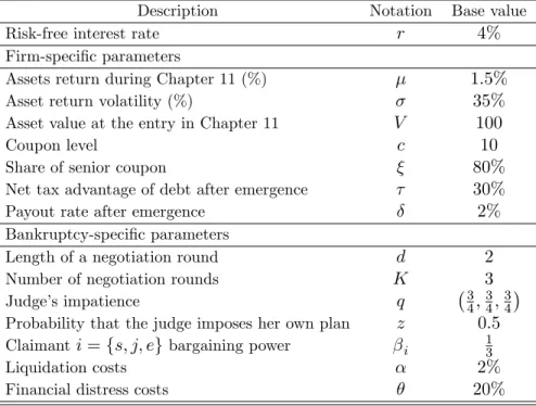
The average 10–year Constant Maturity Treasury (CMT) over the 1997-2007 period is 3.83%. Consequently, we set r = 4%. Apart from the risk-free rate, the parameters of our model can be classi…ed into two categories: …rm-speci…c parameters and bankruptcy-speci…c parameters. Table 3 summarizes the calibration results.
5.2.1 Firm-speci…c parameters
These parameters must characterize a typical …rm initiating a Chapter 11 …ling. We …rst compute the series of quarterly log-returns on assets for the 131 sample …rms over the two years prior to their entry in Chapter 11. Median values for the expected return and volatility of assets returns are 1.41% and 34%, respectively. Accordingly, we set = 1:5%
and = 35%.
For each …ling …rm, the coupon rate (in percentage of asset value) is obtained by multi-plying book leverage with the risk-free rate. Book leverage is calculated from the quarterly balance sheet on the eight quarters preceding Chapter 11 …ling, that is, for …rm n
Book leveragen= 1 8
8 X i=1
Total debtn;i
Total debtn;i+ Total equityn;i ,
where total equity is approximated by
Total equityn;i = Common equityn;i Purchase of common and preferred stocksn;i+ Sale of common and preferred stocksn;i,
and total debt is approximated by
Total debtn;i= Long term debtn;i+ Debt in current liabilitiesn;i.
Our coupon rate (c = 10 with V = 100) is the rounded value of the median coupon rate (0.1077).
The share of senior debt is computed from the annual balance sheet over the two years preceding Chapter 11 …ling as6
n= 1 1 2 2 X i=1
Debt subordinatedn;i Long term debtn;i . The median of all n is 81.13%, so we set = 80%.
For …rms emerging from Chapter 11, we set the net tax advantage of debt equal to 30%, in line with the estimates of Graham and Mills (2008), and the payout rate equal to 2%, in line with the estimates of Ericsson and Reneby (2005).
5.2.2 Bankruptcy-speci…c parameters
In our model, the bankruptcy procedure is completely characterized by the maximum num-ber of negotiation rounds, the duration of each bargaining round, the probabilities of the judge’s interference and cramdown, and the vector re‡ecting the judge’s own reorganiza-tion plan. We also need to specify the costs associated to the procedure.
Carapeto (2005) shows that on a sample of 144 Chapter 11 …rms that reorganized successfully and had more than one plan over the period 1986–1997, the average number of reorganization plans is 3.2. Moreover, she shows that about two-thirds of Chapter 11 …rms require more than one plan before an agreement can be attained. Consequently, we assume a total number of negotiation rounds K = 3, thus allowing each claimant to present their reorganization plan. Furthermore, the recently amended paragraph 1121 of the Bankruptcy Code states that the 180-day period for obtaining plan approval may not be extended beyond 20 months. We therefore set bargaining rounds of constant length d = 2 years. These parameters lead to a maximum procedure of 6 years, which is roughly consistent with empirical studies on Chapter 11 durations. For instance, Bris, Welsch and Zhu (2006), Denis and Rodgers (2007), and Kalay, Singhal and Tashjian (2007) document durations of Chapter 11 ranging from less than one year to more than 8 years.
As far as the judge behavior is concerned, we assume that her impatience is constant
during the reorganization process,7 and we assume there is 75% chance (i.e. qk = 34 for 1 k K) that she intervenes.8 We further assume the judge is equally likely to impose the last proposed plan or her own. Accordingly, we set z = 0:5. Finally, to reinforce the fairness and equity characteristics of the judge’s plan, it is reasonable to assume that the residual value is equally distributed among the claimants, leading to a sharing vector
= 13;13;13 .
In our model, bankruptcy costs are broken down into two components: liquidation and …nancial distress costs. Liquidation costs are proportional to the current asset value by a factor : Financial distress costs are assumed proportional to the length of the process and are characterized by a factor .
The empirical literature o¤ers di¤erent estimation methods and a wide range of values for bankruptcy costs. We use the estimates provided by Bris et al. (2006) as inputs to our model. Our choice is motivated by the following reasons. First, these estimates are based on the largest Chapter 11 sample in the literature.9 Second, their sample provides estimates of both the liquidation and …nancial distress costs. Third, their sample period, which ranges from 1995 to 2001, is close to ours. In addition, they estimate direct …nancial distress costs as a proportion of the assets value at the entry at Chapter 11. Therefore, we use liquidation costs of 2%. Bris et al. (2006) …nd average direct …nancial distress costs equal to 9.5%. Not
7
The assumption of constant interference probability results from two opposite considerations. On one hand, Baird and Morrison (2001) point out that the judge holds the option to determine the renegotiation outcome and, as predicted by real options theory, is better o¤ waiting for the arrival of new information (i.e. the judge becomes more patient with time). On the other hand, welfare concerns induce the judge to accelerate the costly procedure (i.e. the judge becomes less patient with time).
8
Although we could not …nd direct evidence on judge intervention frequency, Evans (2003) documents frequent judicial discretionary actions in Chapter 11. For instance, among the 290 cases in her sample, the judge decided to alter the exclusivity period (i.e. the length of the …rst round) in 120 cases. She also …nds signi…cant di¤erences in discretionary actions as well as bankruptcy outcomes across judges – reinforcing the idea that judge behaviour is not entirely predictable by claimholders.
9Altman (1984) uses a sample of 19 cases, Weiss (1990) uses 37 cases, Betker (1997) 75 cases, Lubben
(2000) 22 cases, and LoPucki and Doherty (2004) 48 cases, while Bris et al. (2006) use a sample of 300 large …lings.
much is reported about indirect …nancial distress costs, but if we assume comparable order of magnitude, the total (direct and indirect) …nancial distress costs amount to 20% of the assets value at the entry in Chapter 11 per year.
6
Analysis of results
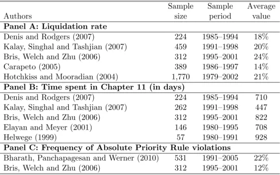
We start by reporting the main output of the model, namely the di¤erent plans proposed at each round as a function of asset value. This allows us to identify the possible equilibria and their corresponding range for asset value. Next, we infer the probabilities associated to each outcome, the average time spent in Chapter 11 as well as the frequency of violations from the Absolute Priority Rule (APR) – three quantities that we can relate to empirical data.
6.1 Proposed plans
Figure 1 depicts the plans proposed by the di¤erent classes of claimholders during the three rounds. These plans are summarized by the triplet of …rm value fractions that are o¤ered to each class of claimants.
For each round, there is a critical threshold for asset value below which the …rm is liquidated. This threshold corresponds to the accumulated coupon payments and costs of …nancial distress, and therefore increases with the next round. Above this threshold, a reorganization plan is actually proposed.
Figure 1a shows the plans proposed by shareholders during the …rst round. For a su¢ ciently high level of asset value (around 62 in our base case), shareholders have no interest in making concessions with creditors, as they expect the …rm to be wealthy enough to obtain better terms in the future. That is why they voluntarily o¤er a plan leaving nothing to senior creditors and a minimal share to junior creditors (to obtain their vote and avoid liquidation). Shareholders expect this plan to be either rejected –which will lead negotiations to the next round – or to be crammed down by the judge, giving them either “the fair and equitable” share or an extremely favorable outcome to them.
As asset value goes lower, the likelihood of liquidation increases and induces shareholders to make concessions. As a matter of fact, they o¤er a plan that is accepted by both creditors when asset value lies within 48 and 62.
But if asset value gets very close to the liquidation threshold (between 40 and 48 in our base case), shareholders’ value becomes so small that they have an incentive to o¤er the plan that, again, shares nothing with senior creditors, and gives the smallest possible share to junior creditors. This “desperate” plan is motivated by the fact that, in expectation, shareholders are better o¤ gambling on the judge intervention as they have almost nothing left to lose.
A similar logic applies to the second round. Figure 1b shows that, when asset value is high enough, senior creditors will grant themselves almost all of …rm value, leaving just a small fraction to shareholders to get their vote. Shareholders’ acceptance is cheaper to buy since they are last in priority. Again, worst case for senior creditors is that the plan is rejected and negotiations move on to the third round. At best, the judge may cram down this plan that is extremely favorable to them.
For a wide set of intermediate values of asset (between 100 and 300 in our base case), senior creditors are better o¤ reaching the unanimous consent, and the proposed shares re‡ect the relative priority of the three claimants.
As asset value gets very close to the liquidation threshold, senior creditors behave in a similar fashion as shareholders in the …rst round, as they o¤er again a “desperate” plan granting a minimal fraction to shareholders.
The logic is simpli…ed when it comes to the third round since it is the last round. Junior creditors, who are now the leader, know they cannot expect negotiations to continue. But since they are last in priority, they …nd no bene…t in making concessions. Hence the only plan they propose is the minimal fraction that warrants shareholders acceptance and the rest of …rm value to them (see Figure 1c). Clearly, this plan can only be adopted but with judge cramdown.
6.2 Equilibrium probabilities
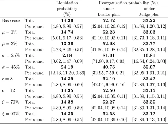
We compute, for each round k, the probability that the geometric Brownian motion, initially starting at v = V0 at the entry in Chapter 11, ends up in the domain of each equilibrium. These probabilities then need to be adjusted for judge intervention: In case of partial acceptance of the plan, there is a probability qk that the judge imposes a plan (her own with probability z and the last proposed plan with probability 1 z). This allows us to …nally determine, for each round, the probabilities of liquidation, reorganization under the leader’s plan and reorganization under the judge’s plan (see Appendix C for details). Results are summarized in Tables 4 and 5.
Our calibrated base case yields a liquidation probability (14.36%) that is in line with observed liquidation rates in Chapter 11 procedure. Table 6 Panel A surveys the liquidation rates reported by most recent empirical studies on Chapter 11 …lings from public …rms. These rates lie between 14% and 24%, indicating a strong consensus between observed liquidation likelihood and our base case parameterization. Interestingly, the conditional liquidation probability of our model increases as one moves from one round to another, indicating the decay in reorganization possibilities as time passes.
There is approximately one third of chances that the judge will cramdown the "fair and equitable" plan, mostly after the …rst round. Unfortunately, we cannot relate this …gure to any statistics about judge intervention. Our base case otherwise indicates that the most likely outcome is reorganization under shareholders’plan (42.04% of probability). The probability of getting to the third round is small but this is caused by our stylized assumptions of three rounds of equal duration. As we will see in the next subsection, our calibration yields an overall Chapter 11 duration that is consistent with observations.
Equilibrium probabilities display great sensitivity to asset volatility. Consistent with intuition, very risky …rms become more likely to be liquidated (probability increases to 24%), while safer …rms have greater chances of being reorganized under the Leader’s plan – mostly shareholders’ plan after the …rst round. Other sensitivities with …rms-speci…c parameters are much smaller and in line with expectations (see Table 4). The …rm will
avoid liquidation and enjoy a reorganization plan as asset drift is higher and leverage is higher. This is in line with Denis and Rodgers (2007) who …nd a positive relation between the reorganization likelihood and the change in operating margin on one hand (although not signi…cant), and the liability ratio prior to …ling Chapter 11 on the other hand. We further note from Table 4 that liquidation probability slightly decreases as the junior creditor is less important. This is mostly explained by the fact that senior creditors will …nd it easier to have their plan accepted after the second round.
As far as bankruptcy-speci…c parameters are concerned, we note that when the judge can credibly signal her intention to impose her own plan (i.e. higher z), then claimholders have a stronger incentive to reach an agreement by themselves. As shown in Table 5, probability of liquidation as well as that of reorganization under the judge plan sharply decrease. The bene…ts of this incentive accrue to shareholders as they …rst propose a plan (compared to base case, the probability of reorganization under their plan goes from 52.42% to 70.50% as z goes from 0.5 to 0.65). As expected, liquidation probability decreases with costs of liquidation, but this e¤ect is economically small. By contrast, costs of …nancial distress turn out to be a more important driver of outcome probabilities. A very costly procedure (say = 30%) reduces the scope for renegotiation and makes early liquidation more likely. The same e¤ect is obtained by increasing the length of a round. As d goes from 2 years (base case) to 3 years, liquidation probability increases (mostly in the …rst round) at the expense of all reorganization probabilities.
6.3 Chapter 11 duration
By weighting the length of each round with the corresponding probability of reorganiza-tion (either under Leader or judge plan), we can compute the model-implied durareorganiza-tion of reorganization under Chapter 11. With the base case, we obtain an average duration of
365 2 42:04 + 31:89 52:42 + 33:22+ 4 10:26 + 1:2 52:42 + 33:22+ 6 0:12 + 0:12 52:42 + 33:22 ;
studies. This length of time lies within 708 and 915 days, with the exception of the study by Kalay et al. (2007) who …nd a signi…cantly shorter Chapter 11 duration (447 days on average).
As expected, higher costs of …nancial distress induce claimholders to spend less time in renegotiations (average time to reorganization decreases to 794 days when = 30%). A similar remark holds when the judge is more prone to imposing her own plan (average time to reorganization decreases to 796 days when z = 0:65). Other sensitivities are not economically meaningful, so we do not report them.
6.4 APR violations
From our model simulations, it is straightforward to infer the probability that the Absolute Priority will not be respected. Indeed, each claimholder votes in favor of the proposed plan provided the fraction of …rm value they get is at least equal to the one obtained from the Absolute Priority Rule. As a consequence, deviations from the APR only occur when the following three conditions are met: (i) the plan is rejected, (ii) the judge intervenes, and (iii) she imposes the Leader’s plan (and not the fair and equitable one).
The probability of deviation from the APR is therefore equal to the probability of reorganization under judge plan (as reported in Tables 4 and 5) multiplied by 1 z. Thus, our base case parameters yield a probability of APR violations of 16.61%. This …gure is consistent with recent empirical estimates as reported from Table 6, Panel C.
7
Conclusion
In this paper, we have developed and solved a non-cooperative game approach to model renegotiations under the bankruptcy law. By doing so, we hope to contribute to the mod-elling of …nancial distress in the contingent claims literature, by opening "the black box" of Chapter 11 bargaining process. We show that rational claimholders can assess the likeli-hood of bankruptcy outcomes (liquidation or reorganization under di¤erent types of plans), using information about the …rm and the legal procedure. Our approach uses a simple
information structure and only relies on the perceived randomness of the judge’s actions – which is su¢ cient to generate multiple-round bargaining and multiple equilibria. A proper calibration of the model yields liquidation rate, Chapter 11 duration and percentage of devi-ations from the Absolute Priority Rule that are in line with statistics reported by empirical studies. The model also generates predictions as to how these observables are a¤ected by changes in …rm-speci…c or bankruptcy-speci…c parameters.
Admittedly, the modelling of negotiations under Chapter 11 could incorporate additional aspects that would possibly enrich the analysis, but also make the approach less tractable. For instance, informational asymmetries (i.e. shareholders and management having a more accurate knowledge of asset dynamics than creditors) could alter the equilibria of the game. In addition, con‡icting interests between management and shareholders could modify the type of proposed plan – managers being primarily concerned with avoiding liquidation to keep their job. Li and Li (1999) argue however, that informational asymmetries and agency problems are less severe in legal bankruptcy than in private renegotiations, as claimholders are forced to disclose information.
Another direction for future research is to model more explicitly the role of the judge. Among the judge’s primary goals, the literature on bankruptcy design (see e.g. Aghion, Hart and Moore, 1992) commonly cites: preserving the bonding role of debt (by enforcing the Absolute Priority Rule) and ensuring the bankruptcy procedure acts as an e¢ cient "…lter" for distressed …rms (i.e. liquidating insolvent …rms while reorganizing pro…table ones). More personal career concerns (such as in‡uence or prestige) could also be incorporated. This type of research direction is not trivial, as the judge ’s objective function is, in essence, multi-dimensional.
References
[1] Aghion, P., Hart, O., and Moore, J., 1992. The Economics of Bankruptcy Reform. Journal of Law, Economics and Organization 8, 523–546.
[2] Altman, E. I., 1984. A Further Empirical Investigation of the Bankruptcy Cost Ques-tion. Journal of Finance 39, 1067–1089.
[3] Anderson, R., and Sundaresan, S., 1996. The Design and Valuation of Debt Contracts. Review of Financial Studies 9, 37–68.
[4] Baird, D., and Morrison, E., 2001. Bankruptcy Decision Making. Journal of Law, Economics and Organization 17, 356–372.
[5] Berkovitch, E., Israel, R., and Zender, J., 1998. The Design of Bankruptcy Law: A Case for Management Bias in Bankruptcy Procedures. Journal of Financial and Quantitative Analysis 33, 441–64.
[6] Betker, B. L., 1997. The Administrative Costs of Debt Restructuring: Some Recent Evidence. Financial Management 26, 56–68.
[7] Bharath, S., Panchapegesan, V., and Werner, I., 2010. The Changing Nature of Chapter 11. Working Paper, University of Michigan.
[8] Bris, A., Welch, I., and Zhu, N., 2006. The Costs of Bankruptcy: Chapter 7 Liquidation versus Chapter 11 Reorganization. Journal of Finance 61,1253–1303.
[9] Broadie, M., Chernov, M., and Sundaresan, S., 2007. Optimal Debt and Equity Values in the Presence of Chapter 7 and Chapter 11. Journal of Finance 62, 1341–1377. [10] Brown, D., 1989. Claimholder Incentive Con‡icts in Reorganization: The Role of
Bank-ruptcy Law. Review of Financial Studies 2, 109–123.
[11] Bruche, M., and Naqvi, H., 2010. A Structural Model of Debt Pricing with Creditor-Determined Liquidation. Journal of Economic Dynamics & Control 34, 951–967. [12] Carapeto, M., 2005. Bankruptcy Bargaining with Outside Options and Strategic Delay.
[13] Chang, T., and Schoar, A., 2008. Judge Speci…c Di¤erences in Chapter 11 and Firm Outcomes. Working Paper. MIT and NBER.
[14] Datta, S., and Iskandar-Datta, M. E., 1995. Reorganization and Financial Distress: An Empirical Investigation. Journal of Financial Research 18, 15–32.
[15] Davydenko, S. A., 2010. When Do Firms Default? A Study of the Default Boundary. Working Paper. University of Toronto.
[16] Denis, D. K., and Rodgers, K. J., 2007. Chapter 11: Duration, Outcome, and Post-Reorganization Performance. Journal of Financial and Quantitative Analysis 42, 101– 118.
[17] Eberhart, A. C., Moore, W. T., and Roenfeldt, R. L., 1990. Security Pricing and Deviations from the Absolute Priority Rule in Bankruptcy Proceedings. Journal of Finance 45, 1457–1469.
[18] Elayan, F., and Meyer, T., 2001. The Impact of Receiving Debtor-in-Possession Fi-nancing on the Probability of Successful Emergence and Time Spent Under Chapter 11 Bankruptcy. Journal of Business Finance and Accounting 28, 905–942.
[19] Ericsson, J., and Reneby, J., 2005. Estimating Structural Bond Pricing Models. Journal of Business 78, 707–735.
[20] Evans, J., 2003. The E¤ect of Discretionary Actions on Small Firms’Ability to Survive Chapter 11 Bankruptcy. Journal of Corporate Finance 9, 115–128.
[21] Fan, H., and Sundaresan, S., 2000. Debt Valuation, Renegotiation, and Optimal Divi-dend Policy. Review of Financial Studies 13, 1057–1099.
[22] François, P., and Morellec, E., 2004. Capital Structure and Asset Prices: Some E¤ects of Bankruptcy Procedures. Journal of Business 77, 387–411.
[24] Gertner, R., and Scharfstein, D., 1991. A Theory of Workouts and the E¤ects of Re-organization Law. Journal of Finance 46, 1189–1222.
[25] Giammarino, R. M., 1989. The Resolution of Financial Distress. Review of Financial Studies 2, 25–47.
[26] Gilson, S., John, K., and Lang, L., 1990. Troubled Debt Restructurings: An Empirical Study of Private Reorganization of Firms in Default. Journal of Financial Economics 27, 315–353.
[27] Graham, J., and Mills, L., 2008. Using Tax Return Data to Simulate Corporate Mar-ginal Tax Rates. Journal of Accounting and Economics 46, 366–388.
[28] Hackbart, D., Hennessy, C., and Leland, H., 2007. Can the Tradeo¤ Theory Explain Debt Structure? Review of Financial Studies 20, 1389–428.
[29] Hege, U., and Mella-Barral, P., 2005. Repeated Dilution of Di¤usely Held Debt. Journal of Business 78, 737–86.
[30] Helwege, J., 1999. How Long Do Junk Bonds Spend in Default? Journal of Finance 54, 341–357.
[31] Hotchkiss, E., and Mooradian, R., 2004. Post-Bankruptcy Performance: Evidence from 25 Years of Chapter 11. Working Paper. Boston College and Northeastern University. [32] Kalay, A., Singhal, R., and Tashjian, E., 2007. Is Chapter 11 Costly? Journal of
Financial Economics 84, 772–796.
[33] Li, D., and Li, S., 1999. An Agency Theory of the Bankruptcy Law. International Review of Economics & Finance 8, 1–24.
[34] Leland, H., 1994. Corporate Debt Value, Bond Covenants, and Optimal Capital Struc-ture. Journal of Finance 49, 1213–1252.
[35] LoPucki S. J., and Doherty, J. W., 2004. The Determinants of Professional Fees in Large Bankruptcy Reorganization Cases. Journal of Empirical Legal Studies 1, 111– 141.
[36] Lubben, S. J., 2000. The Direct Costs of Corporate Reorganization: An Empirical Examination of Professional Fees in Large Chapter 11 Cases. American Bankruptcy Law Journal 509, 508–552.
[37] Luther, K., 1998. An Arti…cial Neural Network Approach to Predicting the Outcome of Chapter 11 Bankruptcy. Journal of Business and Economic Studies 4, 57–73. [38] Mella-Barral, P., 1999. The Dynamics of Default and Debt Reorganization. Review of
Financial Studies 12, 535–578.
[39] Mella-Barral, P., and Perraudin, W., 1997. Strategic Debt Service. Journal of Finance 52, 531–556.
[40] Merton, R., 1974. On the Pricing of Corporate Debt: The Risk Structure of Interest Rates. Journal of Finance 29, 449–470.
[41] Moraux, F., 2002. Valuing Corporate Liabilities when the Default Threshold is not an Absorbing Barrier. Working Paper. University of Rennes I.
[42] Weiss, L., 1990. Bankruptcy Resolution: Direct Costs and Violation of Priority of Claims. Journal of Financial Economics 27, 285–314.
[43] Weiss, L., and Wruck, K. H., 1998. Information Problems, Con‡icts of Interest, and Asset Stripping: Ch.11’s Failure in the Case of Eastern Airlines. Journal of Financial Economics 48, 55–9.
[44] White, M., 1996. The Costs of Corporate Bankruptcy: A U.S.-European Comparison. In Bhandari J., Economic and Legal Perspectives, Cambridge UK: Cambridge Univer-sity Press.
Appendix
Appendix A: Reorganization plans
We …rst show that the judge’s vector of weights ; along with sharing rule (15), de…nes a unique reorganization plan c at (v; k). We then derive the analytic solution to the optimization problem (18)-(19) for all combinations of decisions by the followers, and all possible identities of the leader.
Using the auxiliary variable y de…ned in (20) in (8) and (10), the reorganization value of the …rm, the equityholders, and of the creditors can be written as follows for y 2 [0; 1] :
!RF(v; y; k) = wk + y 1 1 + y 1 1 (23) !Re(v; y; k) = wk y + (1 ) y11 (24) !Rd (v; y; k) !Rs (v; y; k) + !Rj (v; y; k) (25) = wk 1 1 y 1 1 (1 ) y 1 1 :
Bankruptcy judge’s plan
For a given asset value v at negotiation round k, the reorganized coupon pair c (v; k) satisfying (15) is obtained by solving
!Re(v; c ; k) e !RF(v; c ; k) (1 ) wk = !Le(v; k). (26) Replacing !RF and !Re by their expression in (23)-(24) and rearranging yields
y 1 + e 1 y 1 1 1 + e +1 = 1 e ! L e(v; k) wk
Di¤erentiating the l.h.s. with respect to y, we obtain that the …rst derivative vanishes
when y1 = (1 (1 e))(1 )
(1 )(1 )+ e( + (1 )) 2 (0; 1) : Moreover, the second derivative is
y21 1(1 ) (1 ) + e( + (1 ))
(1 )2(1 ) < 0:
We obtain that the l.h.s. is concave in y and admits a maximum in (0; 1). Moreover its value is 0 at y = 0, while it is (1 e) > 0 at y = 1. Therefore, there is a unique solution to (26) corresponding to a value for y in [0; 1] since 0 !Le(v;k)
wk (1 ), yielding 0 1 e ! L e(v; k) wk (1 e) :
Leader’s optimal plan
D = (A; A) If both followers accept the plan, then the outcome vector is !R(v; c; k). In that case, the leader’s best proposal is the solution of
max c ! R 0(v; c; k) (27) s.t. !Ri (v; c; k) qk z!Ri v; c ; k + (1 z)!Ri (v; c; k) + (1 qk)!Ci (v; k); (28) or, equivalently, !Ri (v; c; k) bi; (29) bi = 8 < : qkz!Ri(v;c ;k)+(1 qk)!Ci(v;k) 1 qk(1 z) if qk(1 z) < 1 1 otherwise. ; i 2 f1; 2g : (30)
where condition (28) is obtained by comparing the reorganization payo¤ with the expected outcome when one of the followers accept the plan, while the other rejects it (see Table 1).
D = (A; R) or (R; A) If Follower 1 accepts the plan while Follower 2 rejects it, then the outcome vector is
The leader’s best proposal in that case is the solution of max c ! R 0(v; c; k) (31) s.t. qk z!R1 v; c ; k + (1 z)!R1 (v; c; k) + (1 qk)!C1(v; k) qk!L1(v; k) + (1 qk)!C1(v; k) (32) and qk z!R2 v; c ; k + (1 z)!R2 (v; c; k) + (1 qk)!C2(v; k) !R2(v; c; k); or equivalently !R1 (v; c; k) b1; b1 = 8 < : !L 1(v;k) z!R1(v;c ;k) 1 z if z < 1 and qk> 0 1 otherwise, (33) and !R2 (v; c; k) b2; b2 = 8 < : qkz!R2(v;c ;k)+(1 qk)!C2(v;k) 1 qk(1 z) if qk(1 z) < 1 qk!R2 v; c ; k + (1 qk)!C2(v; k) otherwise. (34)
where the constraints are obtained by comparing what Follower 1 may expect if he rejects the plan and what Follower 2 may expect if he accepts the plan. The leader’s best proposal corresponding to the decision pair (R; A) is obtained by changing the identity of the followers.
D = (R; R) If both followers reject the plan, the outcome vector is qk!L(v; k) + (1 qk) !C(v; k)
which does not depend on the coupon proposed by the leader, as long as it leads the followers to reject the plan. It su¢ ces that the leader propose nothing to both followers to achieve this outcome.
The optimization problems (27)-(28) and (31)-(32) involve the reorganization values !Ri : Using the auxiliary variable y de…ned in (20) and di¤erentiating (24) with respect to y yields
wk
1 y1 < 0 if y 2 [0; 1] ;
which shows that the reorganization value of the equityholder is decreasing in y on [0; 1], with !Re(v; 0; k) = wkand !Re(v; 1; k) = 0: Similarly, it is straightforward to verify that the total creditors’reorganization value !Rd (v; y; k) is concave in y and admits a maximum at
y = 1
1 (1 ) (1 )
(1 )=
2 [0; 1] , (35)
with !Rd (v; 0; k) = 0 and !Rd (v; 1; k) = wk(1 ) : These properties of the reorganization values allow to characterize the leader’s optimal plan analytically at any (v; k) :
Equityholder’s plan
D = (A; A) When the leader is the equityholder, the solution of problem (27)-(28) is ob-tained by o¤ering the lower bound on their payo¤ to both followers, as de…ned by (29). The optimal reorganization plan for the equityholder is therefore obtained by solving for y the following:
!Rd (v; y; k) = bs+ bj; (36)
where !R
d (v; y; k) 2 [0; wk(1 )].
i If 0 < bs+ bj < wk(1 ) , then there is a unique y 2 (0; 1) corresponding to a unique total coupon satisfying (36), which is the solution to problem (27)-(28). ii If wk(1 ) < bs+ bj while !Rd (v; y ; k) is positive, then there are two values
iii If wk(1 ) < bs+ bj while !Rd (v; y ; k) is negative, then the equityholder is not able to o¤er their lower bounds to the creditors, and it is not possible for him to propose a plan that will be accepted by both creditors.
iv If bs+ bj 0 while wk(1 ) > bs+ bj, then the solution to problem (27)-(28) is y = c = 0.
The relative share of the total coupon which is o¤ered to the senior and junior creditors can then easily be determined by solving (9) for the senior debt coupon cs, given y. D = (A; R) or (R; A) The solution of problem (31)-(32) is obtained by o¤ering the lower
bound b1 in (33) to Follower 1, and nothing to Follower 2. First, select the identity of Follower 1 by choosing
arg min i2fs;jg
n
!Li(v; k) z!Ri v; c ; k o. (37)
The optimal reorganization plan for the equityholder is then obtained by solving for y the following:
!Rd (v; y; k) = b1, (38)
using (13). If 0 < b1 < wk(1 ) , then there is a unique y 2 [0; 1] corresponding to a unique coupon satisfying (38), which is the solution to problem (31)-(32); the other possible cases are obtained similarly as for problem (27)-(28) above.
Creditor’s plan
If the leader is one of the creditors, he maximizes his share in the reorganized …rm by deciding both on the total coupon and on the relative share of the other creditor, which we will label f . For a given total coupon, the leader’s objective function is decreasing in the share of the other creditor, so that it is optimal to o¤er Creditor f the lower bound on his payo¤. Therefore, the objective functions (27) and (31) can both be written:
!Rd (v; y; k) bf (39)
D = (A; A) In problem (27)-(28), the followers’payo¤s bf and be are de…ned by (29). i If !Rd (v; y ; k) < bf, then it is not possible for the leader to o¤er a plan that will be
accepted by both followers.
Otherwise, if !Rd (v; y ; k) bf, then we check if plan y satis…es the equityholders or not.
ii If !Re (v; y ; k) be, then the optimal plan corresponds to y . The relative share of the two creditors in the reorganized coupon is obtained by solving !R
f (v; y ; k) = bf. iii If !R
e (v; y ; k) < be, the leader has to o¤er be to the equityholders, by proposing a plan that solves
wk
y + (1 ) y11 = be: (40)
Since the equity value is decreasing in y, then if wk be, there is a unique solution in [0; 1] to (40), denoted yb. If !Rd v; yb; k bf, the optimal plan for the leader is yb and the relative share of the two creditors in the reorganized coupon is obtained by solving
!Rf v; yb; k = bf: (41)
iv If wk< be or !Rd v; yb; k < bf; then it is not possible for the leader to o¤er a plan that will be accepted by both followers.
D = (A; R) or (R; A) The solution of problem (31)-(32) depends on the identity of Fol-lower 1, who accepts the plan. The leader chooses the identity of FolFol-lower 1 by comparing his share in the two following cases.
i If Follower 1 is the equityholder, then the leader maximizes his share by o¤ering nothing to the other creditor, cf = 0. If !Re (v; y ; k) be, then the optimal plan corresponds to y , whereas if !Re (v; y ; k) < beand wk be; then the optimal plan corresponds to yb. If wk< be, it is not possible for the leader to o¤er a plan that will be accepted by
ii If Follower 1 is the other creditor, then if !Rd (v; y ; k) < bf, it is not possible for the leader to o¤er a plan that will be accepted by Follower 1. Otherwise, the leader maximizes his share by proposing plan y , and the relative share of the two creditors is obtained by solving (41).
Appendix B: Numerical implementation
The value of what each claimant expects to recover from the Chapter 11 negotiation proce-dure at a given date t = kd; k = 0; :::; K is a function of the value of the …rm’s assets at that date obtained by solving the stochastic dynamic program (??)-(??) by backward induction from the last negotiation round, using (21), (16) and (17). Since the state space of the dynamic program is continuous, the …rst step is to partition it into a collection of convex subsets, and obtain a corresponding …nite set of grid points where the value functions are to be evaluated. Piecewise-linear continuous interpolation functions are then de…ned to approximate the value functions over the state space.
Let g0 < g1 < ::: < gm < ::: < gM de…ne a grid G on the space of asset values, and let g0 = 0 and gM +1 = +1. Assume that approximations of the value functions, denoted by ~!i, i 2 fs; j; eg; are known on G. We de…ne continuous piecewise linear interpolation functions ^!i on R such that at t = kd, ^!i(v; k) = ~!i(v; k) on G and
^ !i(v; k) = 8 < : 0 for v < g0 akim+ hkimv for gm v gm+1, m = 0; :::; M = M X m=0 akim+ hkimv 1 (gm v < gm+1) (42)
where 1 ( ) is the indicator function.
The coe¢ cients akimand hkimof the piecewise linear interpolation functions are obtained by setting ^!i(v; k) = ~!i(v; k) on the grid and by extrapolating outside the grid. They are
given by aki0 = 0 hki0 = !~i(g1; k) g1 akim = gm+1!~i(gm; k) gm!~i(gm+1; k) gm+1 gm ; m = 1; :::; M 1 hkim = !~i(gm+1; k) !~i(gm; k) gm+1 gm ; m = 1; :::; M 1 akiM = akiM 1 hkiM = hkiM 1: (43)
Using the interpolated value functions in (42) at v = gn; n = 1; : : : M; yields for k = 0; :::; K 1 and t = kd e rdEvt[^!i(Vt+d; k + 1)] = e rdEvt " M X m=0 ak+1im + hk+1im Vt+d Im # = M X m=0 Anm!~i(gm; k + 1) (44)
where Im denotes the indicator function of the event fgm Vt+d< gm+1g. Using (43), the transition parameters Anm; from state v = gnat t to the interval [gm; gm+1) at t + d; which are constant under our assumption of equal length negotiation rounds, are then given by
Anm= 8 > > > > < > > > > : e rdEvt hg 1 Vt+d g1 g0 I0 i for m = 0 e rdEvt hV t+d gm 1 gm gm 1 Im 1+ gm+1 Vt+d gm+1 gm Im i for 1 m < M e rdEvt hV t+d gm 1 gm gm 1 (Im 1+ Im) i for m = M: (45)
Recall that, according to our assumption (1) about the assets value process, at v = gn Evt(Im) = (xn;m+1) (xnm) Evt(Vt+dIm) = gn xn;m+1 p d xnm p d (46)