CIRPÉE
Centre interuniversitaire sur le risque, les politiques économiques et l’emploi
Cahier de recherche/Working Paper 06-14
The Returns to Computer Use Revisited, Again
Benoit Dostie
Rajshri Jayaraman
Mathieu Trépanier
Avril/April 2006
_______________________
Dostie: Corresponding author. Institute of Applied Economics, HEC Montréal, University of Montréal, Montréal (Québec), H3T 2A7; IZA, CIRANO, CIRPÉE and CREF
Jayaraman: Center for Economic Studies, CESifo and University of Munich
Trépanier: Kellogg School of Management, Northwestern University, Evanston (Illinois)
We thank Larry Blume, Richard Chaykovsky, Rob Clark, Nicole Fortin, Avi Goldfard, David Green, Paul Lanoie, Pierre Thomas Léger, Thomas Lemieux, Asaf Razin, Paul Ruud, Klaus Schmidt, Michael Smart, Pierre-Yves Steunou and participants in the 2004 CEA and SCSE Conferences for valuable comments. We greatfully acknowledge financial support from the Social Sciences and Humanities Research Council of Canada through the Initiatives on the New Economy program, Human Resources and Skills Development Canada and HEC Montréal. The usual caveat applies.
Abstract: Using North American data, we revisit the question first broached by
Krueger (1993) and re-examined by DiNardo and Pischke (1997) of whether there
exists a real wage differential associated with computer use. Employing a mixed
effects model to correct for both worker and workplace unobserved heterogeneity
using matched employer-employee panel data, we find that computer users enjoy an
almost 4 per cent wage premium over non-users. Failure to correct for the worker
selection effect leads to a more than twofold overestimate of this premium, as does
failure to correct for workplace unobserved heterogeneity.
Keywords: Wage determination, Computers, Mixed models, Linked
employer-employee data
1
Introduction
The question of whether or not there exists a premium to computer use was famously addressed by Krueger (1993) who concluded, using cross-sectional data from the U.S., that computer users earned a 15 to 20 per cent wage premium over nonusers. This …gure was widely quoted until DiNardo and Pischke (1997) cast a shadow of doubt over Krueger’s methodology. Using cross-sectional data from Germany, DiNardo and Pischke (1997) observed that computer users enjoyed a similar wage premium, but so did workers who used pencils or pens and those who sat down while working. Since such tools as writing implements and chairs are, in and of themselves, unlikely to yield large increases in productivity, they interpreted their …ndings as suggestive evidence that the observed computer premium may simply be a return to unobserved skills.
In North America, the debate regarding whether or not computer users enjoy a wage premium has pretty much languished there.1 This is unfortunate: given
that computers arguably constitute the single most pervasive manifestation of skill-biased technological change, and skill-biased technological change is widely thought to be responsible for widening wage disparities observed in the U.S. and Canada since the 1970s, it is important to understand whether or not there exists a direct link between computers and wages.2
There is widespread consensus regarding what the data do not conclusively say, but there has been virtually no exploration of what they do actually say. Indeed, there appears to be something of a consensus based on Dinardo and
1Several recent papers have examined the e¤ect of technological change on individual wages
using European data. Dolton and Makepeace (2004) …nd a computer wage premium of 10-13% in Britain, while Anger and Schwarze (2003) in Germany, and Entorf and Kramarz (1997) and Entorf, Gollac, and Kramarz (1999) in France …nd no signi…cant premium. Of these only the last 2 utilise a matched employer-employe dataset, allowing one to correct for worker and workplace unobserved components and only the last paper corrects for these two simultaneously. We compare our results in Section 4.
2Acemoglu (2002) provides a comprehensive review of the literature on technological change
Pischke’s (1997) suggestive evidence that the returns to computer use are neg-ligible, if not zero.
Data limitations are probably the main culprit for the neglect of this is-sue. The most obvious way to explore whether the worker selection problem is responsible for observed wage di¤erentials or whether these wage di¤erentials are “real”, is by resorting to panel data containing information on both worker wages and computer use, and in North America such data are rare.
In this paper, we exploit a unique new (1999 2002) data set –the Canadian Workplace and Employee Survey (WES) –to examine the question of whether or not there exists a wage premium associated with computer use. WES is a lon-gitudinal, matched employer-employee data set, containing remarkably detailed information on workers and their workplaces.
The fact that we observe the same worker over time permits us to correct for the worker selection problem, thereby directly examining DiNardo and Pischke’s hunch for the …rst time in the North American context. In addition, the fact that the data are linked enables us to correct for workplace unobserved heterogeneity – a problem which was not the main focus of Dinardo and Pischke’s (1997) critique, but one with which Krueger (1993) grappled. We accomplish this by employing mixed e¤ects methods as suggested by Abowd and Kramarz (1999b).3
In the cross-section, using Krueger’s (1993) speci…cation, we …nd that com-puter use is associated with a 22 per cent wage premium. This number drops to just over 10 per cent once we correct for a rich array of observable character-istics, including experience with computer use. Once we correct for individual and workplace unobserved heterogeneity, the computer wage premium drops to
3To use standard …xed e¤ects, we would have to observe the same worker in di¤erent …rms
–a feature our data does not permit, therefore necessitating the use of this somewhat involved mixed model. We argue later, however, that …xed e¤ects methods may not be appropriate with short panels characterised by little variation. It is also worth noting that this mixed model does not require the orthogonality conditions pertaining to the unobserved components typically demanded of random e¤ects models. Moreover, it can be shown that …xed e¤ects estimates are a special case of mixed model estimates (see Abowd and Kramarz (1999b).)
3:8 per cent.
Our …ndings lend credence to DiNardo and Pischke (1997)’s suspicion: al-lowing for the possibility of worker selection roughly halves the computer wage premium. Interestingly, correcting for workplace e¤ects also leads to a sub-stantial reduction in the observed premium, suggesting that the large computer wage premium observed in the cross-section may re‡ect not only individual, but also workplace unobserved heterogeneity, perhaps mediated through managerial ability. Still, the fact that computer users in our data enjoy an almost 4 per cent wage premium relative to a non-user, even after our various corrections for unobservable as well as observable heterogeneity, as well as signi…cant returns to experience with computers suggests that there remains a sizeable return to computer use.
The remainder of the paper is organized as follows. Section 2 outlines our statistical framework, detailing our mixed model. Section 3 describes our data. In Section 4 we discuss our results, and Section 5 concludes.
2
Statistical Model
In order to take into account both individual and workplace heterogeneity in our model of wage determination, we use a two-factor analysis of covariance with repeated observations along the lines of Abowd and Kramarz (1999b):4
yit= + xit + i+ j(i;t)+ it, (1)
with
i= i+ ui , (2)
4Details about the model, estimation procedure as well as properties of the estimators
where yit is the (log) wage rate observed for individual i = 1; :::; N at time
t = 1; :::; Ti. Person e¤ects are denoted by i, workplace e¤ects by j as a
func-tion of i and t, and time e¤ects by t. is a constant, xitis a matrix containing
demographic information for worker i at time t as well as information concern-ing workplace j to which worker i is linked. Although and can be …xed or random, we assume they are …xed in our estimations. All other e¤ects are ran-dom. Personal heterogeneity ( i) is a measure of unobserved ( i) and observed
(ui ) time-invariant worker characteristics. Employer heterogeneity j
cap-tures workplace-speci…c unobserved characteristics, common to all workers of the same workplace. it is the statistical residual.
In full matrix notation, we have
y = X + U + D + F + (3)
where: y is the N 1 vector of earnings outcomes; X is the N q matrix of observable time-varying characteristics including the intercept; is a q 1 parameter vector; U is the N p matrix of time invariant person character-istics; is a p 1 parameter vector; D is the N N design matrix of the unobserved component for the person e¤ect; is the N 1 vector of person e¤ects; F is the N J design matrix of the workplace e¤ects; is the J 1 vector of pure workplace e¤ects; and is the N 1 vector of residuals.
In order to distinguish …rm from individual …xed e¤ects, we would have to observe the same worker in di¤erent …rms. Our sampling frame does not follow workers moving from …rm to …rm, therefore ruling out the option of treating both …rm and individual e¤ects as …xed.5 Instead, we employ a mixed
model in which worker and …rm e¤ects are treated as random. This model is, however, distinct from standard random e¤ects models in that some correlation
is permitted between the design matrix of the worker and …rm e¤ects with other covariates. Our choice of a mixed speci…cation is done without loss of generality since it can be shown that both ordinary least squares (OLS) and …xed e¤ects estimates are a special case of the mixed model estimates.
Identi…cation of the …rm and worker random e¤ects is made possible through the longitudinal and linked aspects of the data, as well as from distributional assumptions . From the data structure, individual e¤ects are identi…ed through repeated observations on each individual over time and …rm e¤ects, by repeated observations on workers from the same …rm.
With respect to the distributional assumptions, and are taken to be normally distributed: 2 6 6 6 6 4 3 7 7 7 7 5 ~ N 0 B B B B @ 2 6 6 6 6 4 0 0 0 3 7 7 7 7 5; 2 6 6 6 6 4 2I N 0 0 0 2IJ 0 0 0 3 7 7 7 7 5 1 C C C C A; (4) where = 2 6 6 6 6 6 6 6 6 6 6 4 1 0 ::: 0 ::: ::: ::: 0 ::: i ::: 0 ::: ::: ::: 0 ::: 0 N 3 7 7 7 7 7 7 7 7 7 7 5 ; and i = V ( i) .
A detailed description of our estimation procedure is presented in the Ap-pendix. Brie‡y, parameters estimates are obtained in two steps. We …rst use Restricted Maximum Likelihood (REML) to get parameter estimates for the variance components in (4). We then solve the so-called Henderson’s Mixed
Model Equations to get estimates for the other parameters in the full model (3). Solving the mixed equations simultaneously yield the Best Linear Unbi-ased Estimates (BLUE) of the …xed e¤ects and Best Linear UnbiUnbi-ased Predictors (BLUP) of the random e¤ects.
Two important points should be made about the estimates for ^; ^; ^; ^ . First, mixed model solutions ^; ^; ^; ^ converge to the least squares solutions for the …xed e¤ects as j j ! 1 (if = 2I
N ). In this sense, …xed e¤ects
estimates are a special case of the mixed model solutions. Second, unlike the usual random e¤ects speci…cation considered in the econometric literature, (3) and (4) do not assume that the random e¤ects are orthogonal to the design (X and U ) of the …xed e¤ects ( and ). That is we do not assume X0D = X0F =
U0D = U0F = 0. If this were the case, we could solve for ^ and ^ independently
of ^ and ^ .
3
Data
We use four years of data from the 1999-2002 versions of the Workplace and Employee Survey (WES) conducted by Statistics Canada.6 The survey is both
longitudinal and linked in that it documents the characteristics of workers and workplaces over time.7 The target population for the “workplace” component
of the survey is de…ned as the collection of all Canadian establishments which paid employees in March of the year of the survey, except for those located in Yukon, the Northwest Territories and Nunavut. The sample comes from the “Business Register” of Statistics Canada, which contains information on every business operating in Canada. Firms operating in …sheries, agriculture and cattle farming are also excluded.
6This is a restricted-access data set available in Statistics Canada Research Data Centers
(RDC).
7Abowd and Kramarz (1999a) classify WES as a survey in which both the sample of
For the employee component, the target population is the collection of all employees working, or on paid leave, in the workplace target population. Em-ployees are sampled from an emEm-ployees list provided by the selected workplaces. For every workplace, a maximum number of 24 employees is selected and for establishments with less than 4 employees, all employees are sampled. In the case of total non-response, respondents are withdrawn entirely from the survey and sampling weights are recalculated in order to preserve representativeness of the sample.
WES selects new employees and workplaces in odd years (at every third year for employees and at every …fth year for workplaces). We therefore observe workplaces for 4 consecutive years and workers for 2 consecutive years. In order to control for the design e¤ect in our estimations, we utilise the …nal sampling weights for employees as recommended by Statistics Canada.
The data contain a rich set of variables describing both worker and work-place characteristics. Our dependent variable is captured through the natural logarithm of hourly wages. Our main variable of interest – computer user – is a dummy variable which takes on value 1 (0) if the employee answers “yes” (“no”) to the question “Do you use a computer in your job?”, where computer is explicitly de…ned as “a microcomputer, mini-computer, personal computer, mainframe computer or laptop that can be programmed to perform a variety of operations”. This is distinct from the use of computer-assisted devices (CAD), such as industrial robots and retail scanning systems, and also distinct from other technologies (Otech) such as cash registers, scanners or machinery, which we also correct for. Our computer use variable is therefore almost identical to the one Krueger (1993) used in his analysis and DiNardo and Pischke (1997) used in their 85 86 and 91 92 data. We also account for lifetime experience with a computer. To the extent that skills improve with practice, this variable
may be interpreted as a proxy for computer skills.
Table 1 presents more details about the structure of WES with respect to computer use. 23,540 workers were sampled in 1999, 20,167 (85.6%) of whom Statistics Canada was able to contact again in 2000. 20,352 employees were resampled in 2001 and 16,813 (82.6%) of them were contacted again in 2002. The total number of observations is thus 80,872. Once we get rid of observations with missing values for some covariates, we are left with 78,925 observations and this is what we use for estimation purpose in our mixed
Table 2 describes changes in computer use among employees in our …nal sample of workers observed over two periods. 59 per cent of workers stayed computer users in both periods over which they were sampled, 3 per cent left computer use, 5 per cent entered computer use, and 31 per cent didn’t use computers in either period. The fact that only 8 of our sample constitutes “switchers” highlights our di¢ culty, discussed at the end of Section 4, in re-liably identifying a standard individual …xed e¤ects model, thereby providing one additional ground for employing a mixed model speci…cation.
We are fortunate to have almost all the standard demographic and work-related indicators which Krueger (1993) included in his initial analysis, includ-ing race, gender, marital status, education, experience, residence, occupation, part-time employment and union status. In addition, we directly control for a number of variables which Krueger (1993) pointed to as potential sources of bias, including seniority, …rm size and industry.
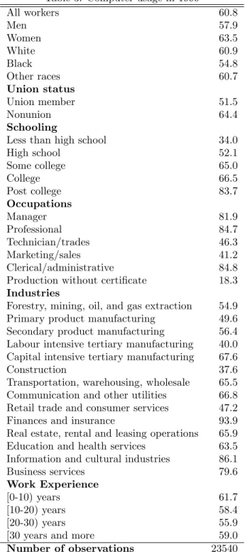
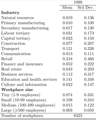
Table 3 shows the probability of computer use at work for various demo-graphic categories in 1999. Tables 4 and 5 provide descriptive statistics for employees and their workplaces, respectively. (It is not possible for con…den-tiality reasons to show minima and maxima.)
changes in computer use, considerably lower than they are in either Krueger (1993) or DiNardo and Pischke (1997). The simple explanation for this is that our data are much more recent.8 The patterns of computer use are extremely
similar in both countries. Females are more likely to use a computer than males, as are whites relative to blacks and nonunion members relative to union mem-bers. Computer use in both countries also rises monotonically with educational attainment. Computer use also varies considerably by occupation and industry as well as work experience.
4
Returns to Computer Use
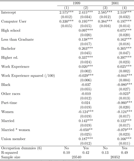
Table 6 presents Weighted Least Squares (WLS) estimates for the returns to computer use in 1999 and 2001. Our speci…cation as well as methodology mirrors Krueger (1993) to the extent possible. In columns 1 and 3, computer use is the only right hand side variable, while columns 2 and 4 correct for a number of worker characteristics.
Correcting for worker characteristics, the wage premium associated with computer use is just under 22 per cent, compared to Krueger’s 20 per cent estimate for 1989. This number is striking, especially given the high degree of penetration at the turn of the century. Our results are also otherwise remarkably similar to Krueger (1993)’s . In particular, wages are increasing in education and work experience (at a decreasing rate). They are lower (in 2001) for Blacks and Other races relative to Whites, as they are for Women relative to Men. Married men as well as Union members, by contrast, tend to have higher earnings. All of this suggests that our data are well-placed to analyze the question, …rst posed by Krueger, “Is the computer wage di¤erential real or illusory?”.9
8According to the 2001 Current Population Survey (CPS) –the data source used by Krueger
(1993) – computer use in the U.S. among the industries covered by WES was 54 per cent.
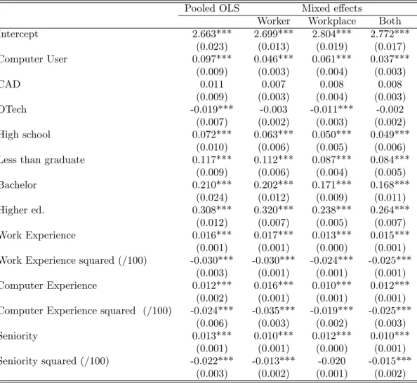
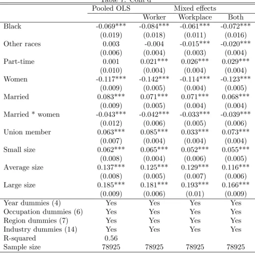
DiNardo and Pischke (1997)’s suggestion that the computer wage di¤erential may be illusory arises primarily from the problem of endogeneity in the form of omitted variables. In table 7 we begin to address this by including a number of additional, observable, worker and workplace characteristics, many of which Krueger (1993) was only indirectly able to control for.
In the interest of comparability, our speci…cation is constructed to mirror Entorf and Kramarz (1997) and Entorf, Gollac, and Kramarz (1999), who use French linked longitudinal employer-employee data of comparable structure to ours to examine the computer premium question.10 The pooled OLS results
pre-sented in Column 1 indicates that inclusion of these covariants, as anticipated, leads to a substantial reduction of the coe¢ cient on computer use from 0.197 to 0.097 –a number comparable to the coe¢ cient of 0.07 found by Entorf, Gollac, and Kramarz (1999) for France 7 years earlier. Our estimates also indicate that there exists a signi…cant premium associated with computer experience. Taking this into account suggests that, according to our pooled OLS estimates, the av-erage computer user (who has 6 years of computer experience) enjoys 19:2 per cent higher wages than non-users.
The pooled OLS estimator does not however correct for unobserved het-erogeneity, only yielding consistent estimates if there is no correlation between unobserved characteristics and right hand side variables. If it is the case, for in-stance, that more able workers are more likely to be assigned a computer or more likely to work at computer technology-intensive …rms, then this assumption will clearly be violated.
Columns 2-4 present the results of our mixed model, which corrects for unobserved heterogeneity while permitting for correlation between unobserved worker and workplace e¤ects with other covariates. Columns 2 and 3 correct
1 0The coe¢ cients on computer use and computer experience are robust to alternative
for worker and workplace e¤ects, respectively, while column 4 corrects for both. Once we correct for worker e¤ects, the coe¢ cient on computer use, pre-sented in column 2, drops from 0.097 to 0.046. This suggests that the worker selection e¤ect may account for roughly half of the observed computer wage premium. Interestingly, workplace e¤ects also bear considerable responsibility for the upward bias: correcting for this leads to an almost 40 per cent drop in the premium, from 0.097 to 0.061 (column 3).
Correcting for both worker and workplace in column 4 yields a premium to computer use of 3.8 per cent, compared to the 10.2 per cent observed in our pooled OLS estimates. If our estimates are indeed completely correcting for unobserved heterogeneity, then this may be interpreted as the productivity gain associated with providing a worker with a computer.
Interestingly, the coe¢ cient estimates pertaining to computer experience are not signi…cantly di¤erent once one moves from the pooled OLS to the full mixed model, suggesting that this variable is not unduely a¤ected by unobservable het-erogeneity. Taking into account the signi…cant returns associated with computer experience indicates that the average computer user (with 6 years of experience) earns a 13: 2 per cent higher wages than a non-user.
The size of the coe¢ cient in column 4 relative to those in columns 2 and 3 indicates that worker and workplace e¤ects are positively correlated. This is sug-gestive of positive sorting between workers and workplaces who, for unobserved reasons, are more likely to use computers. In other words, high ability workers, who are more likely to be assigned a computer, match with high productivity …rms which are more likely to invest in computers.
Although not the focus of this paper, it is worth noting that our results are in marked contrast to those of Entorf, Gollac, and Kramarz (1999), who …nd (in their Table 5) that correcting for individual and …rm …xed e¤ects yields
insignif-icant coe¢ cients on the computer use variable. Two obvious explanations are time and space. Our data are separated by 7 years, a period of time over which …rms were no doubt confronted with new developments in terms of complemen-tary innovations or cost reduction alternatives a¤ecting both IT adoption and worker productivity. Moreover, the data pertain to two di¤erent continents with di¤erent institutional structures governing both industry and labour.
Another explanation, however, lies in the fact that Entorf, Gollac, and Kra-marz (1999) use …xed e¤ects whereas we use mixed e¤ects. Fixed e¤ects models have a distinct advantage over mixed e¤ects to the extent that they do not im-pose additional distributional assumptions. However, since they are identi…ed via “switchers”, their coe¢ cient estimates tend to be imprecise over short pan-els with relatively little variation. This is certainly the case in our data. Our data follow workers for only 2 years, and when we estimate individual …xed ef-fects, our standard errors typically rise and our returns to computer use are not signi…cantly di¤erent from zero.11 Since Entorf, Gollac, and Kramarz (1999)
workers are followed for at most 3 years this is a problem which they must also, to some extent, face.
The main advantage of our mixed- over a …xed-e¤ects model it that it does not rely on “switchers” for identi…cation, thus yielding more precise estimates even with relatively short panels.12 Moreover, a comparison of coe¢ cients in
our mixed model and a model with …xed workplace e¤ects suggests similar implied biases relative to our pooled OLS estimates.13 Given that our …xed
workplace estimates are relatively more precise than our …xed worker estimates, given our longer (4 year) workplace panel, this suggests that the mixed model
1 1Fixed e¤ects estimation results are available from the authors upon request.
1 2Furthermore, the …xed e¤ects model relies upon the assumption that staying, leaving and
entering computer use each have the same e¤ect on wages. A simple test for this along the lines of Jakubson (1991) and Dolton and Makepeace (2004) leads to the rejection of this assumption for our data, suggesting that …xed e¤ects estimates would be biased in this context.
1 3In the workplace …xed e¤ects model, the implied bias is 9:7% 5:1% = 4:6% compared
does a rather good job of controlling for unobserved heterogeneity, at least at the workplace level. Finally, it should be noted that we can rely on another source of identi…cation when using workplace …xed e¤ects, namely variation in wages and computer use within the workplace.
5
Discussion
Is there a real computer wage di¤erential? We …nd that there is. The computer wage premium in our data is 3:8 per cent. In addition, the fact that there are signi…cant returns associated with computer experience means that the wage di¤erential between the average computer user and non-users is 13 per cent.
At the same time, DiNardo and Pischke (1997) were quite right to worry about the individual selection problem in estimating the computer wage pre-mium. Failure to correct for individual unobserved heterogeneity, results in an observed premium which is more than double the estimated 3:8 per cent.
We …nd that failure to correct for workplace e¤ects also results in a signif-icant overestimate of the computer wage premium. Although the literature to date has focused almost exclusively on worker e¤ects, this …nding need not be particularly surprising. Workplaces run by managers with high unobserved abil-ity, for instance, may be more likely to both invest in computers (especially if these are cost-cutting instruments) and have a relatively productive workforce. Alternatively, …rms operating in certain product markets may require both spe-cial skills (for which higher wages are paid) and relatively high computer use as a factor input.
The most natural stories which explain the mixed model estimates in our data involve high ability workers matching with high productivity …rms which are more likely to invest in computers. And this positive sorting, too, …nds support in our data, lending corroborative evidence to inter-industry studies
which have found that more computerised industries tend to employ more skilled (and presumably more able) workers (Berman, Bound, and Griliches (1994), Autor, Katz, and Krueger (1998) and Machin and Reenen (1998).)
The initial motivation behind Krueger’s study was to examine whether com-puters have changed the wage structure. It would be presumptuous at best to conclude, on the basis of our data, that they have. After all, according to our estimates, the returns to computer use are slightly smaller than those to having completed highschool, and nobody is arguing that a larger proportion of highschool graduates is what is driving rising wage inequality.
Nevertheless, the presence of a computer wage di¤erential, maintained in part by substantial returns to computer experience, may provide one possible explanation for why the U.S. and Canada have witnessed sustained wage in-equality through the turn of the century, at a time when the supply of college graduates seems to have levelled o¤ and the major skill-biased technological changes at the workplace are arguably well behind us.
References
Abowd, J. M. and F. Kramarz (1999a). The analysis of labor markets using matched employer-employee data. In O. Ashenfelter and D. Card (Eds.), Handbook of Labor Economics, Volume 3B, pp. 2629–2710. Elsevier Sci-ence, North-Holland.
Abowd, J. M. and F. Kramarz (1999b). Econometric analyses of linked employer-employee data. Labour Economics 6 (1), 53–74.
Acemoglu, D. (2002). Technical change, inequality and the labour market. Journal of Economic Literature 40 (1), 7–72.
today? evidence from german panel data. Labour 17 (3), 337–360. Autor, D. H., L. F. Katz, and A. B. Krueger (1998). Computing
inequal-ity: Have computers changed the labor market? Quarterly Journal of Economics 113 (4), 1169–1213.
Berman, E., J. Bound, and Z. Griliches (1994). Changes in the demand for skilled labor within U.S. manufacturing: Evidence from the annual survey of manufacturers. Quarterly Journal of Economics 109 (2), 367–397. DiNardo, J. E. and J.-S. Pischke (1997). The returns to computer use
revis-ited: Have pencils changed the wage structure too? Quarterly Journal of Economics 112 (1), 291–303.
Dolton, P. and G. Makepeace (2004). Computer use and earnings in britain. The Economic Journal 114 (1), C117–C129.
Entorf, H., M. Gollac, and F. Kramarz (1999). New technologies, wages, and workers selection. Journal of Labor Economics 17 (3), 464–491.
Entorf, H. and F. Kramarz (1997). Does unmeasured ability explain the higher wages of new technology workers? European Economic Review 41, 1489– 1509.
Jakubson, G. H. (1991). Estimation and testing of the union wage e¤ect using panel data. Review of Economic Studies 58, 971–991.
Krueger, A. B. (1993). How computers have changed the wage structure: Evidence from microdata. Quarterly Journal of Economics 108 (1), 33– 60.
Machin, S. and J. V. Reenen (1998). Technology and changes in skill struc-ture: Evidence from seven OECD countries. Quarterly Journal of Eco-nomics 113, 1215–1244.
Table 1: Movers versus Stayers
Computer Use 1999 only 1999-2000 Total
# % # % #
No 1463 0.43 6084 0.30
One period only 1910 0.57 2188 0.11
Both periods 11895 0.59
Total 3373 1.00 20167 1.00 23540
Computer Use 2001 only 2001-2002
# % # % #
No 1458 0.41 5161 0.31
One period only 2081 0.59 1910 0.11
Both periods 9742 0.58
Total 3539 1.00 16813 1.00 20352
Table 2: Stay, Leave and Enter Computer Use 1999-2000 or 2001-2002 # % Stay 21637 0.59 Leave 1200 0.03 Enter 1849 0.05 None 11245 0.31 Total 35931 1.00
Table 3: Computer usage in 1999 All workers 60.8 Men 57.9 Women 63.5 White 60.9 Black 54.8 Other races 60.7 Union status Union member 51.5 Nonunion 64.4 Schooling
Less than high school 34.0
High school 52.1 Some college 65.0 College 66.5 Post college 83.7 Occupations Manager 81.9 Professional 84.7 Technician/trades 46.3 Marketing/sales 41.2 Clerical/administrative 84.8
Production without certi…cate 18.3 Industries
Forestry, mining, oil, and gas extraction 54.9 Primary product manufacturing 49.6 Secondary product manufacturing 56.4 Labour intensive tertiary manufacturing 40.0 Capital intensive tertiary manufacturing 67.6
Construction 37.6
Transportation, warehousing, wholesale 65.5 Communication and other utilities 66.8 Retail trade and consumer services 47.2
Finances and insurance 93.9
Real estate, rental and leasing operations 65.9 Education and health services 63.5 Information and cultural industries 86.1
Business services 79.6
Work Experience
[0-10) years 61.7
[10-20) years 58.4
[20-30) years 55.9
[30 years and more 59.0
Table 4: Descriptive statistics - Employees
1999 2001
Mean Std Dev Mean Std Dev
ln(hourly wage) 2.778 0.521 2.820 0.530
Highest completed degree
Less then high school 0.107 0.309 0.120 0.325
High school 0.175 0.380 0.179 0.384
Industry training 0.053 0.162 0.033 0.365
Trade or vocational diploma 0.088 0.283 0.098 0.297
Some college 0.104 0.305 0.108 0.310 Completed college 0.181 0.385 0.188 0.391 Some university 0.077 0.266 0.067 0.249 Teacher’s college 0.002 0.049 0.001 0.030 University certi…cate 0.018 0.132 0.020 0.138 Bachelor degree 0.130 0.337 0.133 0.339
University certi…cate (> bachelor) 0.019 0.135 0.015 0.120
Master’s degree 0.031 0.174 0.028 0.165
Degree in medicine, dentistry, etc. 0.008 0.092 0.007 0.085
Earned doctorate 0.006 0.078 0.005 0.067
Seniority (years) 8.517 8.206 8.518 8.206
Work Experience (years) 16.167 10.714 16.411 10.993
Black 0.011 0.104 0.014 0.119 Other races 0.280 0.449 0.309 0.462 Women 0.521 0.500 0.506 0.500 Married 0.566 0.496 0.541 0.498 Computer user 0.608 0.488 0.601 0.490 CAD 0.120 0.325 0.133 0.340 Otech 0.269 0.443 0.228 0.420
Computer Experience (years) 5.865 6.373 6.483 6.732
Union member 0.279 0.449 0.280 0.449 Part-time 0.051 0.220 0.053 0.224 Occupations Manager 0.151 0.358 0.112 0.315 Professional 0.162 0.368 0.175 0.380 Trader/Technician 0.390 0.488 0.414 0.493 Marketing/sales 0.084 0.277 0.085 0.279 Clerical/administrative 0.140 0.347 0.137 0.344 Production w/o certi…cate 0.074 0.262 0.077 0.267
Table 5: Descriptive statistics - Workplaces 1999 Mean Std Dev. Industry Natural resources 0.019 0.136 Primary manufacturing 0.010 0.100 Secondary manufacturing 0.017 0.130 Labour tertiary 0.031 0.173 Capital tertiary 0.023 0.150 Construction 0.077 0.267 Transport 0.121 0.326 Communication 0.013 0.111 Retail 0.318 0.466
Finance and insurance 0.052 0.222
Real estate 0.043 0.203
Business services 0.112 0.317
Education and health services 0.141 0.348 Culture and information 0.022 0.147 Workplace size Tiny (1-9 employees) 0.874 0.331 Small (10-99 employees) 0.108 0.310 Medium (100-499 employees) 0.015 0.122 Large (>500 employees) 0.003 0.050 Number of workplaces: 6322
Table 6: Impact of Computer Use in Basic Linear Models 1999 2001 (1) (2) (3) (4) Intercept 2.575*** 2.415*** 2.585*** 2.519*** (0.012) (0.034) (0.012) (0.032) Computer User 0.330*** 0.195*** 0.384*** 0.197*** (0.015) (0.015) (0.016) (0.014) High school 0.097*** 0.075*** (0.020) (0.020)
Less than Graduate 0.138*** 0.162***
(0.017) (0.018) Bachelor 0.263*** 0.305*** (0.045) (0.047) Higher ed. 0.337*** 0.397*** (0.024) (0.023) Work Experience 0.020*** 0.025*** (0.002) (0.002)
Work Experience squared (/100) -0.029*** -0.044***
(0.006) (0.004) Black -0.037 -0.080*** (0.055) (0.027) Other races -0.010 -0.023* (0.012) (0.013) Part-time 0.024 -0.060*** (0.019) (0.020) Women -0.124*** -0.124*** (0.019) (0.017) Married 0.142*** 0.122*** (0.019) (0.017) Married * women -0.050** -0.079*** (0.025) (0.023) Union member 0.187*** 0.166*** (0.012) (0.011)
Occupation dummies (6) No Yes No Yes
R-squared 0.10 0.42 0.13 0.49
Sample size 23540 20352
Statistical signi…cance: *=10%; **=5%; ***=1% Robust standard errors in parentheses.
Table 7: Impact of Computer Use in OLS and Mixed-E¤ects Models
Pooled OLS Mixed e¤ects
Worker Workplace Both
Intercept 2.663*** 2.699*** 2.804*** 2.772*** (0.023) (0.013) (0.019) (0.017) Computer User 0.097*** 0.046*** 0.061*** 0.037*** (0.009) (0.003) (0.004) (0.003) CAD 0.011 0.007 0.008 0.008 (0.009) (0.003) (0.004) (0.003) OTech -0.019*** -0.003 -0.011*** -0.002 (0.007) (0.002) (0.003) (0.002) High school 0.072*** 0.063*** 0.050*** 0.049*** (0.010) (0.006) (0.005) (0.006)
Less than graduate 0.117*** 0.112*** 0.087*** 0.084***
(0.009) (0.006) (0.004) (0.005) Bachelor 0.210*** 0.202*** 0.171*** 0.168*** (0.024) (0.012) (0.009) (0.011) Higher ed. 0.308*** 0.320*** 0.238*** 0.264*** (0.012) (0.007) (0.005) (0.007) Work Experience 0.016*** 0.017*** 0.013*** 0.015*** (0.001) (0.001) (0.000) (0.001) Work Experience squared (/100) -0.030*** -0.030*** -0.024*** -0.025***
(0.003) (0.001) (0.001) (0.001)
Computer Experience 0.012*** 0.016*** 0.010*** 0.012***
(0.002) (0.001) (0.001) (0.001) Computer Experience squared (/100) -0.024*** -0.035*** -0.019*** -0.025***
(0.006) (0.003) (0.002) (0.003)
Seniority 0.013*** 0.010*** 0.012*** 0.010***
(0.001) (0.001) (0.000) (0.001) Seniority squared (/100) -0.022*** -0.013*** -0.020 -0.015***
Table 7: Cont’d
Pooled OLS Mixed e¤ects
Worker Workplace Both
Black -0.069*** -0.084*** -0.061*** -0.072*** (0.019) (0.018) (0.011) (0.016) Other races 0.003 -0.004 -0.015*** -0.020*** (0.006) (0.004) (0.003) (0.004) Part-time 0.001 0.021*** 0.026*** 0.029*** (0.010) (0.004) (0.004) (0.004) Women -0.117*** -0.142*** -0.114*** -0.123*** (0.009) (0.005) (0.004) (0.005) Married 0.083*** 0.071*** 0.071*** 0.068*** (0.009) (0.005) (0.004) (0.004) Married * women -0.043*** -0.042*** -0.033*** -0.039*** (0.012) (0.006) (0.005) (0.006) Union member 0.063*** 0.085*** 0.033*** 0.073*** (0.007) (0.004) (0.004) (0.004) Small size 0.062*** 0.065*** 0.052*** 0.055*** (0.008) (0.004) (0.006) (0.005) Average size 0.137*** 0.125*** 0.129*** 0.116*** (0.008) (0.005) (0.007) (0.006) Large size 0.185*** 0.181*** 0.193*** 0.166*** (0.009) (0.006) (0.01) (0.009)
Year dummies (4) Yes Yes Yes Yes
Occupation dummies (6) Yes Yes Yes Yes
Region dummies (7) Yes Yes Yes Yes
Industry dummies (14) Yes Yes Yes Yes
R-squared 0.56
Sample size 78925 78925 78925 78925
Statistical signi…cance: *=10%; **=5%; ***=1%. Robust standard errors in parentheses.
A
Appendix: Estimation
REML methods involve applying maximum likelihood (ML) to linear functions of y, i.e. K0y (McCulloch and Searle (2001)). Note that K0 is speci…cally
designed so that K0y contains none of the …xed e¤ects ( and in our case)
which are part of the model for y. Thus, REML is simply ML applied on K0y
and can be interpreted as maximizing a marginal likelihood.
Each vector of K is chosen so that k0y = 0 or K0[X U ] = 0. With
y s N(X + U ; V ) it follows that
K0y s N(0; K0V K),
where V = DD0 2 + F F0 2 + is the covariance of earnings implied by the
assumptions we made about the distribution of the unobserved heterogeneity terms. The REML log-likelihood is therefore
log LREM L= 1 2(N r) log 2 1 2log jK 0V Kj 1 2y 0K(K0V K) 1K0y. (1)
There are two advantages of using REML. First, variance components are esti-mated without being a¤ected by the …xed e¤ects. This means that the variance estimates are invariant to the values of the …xed e¤ects. Second, in estimating variance components with REML, degrees of freedom for the …xed e¤ects are taken into account implicitly whereas with ML they are not.1 Both methods
have the same merits of being based on the maximum likelihood principle and parameter estimates inherit the consistency, e¢ ciency, asymptotic normality and invariance properties that follow.
Maximization of the likelihood function (1), while providing us with
esti-1REML estimates are also invariant to whatever set of contrasts is chosen for K0yas long
mates for the variance components, will not yield estimates for the random and …xed e¤ects. In a second step, we obtain estimates for the random and …xed ef-fects using a set of equations developed by Henderson, Kempthorne, Searle, and Krosigk (1959). These equations have become known as Henderson’s Mixed Model Equations (MME) and simultaneously yield the Best Linear Unbiased Estimates (BLUE) of the …xed e¤ects and Best Linear Unbiased Predictors (BLUP) of the random e¤ects for known values of the variance components and
2. De…ne the matrix of variance components as
= 2 6 4 2I N 0 0 2I J 3 7 5 : (2)
For the particular structure implied by the model, the MME are 2 6 6 6 6 6 6 6 6 4 2 6 4 X 0 U0 3 7 5 1[X U ] 2 6 4 X 0 U0 3 7 5 1[D F ] 2 6 4 D 0 F0 3 7 5 1[X U ] 2 6 4 D 0 F0 3 7 5 1[D F ] + 1 3 7 7 7 7 7 7 7 7 5 2 6 6 6 6 6 6 6 4 ^ ^ ^ ^ 3 7 7 7 7 7 7 7 5 = = 2 6 6 6 6 6 6 6 6 4 2 6 4 X 0 U0 3 7 5 1y 2 6 4 D 0 F0 3 7 5 1y 3 7 7 7 7 7 7 7 7 5 : (3)
Estimates for and are obtained from the REML step.
2BLUE and BLUP estimates make us feel quite con…dent that a full information approach
would not yield any better (in the sense of lower variance) estimator, although it might if we were to use a di¤erent class of estimators.
References
Henderson, C., O. Kempthorne, S. Searle, and C. Krosigk (1959). The estima-tion of environmental and genetic trends from records subject to culling. Biometrics 15 (2), 192–218.
McCulloch, C. and S. Searle (2001). Generalized, Linear and Mixed Models. Wiley Series in Probability and Statistics, John Wiley and Sons Inc. Searle, S. R., G. Casella, and C. McCulloch (1992). Variance Components.