Spectroscopic investigation of arc over an ice surface

UNIVERSITE DU QUÉBEC

THESE PRESENTEE A

L'UNIVERSITÉ DU QUÉBEC À CHICOUTIMI

COMME EXIGENCE PARTIELLE

DU DOCTORAT EN INGÉNIERIE

par

AZAM NEKAHI

ETUDE SPECTROSCOPIQUE DE L'ARC A LA

SURFACE DE LA GLACE

SPECTROSCOPIC INVESTIGATION OF ARC OVER

AN ICE SURFACE

ABSTRACT

Ice accumulation on insulators of overhead transmission lines and substations has been recognized as a major problem which may cause insulator flashover and power outages. This phenomenon starts with corona discharge activity and continues with the formation of partial arcs which may result in flashover. Due to the complexity of the process, resulting from surface interaction of discharge with the water film on the ice surface, is not yet fully understood. As for any other type of discharge, the knowledge of some parameters such as temperature and concentration of different species is necessary in order to describe the mechanisms involved. Moreover, to develop mathematical models for discharge propagation, an estimation of discharge channel conductivity is necessary. The current flows through this conductive channel and supplies the energy needed to sustain the ionization activity inside the channel. The conductivity of discharge channel is directly related to its temperature, which illustrates the need for discharge temperature measurements. Up to now, for an arc over an ice surface the temperature has been assumed to have a constant value of 5,000 K, but without any experimental support. The existence of Local Thermodynamic Equilibrium (LTE) is another important aspect for proposing theories and models, but this has not yet been verified for flashover on ice-covered insulators. The verification of LTE condition requires information about temperature and concentration of different species, electron density and ionization level.

The objective of this research is to augment our knowledge of flashover on ice-covered insulators by measuring and calculating several important discharge column parameters. Measurement of rotational and excitation temperatures, and electron density during arc propagation are the first steps. The effect of discharge current, voltage type

and polarity on the variation of the mentioned arc parameters should be also studied. Based on these data, the LTE condition could be examined.

Spectroscopic plasma diagnostic is a non-destructive test method used to achieve the stated objectives. The emitted light from an arc over an ice surface was transmitted to a spectrometer. The time-resolved recorded spectra of arc were used to study the nature and concentration of ionized species. The gas and electron temperatures and electron densities were also measured using Boltzmann and Stark broadening methods.

Measured rotational temperatures were found to vary from 4,000 K to 6,500 K, while the current increased from 200 mA to 700 mA during the discharge propagation. It was observed that under similar experimental conditions, the arc current intensity of DC+ arcs were hotter than that of DC-. Moreover, arc temperatures under AC voltage were lower than those of DC+, and close to that of DC-. The excitation temperature was measured at about 9,000 K and does not vary significantly with discharge current. As current increases, electron densities increased as well. For currents ranging from 200 mA to 700 mA, electron densities increased from 1 to 2 xio17 cm'3. Electron densities increased up to 2.5xlO17 cm"3 at the later stages of arc development, when flashover occurs. Differences between the rotational and excitation temperatures showed that the arc was not in a state of thermal equilibrium.

RESUME

L'accumulation de glace sur les isolateurs de lignes de transport d'énergie électrique et de leurs postes est reconnue comme un problème majeur qui peut causer le contoumement des isolateurs et dans certaines conditions l'interruption de courant. Ce phénomène commence par des activités de décharge de couronne, s'ensuit la formation d'arcs partiels qui peut se développer en arcs de contoumement. Dû à la complexité de ce processus, qui résulte de l'interaction des décharges avec le film d'eau formé à la surface de la glace, le phénomène de contoumement n'est pas encore entièrement compris. Pour une meilleure connaissance des mécanismes en jeu dans l'arc de contoumement et d'autres types de décharge le précédant, il sera nécessaire de développer certaines connaissances concernant des paramètres comme la température et la concentration d'autres espèces d'ions. De plus, afin de développer des modèles mathématiques pour la propagation de décharges, une estimation de la conductivité de canal de décharge est nécessaire. Le courant circulant dans ce canal conducteur fournit l'énergie nécessaire aux activités d'ionisation à l'intérieur de ce canal. La conductivité de ce dernier est une fonction directe de sa température, ce qui illustre le besoin de mesurer la température de ces décharges. Jusqu'à présent, pour un arc apparaissant le long d'une surface de glace, on a arbitrairement donné à cette température a une valeur de 5000 K, mais sans preuve expérimentale. L'existence d'équilibre thermodynamique local (ETL) est un autre aspect important pour proposer des théories et des modèles, mais ceci n'a pas été vérifié pour l'arc de contoumement sur les isolateurs recouverts de glace. La vérification de condition d'ETL exige des informations sur la température et la concentration de diverses espèces ioniques, ainsi que sur la densité d'électron et sur le degré d'ionisation.

L'objectif principal de cette recherche est d'approfondir nos connaissances du contournement des isolateurs recouverts de glace en mesurant et en calculant plusieurs paramètres importants dans le canal de décharge. La mesure des températures rotationnelles et d'excitation, et de la densité d'électrons pendant la propagation d'arc est préalablement nécessaire. De plus, l'effet du courant de décharge, du type de tension et de sa polarité sur la variation des paramètres d'arc ci-haut mentionnés devrait être étudié. Sur les bases de ces données, la condition d'ETL pourrait être examinée.

Le diagnostic spectroscopique de plasma est une méthode de test non destructive qui a été utilisée pour atteindre les objectifs mentionnés. La lumière émise d'un arc sur une surface de glace a été transmise à un spectromètre. Les spectres obtenus ont été utilisés pour étudier la nature et la concentration d'espèces d'ions. Les températures du gaz et des électrons, ainsi que leur densité, ont été également mesurées à l'aide de méthodes appropriées.

Les températures rotationnelles mesurées se situaient entre 4000 et 6500 K, alors que l'intensité de courant a augmenté de 200 à 700 mA pendant la propagation des décharges. Il a été observé que dans les mêmes conditions expérimentales, les températures des arcs en courant continu positif étaient plus élevée que celle des arcs en courant continu négatif. De plus, les températures d'arc en courant alternatif étaient plus faible que celles en courant continu positif et prohes de celles en courant continu négatif. La température d'excitation mesurée se situait à environ 9000 K et ne variait pas signifïcativement en fonction du courant de décharge. La densité d'électron augmentait avec l'augmentation du courant. Pour les courants variant de 200 à 700 m A, les densités d'électron ont augmenté de 1 à 2 xlO17 cm"3. Les densités d'électron étaient supérieures à 2.5xlO17 cm"3 avant l'apparition de l'arc de contournement. Les différences entre les

températures rotationnelles et d'excitation ont montré que l'arc n'était pas dans un état d'équilibre thermique.

ACKNOWLEDGMENTS

This work was carried out within the framework of the NSERC/Hydro-Quebec/UQAC Industrial Chair on Atmospheric Icing of Power Network Equipment (CIGELE) and the Canada Research Chair on Atmospheric Icing Engineering of Power Networks (INGIVRE) at Université du Québec à Chicoutimi (UQAC). I would like to thank the CIGELE partners (Hydro-Québec, Hydro One, Réseau Transport d'Électricité (RTE) and Électricité de France (EDF), Alcan Cable, K-Line Insulators, Tyco Electronics, Dual-ADE, CQRDA, and FUQAC) whose financial support made this research possible.

I would like to express my gratitude to my supervisor, Professor Masoud Farzaneh, whose expertise, understanding, and patience, added considerably to my graduate experience. I appreciate his vast knowledge and skill in many areas.

Many thanks go in particular to Dr. W.A. Chisholm for his valuable advice and discussion.

I would like to extend my thanks to Marc André Perron, Xavier Bouchard, Pierre Camirand, and Claude D'Amours at CIGELE Laboratory for their technical support and to Denis Masson and Désirée Lezou for their help with administrative tasks.

I am very grateful to Jean Talbot for his precious efforts and editorial help for making this thesis legible.

Most importantly, I would like to thank all my friends who helped me get through the years of my study.

This thesis is dedicated to my parents, who taught me the value of education, to my mother so far away who has inspired me profoundly. To my father who has constantly encouraged me to reach my dreams. I am deeply indebted to them for their continued support and unwavering faith in me.

I am grateful to my husband, Shahab for his constant love and strength throughout the years. Without him, and his ability to raise my spirits when I was most discouraged, I could never made it this far. Above all and the most needed, he provided me encouragement and support in various ways. Shahab, you were the wind beneath my

wing and of course to my little Najin, who was like a star guiding me through the nights during my intense work.

TABLE OF CONTENTS

ABSTRACT 2 RÉSUMÉ 4 ACKNOWLEDGMENTS 7 LIST OF FIGURES 12 LIST OF TABLES 14 CHAPTER 1 15 INTRODUCTION 15 1.1 Overview 16 1.2 Research objectives 18 1.3 Statement of originality and contribution to knowledge 20 1.4 Methodology 20 1.4.1 Rotational temperature measurements 21 1.4.2 Excitation temperature measurements 21 1.4.3 Electron density measurements 22 1.5 Structure of the thesis 22 CHAPTER 2 23 LITERATURE REVIEW 23 2.1 Introduction 24 2.2 Plasma 25 2.3 Spectroscopic plasma diagnostics 26 2.3.1 Mechanism of emission and absorption of spectra 27 2.3.2 Different types of emission spectra 30

2.3.2.1 Line spectra 30 2.3.2.2 Continuum spectra 31 2.3.2.3 Line profiles 32 2.3.2.4 Band spectra 32

2.4 Spectroscopic temperature measurement techniques 32 2.4.1 Rotational temperature measurement 33 2.4.2 Excitation temperature measurement 35 2.5 Spectroscopic density measurement techniques 39 2.6 Arc discharge temperature and electron density measurement 43 2.7 Thermodynamic study of plasma 46 2.7.1 Thermal equilibrium in the arc 46

2.7.1.1 Maxwell's Law 47 2.7.1.2 Plank's Law 47 2.7.1.3 Saha's equation 49 2.7.1.4 Boltzmann's Law 49 2.7.1.5 Partition function 50 2.8 Thermodynamic equilibrium 51 2.8.1 Thermodynamic properties 52 2.8.1.1 Mass density 52 2.8.1.2 Enthalpy 52

2.8.1.3 Heat Capacity at constant pressure 53 2.8.2 Composition and thermodynamic properties of two-temperature plasma.. 53 2.8.3 Local Thermodynamic Equilibrium 54 2.8.3.1 Criteria for Local Thermodynamic Equilibrium 56 2.8.3.2 Partial Local Thermodynamic Equilibrium 57 2.9 Conclusion 60 CHAPTER 3 61 METHODOLOGY AND EXPERIMENTAL PROCEDURE 61 3.1 Introduction 62 3.2 Equipment and facilities 62 3.2.1 High-voltage system 63 3.2.2 Climate room 64 3.2.3 Spectroscopic system 64 3.2.4 Data acquisition system 66 3.3 Experimental procedure 66 3.3.1 Setup 66 3.3.2 Calibration 68 3.3.3 Current and voltage measurements 69 3.3.4 Rotational temperature measurements 71 3.3.5 Excitation temperature measurements 72 3.3.6 Electron density measurements 74 3.3.7 Local Thermodynamic Equilibrium 75 3.4 Conclusion 76 CHAPTER 4 77 EXPERIMENTAL RESULTS 77 4.1 Introduction 78 4.2 Identified spectral lines and bands 78 4.3 Gas temperature measurements 81 4.3.1 AC applied voltage 81 4.3.2 DC applied voltage 86 4.3.2.1 DC- 86 4.3.2.2 DC+ 91 4.4 Excitation temperature 91 4.5 Electron density measurement 99 CHAPTER 5 108 DISCUSSIONS ON RESULTS 108 5.1 Introduction 109 5.2 Excitation reactions 109 5.2.1 N2+ first negative system 109 5.2.2 OI lines 110 5.2.3 N a - D lines I l l 5.2.4 NHband I l l 5.2.5 OH band 112 5.3 Overall spectral variation of arc 112 5.4 Voltage polarity effect 117 5.5 Error analysis 120 5.6 Verifying thermal equilibrium 121

5.7 Conclusion 123 CHAPTER 6 124 CONCLUSIONS AND RECOMMENDATIONS 124 6.1 Conclusions 125 6.2 Recommendations for future work 129 CHAPTER 7 131 REFERENCES 131

LIST OF FIGURES

Figure 2.1. Excitation levels of an atom or an ion [10] 29 Figure 2.2. Energy curves for a diatomic molecule (CN) and schematic spectrum of the

violet and red systems [10] 30 Figure 2.3. Gas and electron temperature and ionization degree in the leader channel,

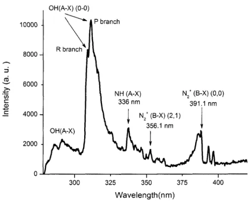
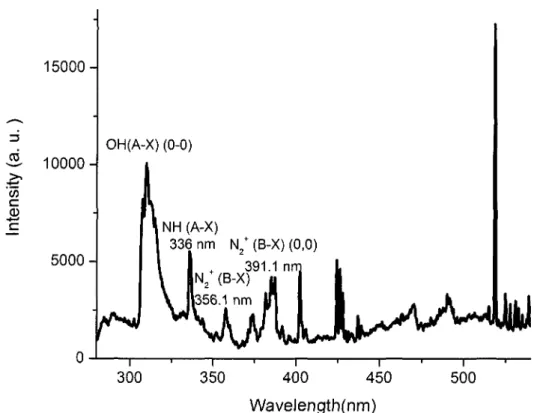
comparison of Les Renardières Group [52] results with Orville [49] and Vassy [53] 44 Figure 2.4. Plank's distribution 48 Figure 2.5. Scheme of levels [10] 58 Figure 3.1. Triax 320 top view [68] user's manual 65 Figure 3.2. Ice geometry 67 Figure 3.3. Schematic diagram of the experimental setup 68 Figure 3.4. Setup arrangement to measure AC voltage and current 70 Figure 3.5. Setup arrangement to measure DC voltage and current 70 Figure 4.1. Identified bands from a typical spectrum of light emitted from DC discharge

for the region between 280 nm and 420 nm 79 Figure 4.2. Identified lines from a typical spectrum of light emitted from DC discharge

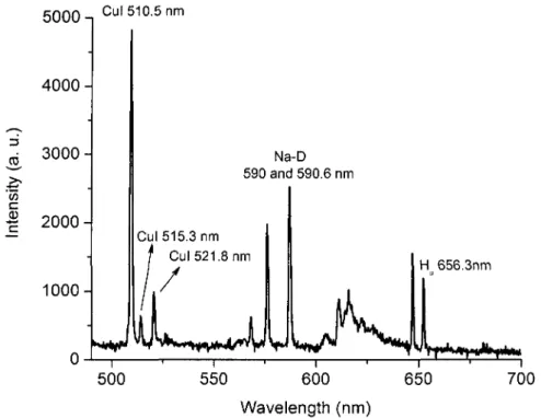
for the region between 500 nm and 700 nm 80 Figure 4.3. Identified lines from a typical spectrum of light emitted from DC discharge

for the region between 750 nm and 1000 nm 81 Figure 4.4. Spectrum of a discharge during its development over the ice surface 82 Figure 4.5. Spectrum of an arc during the final jump (which leads to flashover) 82 Figure 4.6. Emission intensity variation of peak intensities of OH (A-X) at 309 nm, NH

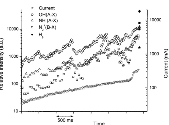
(A-X) at 336 nm, N2+ (B-X) at 391.1 nm, and Hp at 486 nm. Measurement points at the end emphasized with filled shapes correspond to the flashover instant. The variation of the RMS value of AC current has also been

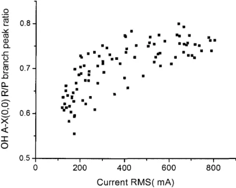
depicted 83 Figure 4.7. Current waveform profile used for rotational temperature measurements 84 Figure 4.8. Ratios of peak intensities of the OH (0, 0) R and P branches as a function of

RMS value of current during each spectrum acquisition (8ms) 85 Figure 4.9. Simulated ratio of peak intensities of the OH (0, 0) R and P branches relative

to rotational temperatures. These simulations were performed with

SPECAIR [8] software 85 Figure 4.10. Evolution of gas temperatures during the AC discharge obtained from the

rotational temperatures of OH emission bands calculated by ratio of peak intensities of the OH (0, 0) R and P branches 86 Figure 4.11. The profile of recorded spectra during discharge development 88 Figure 4.12. Current variation during discharge development leading to flashover 88 Figure 4.13. Experimental spectra recorded for 228 mA and 765 mA discharges, and

synthetic spectra of OH A-X (0,0) emissions simulated for different

rotational temperatures 89 Figure 4.14. Rotational temperature measurements using UV-OH (A-X) for a

Figure 4.15. Experimental spectrum recorded for 1,000 mA discharge and synthetic spectra of the N2+ 1st negative system simulated for different rotational temperatures

90 Figure 4.16. Evolution of gas temperatures during DC+ discharge obtained from the

rotational temperatures of OH emission bands calculated by ratio of peak intensities of the OH (0, 0) R and P branches 91 Figure 4.17. Time resolved spectra of the arc over an ice surface a) between 775 nm and

1,000 nm b) between 505 nm and 525 nm 92 Figure 4.18. A typical Boltzmann plot using the copper line parameters found in Table

4.1, for a 485 mA discharge current 95 Figure 4.19. Excitation temperature using copper lines versus discharge current 95 Figure 4.20. A typical Boltzmann plot using the parameters found in Table 4.2 for singly

ionized oxygen lines, for a 449 mA discharge current 96 Figure 4.21. Oxygen excitation temperature variations relative to discharge current 96 Figure 4.22. Reconstructed Boltzmann plot using the Burton and Blades correction

parameter for copper lines, for a 485 mA discharge current 98 Figure 4.23. Excitation temperatures of copper using the Burton and Blades correction

parameter at different discharge currents 99 Figure 4.24. Time-resolved spectra during discharge development 100 Figure 4.25. Current variations during discharge development 101 Figure 4.26. Haline profiles relative to time 101 Figure 4.27. Dotted lines: Normalized Stark profiles of Ha lines for different electron

densities at Te =10,000 K, from the data provided by Griem [42]. Solid lines: Results of convolution of Griem data with measured instrumentation function 102 Figure 4.28. Spectrum at 615 mA, background continuum level and subtracted profile 103 Figure 4.29. Comparison of the normalized measured and theoretical Ha line profiles at

615 mA. The theoretical profile given by Griem [42] is for an electron density of 1.64xl017cm"3 103 Figure 4.30. FWHM of profiles for different electron densities, considering the measured

instrumentation broadening 104 Figure 4.31. Variation of FWHM of Ha line with arc current 106 Figure 4.32. Variation of electron density with arc current during propagation 106 Figure 5.1. Spectra of arc light during (a) white arc 250-500 nm (b) white arc 500-750 nm (c) fiashover arc 250-500 nm and (d) flashover arc 500-750nm 115

Figure 5.2. Time-resolved spectra of white arc 116 Figure 5.3. Time-resolved spectra of arc at different stages 116 Figure 5.4. Rotational temperatures versus current for different applied voltage types. 117 Figure 5.5. The voltage gradient along arc column versus current for different applied

voltage types (adapted from data of [83,84]) 119 Figure 5.6. Power loss per arc length along arc column versus current for different

applied voltage types 120 Figure 5.7. Comparison of excitation and rotational temperatures 123

LIST OF TABLES

Table 2.1. Spectra observed in plasma [10] 28 Table 3.1. Table Spectroscopic parameters of copper spectral lines 72 Table 4.1. Spectroscopic parameters of copper spectral lines [74] 93 Table 4.2. Spectroscopic parameters of oxygen spectral lines [74] 93 Table 5.1. Typical values^ of A and n in relation E=AFn for arcs over an ice surface [83, 84] 118

CHAPTER 1

INTRODUCTION

CHAPTER 1

INTRODUCTION

1.1 Overview

In cold climate regions, ice accretion on outdoor insulators may cause a drastic reduction of their electrical insulation strength, sometimes resulting in flashovers and power outages [1]. Incidents caused by flashover on ice-covered insulators have been reported by various authors from different countries [2- 4].

The electric field along an insulator is non-uniform. In the high stress areas of the insulator, partial discharges and arcs can lead to ice shedding. This will cause some part of the insulator string to become ice free; these ice-free zones are referred to as air gaps. The formation of a water film on the ice surface is the first step of this process. This film can be formed by a rise in ambient temperature, sunshine, condensation, the heating effect of electrical discharge, or leakage current. Because of the high conductivity of the water film, leakage resistance is decreased and voltage drops are observed across the air gaps. The high electric field will initiate corona discharges, leading to the development of local arcs at this area. This will cause an increase in leakage current and consequent ice melting. If the leakage current continues to increase over a short period, a white arc will appear, which will accelerate ice melting and cause further increase in leakage current.

When the length of arc reaches about 60% of inter-electrode distance, the speed of arc propagation will increase rapidly, leading to flashover of the whole insulator string [2].

Considerable efforts have been made to develop dynamic and static mathematical models for studying the propagation of the arc over an ice surface [5, 6] and predicting the critical flashover voltage of ice- or snow-covered insulators.

The formation of a flashover arc on an ice surface is a complex process and is not fully understood. Many researchers have tried to characterize arcing by determining the arc constants using a relationship between arc voltage and current. However, very little has been done in terms of determining arc temperature, which is an important component of flashover modeling [7].

In order to simulate arc propagation, initial values of different circuit elements in each stage of propagation are required. In the existing dynamic models, the exact values of the different variables, such as arc length and temperature, and surface condition, are required for simulating the arc current. Otherwise, the prediction of arc current during propagation cannot be carried out [7]. Concerning arc temperature, it has been assumed, without any experimental support, to have a constant value of 4,550 K during white arc propagation.

Also, rotational temperature, which is close to gas temperature [8], should be determined and compared to the electronic temperature in order to verify the existence of Local Thermodynamic Equilibrium (LTE) [9].

Moreover, no data are available to calculate the electron density of arc on an ice surface, which is an important parameter for understanding the flashover mechanisms as well for evaluating the existence of LTE.

Spectroscopic plasma diagnostic methods provide some important advantages of interest to researchers for a long time. This technique enables to obtain a large amount of information about plasma without disturbing it. In addition, it is applicable to transient as well as to stationary states [10, 11].

Luminous emissions from arcs and plasmas often have complex spectral structures. Line spectra, particularly if time-resolved, can yield much information not only on the nature and concentration of ionized species, but also on the gas and electron temperatures, and electron density [12]. The spectroscopic investigation of discharge can also provide insights on the physics of ice surface discharge.

The main purpose of this project is to carry out a spectroscopic analysis of arcs formed on the surface of ice to determine their rotational and excitation temperatures, and also their electron densities. The results will be used to verify the existence of LTE in the discharge channel.

1.2 Research objectives

The main objective of this thesis is the spectroscopic investigation of arcs formed over an ice surface. This comprises the two following stages: identifying the different lines in the arc spectra, and calculating arc temperatures and electron densities.

The specific objectives are:

• Identifying the lines and bands specific to various atoms and molecules Detailed analyses of the spectra allow identifying different atomic lines and molecular bands from background gases, as well as excited species from polluted ice.

• Developing a method for the measurement of gas and excitation

temperatures of arcs formed over an ice surface

Optical emission spectroscopy is an applicable method for the measurement of excitation and rotational temperatures of this type of discharge.

• Developing a method for electron density measurement of arcs formed over an ice surface

Some spectral lines are broadened under the effect of the electric field resulting from the concentration of free-electrons. The Stark broadening method can be used to obtain the electron density of the arc channel.

• Investigating the variation of gas and excitation temperatures, and electron densities of arcs over an ice surface at different current levels during arc

propagation

Time-resolved spectra will be recorded and analyzed to obtain the gas and excitation temperatures, and electron densities. When combined with synchronized electrical measurements these data should yield the overall variation of the measured quantities with the discharge current during arc propagation.

• Examining the existence of LTE in the discharge channel

Based on the results of the temperature and electron density measurements of different species, the existence of thermodynamic equilibrium will be examined.

1.3 Statement of originality and contribution to

knowledge

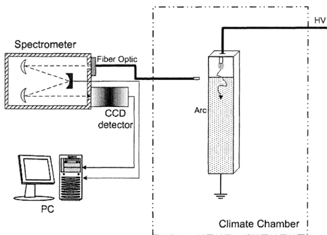
To the best of our knowledge no experimental work has ever been performed to obtain the temperatures and electron densities of arcs formed over an ice surface.This investigation is the first using a spectrometer to record the light emitted from discharge activities over an ice surface. Moreover, employing a CCD (gateable charge-coupled device) detector head on the output of the spectrometer and synchronizing the spectra with electrical measurements (current and voltage) yielded the time-resolved spectra during arc propagation from the initial stage to flashover.

Besides the originality of the methodology, this work is the first research which determined the gas and excitation temperatures, as well as the electron densities of discharges over ice based on an experimental method. It is also a pioneering work for the examination of the thermodynamic state of this type of discharge. Based on the new findings, this fundamental work will provide valuable information for the improvement of dynamic models of arc propagation.

1.4 Methodology

The spectroscopic method was chosen to achieve the afore-mentioned objectives. Light emitted from the arc is brought to the spectrometer by means of a 10-meter fiber-optic cable. Because of the practical problems associated with capturing the light emitted by the arc, a simplified test setup was chosen. First, an ice bulk was formed in a Plexiglas mould by freezing several distilled water layers in a cold chamber to achieve a flat

surface. This procedure yields a polycrystalline ice structure with semi-transparent appearance. The final layer was formed using salty water, the salt content being adjusted to reach a specified level of conductivity. Then, a 6 mm air gap was made at one end of the setup. The overall dimensions of the mould were 100 cm x 15 cm x 5 cm.

Voltage and current measurements were also performed and synchronized with recorded spectra through a data acquisition system (DAQ). The following analyses were carried out on the experimental results:

1.4.1 Rotational temperature measurements

Rotational temperatures were measured using OH (A-X) emission bands. The variation of rotational temperatures, which is similar to that of gas temperatures with discharge current, was studied. In addition, the N2+ 1st negative system was also used to measure the rotational temperatures of AC and DC applied voltages.

1.4.2 Excitation temperature measurements

Excitation temperatures of the arc column were determined using copper and oxygen lines and employing the method of relative line intensities. Deviations from LTE were taken care of using the Burton and Blade correction factor.

1.4.3 Electron density measurements

Electron densities were estimated by analyzing the Balmer line Ha profile, broadened by the Stark effect.

The above analyses were also carried out by studying the effects of voltage polarity.

1.5 Structure of the thesis

This thesis is structured as follows:

Chapter 1 presents general information about problematic, objectives, originality and general methodology.

Chapter 2 is dedicated to the review of literature.

Chapter 3 introduces the experimental equipment and the methodology. Chapter 4 presents the experimental results.

Chapter 5 discusses in detail the experimental results presented in Chapter 4. Finally, Chapter 6 concludes this work and provides recommendations for future studies.

CHAPTER 2

CHAPTER 2

LITERATURE REVIEW

2.1 Introduction

A large number of experimental investigations and theoretical studies on the subject of ice accretion on outdoor insulators have been carried out in several laboratories [13-17]. A good survey of the related literature is found in [18]. Spectroscopic plasma diagnostic methods have been used to obtain information such as temperatures of different species, electron densities, and to examine the local thermodynamic equilibrium of plasma [11, 19 and 20].

The first part of this chapter reviews spectroscopic plasma diagnostic techniques. Spectroscopic temperature measurement techniques are reviewed in the second part, including rotational and excitation temperature measurements. The next section describes the application of spectroscopic methods to measure electron densities in plasma. Studies of temperature and electron density measurements in lightning and other types of electric discharges are also reviewed. In addition, the conditions and established criteria used to verify the existence of local thermodynamic equilibrium are described.

2.2 Plasma

Plasma is often referred to as the fourth state of matter. As temperature increases, molecules become more energetic and transform in the following sequence: solid, liquid, gas and plasma. In the latter stages, molecules in the gas dissociate to form a gas of atoms and then a gas of free-moving charged particles, electrons and positive ions. This state is called the plasma state [21]. It is characterized by a mixture of electrons, ions, and neutral particles moving in random directions.

Normal state gases are electrical insulators. This is because they contain no free charged particles, only neutral molecules. If electric field of sufficient intensities is applied, they become conductive and the complex phenomena which then occur are called gas discharges.

For the various types of ionized gases, the quantities a=nl (n+n0) and degree of

ionization should be characterized. n0 is the number of neutral molecules and n is the

number of electrons. This value varies in practice between very low values of the order of 10"1 to 1. We can classify ionized gases into two groups:

Weakly ionized gases, a<10~4 Strongly ionized gases <x>10"4

When the degree of ionization is equal to unity, the density of neutral molecules is zero; the gas is then said to be completely ionized, or to constitute plasma. [22]

Plasma is electrically conductive due to the presence of free charge, and its electrical conductivities are larger than those of such metals as gold and copper. Plasma can occur naturally or be manmade. Plasma rarely occurs naturally, some phenomena such as solar corona, solar wind and lightning can however create plasma.

Because plasmas can occur over a wide range of pressures, it is customary to classify them in terms of electron densities. Most plasmas of practical significance have electron temperatures of 1 eV to 20 eV with densities in the range of 106 to 1018 cm"3.

Plasma is a region not influenced by its boundaries. As in any gas, the temperature is defined by the average kinetic energy of the particle, molecule, atom, neutral or charge. Thus, plasma will typically exhibit multiple temperatures unless sufficient collisions occur between particles to equilibrate. However, because the mass of an electron is much less than the mass of a heavy particle, many collisions are required for this to occur. [21]

Electrical discharge is one of the most common ways to create and maintain plasma. The energy from the electric field is accumulated between collisions by the electron, which subsequently transfers a portion of this energy to the heavy neutral particle, through collision. Even with a high collision frequency, the electron temperature and heavy particle temperature will generally be different.

2.3 Spectroscopic plasma diagnostics

Spectroscopic plasma diagnostics offers some important advantages that have long attracted researchers. It yields large amounts of simultaneous information about the plasma (concentration of various species of particles, temperatures) without disturbing it. In addition, spectroscopic plasma diagnostics can be applied to both transient and stationary states. [10].

Luminous emissions from arcs and plasmas often have complex spectral structures. Line spectra, particularly if time-resolved, can yield much information not

only on the nature and concentration of the species present in the discharge medium, but also on the gas and electron temperatures and electron densities. [12].

Non-thermal plasmas are characterized by a non-equilibrium distribution of energy between different species. The various temperatures describe distinct aspects of the physical state of the system:

Electron temperature is the temperature that describes, through Maxwell's Law,

the kinetic energy distribution of the free electrons.

Gas temperature describes in a similar way the kinetic energy distribution of the

gas atoms.

Excitation temperature is the temperature that describes, through Boltzmann's

Law, the relative population distribution of atoms or molecules over their energy levels. We distinguish between electronic excitation temperature, vibrational temperature, and rotational temperature.

Ionization temperature is related to the ionization equilibrium described by the

Saha-Eggert equation [23].

2.3.1 Mechanism of emission and absorption of spectra

Table 2.1 classifies the various types of spectra observed in plasma according to the particles which emit them and the degree of freedom they set into action. The atoms and ions emit a spectrum of lines from infrared to the far ultraviolet, resulting from electron excitation. At the time of electronic transition, the energy of an atom varies according to the following equation:

E -E = hv = — (2.1)

Where h is Planck's constant and the emitted radiation of frequency v is characteristic of the emitting atom for which we know the energy levels Eu (Figure 2.1).

Table 2.1. Spectra observed in plasma [10]

Particles Atom or Ion Electrons Molecules Degree of freedom Electronic excitation Ionization Translation Recombination Free-free transitions Rotation Vibration-rotation Electronic excitation Type of spectrum Line Continuum Line profiles Continuum Continuum Line Band Band systems Spectral region U.V.-visible-I.R. U.V.-visible-I.R. U.V.-visible I.R. Far infrared I.R. U.V.-visible-I.R.

The electron changing the orbit remains bound to the atom; this is called the "bound-bound" transition. The recombination of the electron and the ion corresponds to a "free-bound" transition, which gives a continuous spectrum observed in the visible and the ultraviolet.

Energy Free electrons Bound electrons Free—free f Free—bound lonization Excitation Bound-bound

Figure 2.1. Excitation levels of an atom or an ion [10]

We may also consider "free-free" transitions of free-ion electron systems for which the electrons are free before and after (Figure 2.1). Such transitions give a continuous spectrum observed in the infrared and which occurs during electron-atoms collision as well.

The diatomic molecules emit much more complex spectra. The energy diagram for CN (Figure 2.2) shows that electronic excitation occurs at energies greater than 1 eV only, whereas vibration excitation occurs at energies of some tenths of an electron volt, and rotational excitation at much lower energies still. In the far infrared, a line spectrum due to pure rotation is observed, this corresponds with transition in which only the rotational energy of the molecule changes.

In the near infrared the spectrum consists of vibration-rotation bands. With a high-resolution spectrometer, such vibration bands may be resolved into lines of rotation,

the intensities of which are related to their rotational temperatures. Finally, in the visible and ultraviolet bands, we obtain systems of electronic excitation bands [10].

Energy 6 X 10" 4 X 10 Vibrational excitation -.— " — "

7

Electronic excitation {violet system; Dissociation 3 X 10 8 cm Wavelength

Figure 2.2. Energy curves for a diatomic molecule (CN) and schematic spectrum of the violet and red systems [10].

2.3.2 Different types of emission spectra

2.3.2.1 Line spectra

In optically thin plasma, the emission coefficient corresponding to a line frequency emitted by an atom, which undergoes a transition from a higher-level u to a lower level /, is given by:

A,xNu

Nu is expressed as a function of density TV of neutral atoms. The observed line is

not infinitely narrow but always has a certain width Av;sv can be related to the spectral

emission coefficient s(v') by [10]:

sv = \s(y')dv' (2.3)

Av

2.3.2.2 Continuum spectra

In general, continuous plasma emissions are due to the superimposition of several continued spectra caused by different mechanisms:

a) Free-free radiation

This corresponds to the emission of a photon when an electron subjected to the electric field of an ion or an atom passes through a free state to another free state of lower kinetic energy.

b) Radiation due to recombination (free bound radiation)

This results from the capture of a free electron by an ion; the inverse phenomenon is photo ionization.

c) Continuum due to negative ions

This is emitted, as in the case of recombination, during the attachment of a free electron to an atom or molecule.

d) Pseudo-continuum of lines

This is due to the overlapping of neighboring lines broadened through Stark effect.

2.3.2.3 Line profiles

The lines emitted by atoms or ions are not infinitely narrow, but always show a certain profile which depends upon the environment in which the emitter is placed; in plasma, the natural broadening being always very small is negligible compared to other types of broadening: statistical Doppler effect, collisional effect, and pressure effect.

2.3.2.4 Band spectra

When the temperature of plasma does not exceed 15,000 K, its spectrum can include molecular bands, the examination of which may yield the temperatures of rotation, vibration or electronic excitation of molecules [10].

2.4 Spectroscopic temperature measurement techniques

Temperature is considered one of the most important parameters for plasma state characterization. Accurate temperature measurements lead to better understanding of the plasma processes, i.e. vaporization, dissociation, excitation and ionization [24]. In the literature dealing with plasma gas, temperature measurements are usually made using emission spectroscopy of excited plasma gas species [25]. Besides the qualitative determination of chemical composition of plasma from emission and absorption line identification, the measurement of electron and ion, or atom temperatures is the oldest application of spectroscopic methods to plasma and gaseous electrical discharge physics [26].

Non-thermal plasmas are characterized by a non-equilibrium distribution of energy between different species. Hence, the various temperatures each describe a distinct aspect of the physical state of the system [27]: the electron temperature (Te) is determined by the kinetic energy of the electrons, the rotational temperature (Trot) is relevant to all processes in which molecules, radicals, and their dissociation products are involved, and the excitation temperature (Texc) describes the population of the various energy levels [28].

2.4.1 Rotational temperature measurement

Molecular spectra can successfully give information in the temperature range of 2,000-8,000 K, where atomic spectra are not strong enough to ensure good sensitivity [29].

It can be assumed that the rotational temperature is close to the gas temperature, because rotational relaxation is fast at atmospheric pressure [8]; but the often-used assumption that Trotationai and Tvjbrationai are approximately equal to the electron temperature is not always valid in non-equilibrium plasmas [12].

The OH (A2S-X2n) transition is one of the most intense systems emitted by low-temperature air plasmas containing even a small amount (~1 %) of H2 or H2O. The rotational temperature can be derived by fitting the entire band, or more simply from the relative intensities of two groups of rotational lines corresponding to the R and P branches of the OH (A-X) (0, 0) vibrational band. These branches present distinct peaks at about 307 nm and 309 nm, respectively [8]. This technique provides a sensitive thermometer, because the relative intensity of the two peaks varies rapidly with the

rotational temperature. Another advantage of the technique is that it does not require absolute or relative intensity calibration because the response of usual detection systems is nearly constant over the small spectral range of interest [8].

Generally the value of the rotational temperature of the OH radicals is close to the gas temperature. The OH band diagnostic applies to a wide temperature range and even to non-equilibrium plasmas [30].

Bands of NO, OH, and O2 dominate the spectrum at temperatures below ~5,000K. The second positive system of N2 (C-B), the first negative system of N2+ (B-X), and atomic lines of O and N appear at higher temperatures [8].

For low-temperature plasmas in humid air, the emission spectrum of the OH (A-X) transition around 300 nm provides a convenient way to measure the rotational temperature. At higher temperatures, or in the presence of an electric field, the OH transition is overlapped by strong emissions from N2 (C-B) (second positive system). In this case, the rotational temperature can be measured from N2 (C-B) rotational lines [8].

The rotational lines of the N2+ first negative system (B2S+-X2S+), particularly those of the (0-0) band, have often been used to determine rotational and vibrational temperatures in plasma [31, 32].

The group of rotational lines of the N2+ first negative system in the region of 380 nm to 392 nm is well isolated from lines of other transitions. Their lines are sensitive function of rotational temperature, but they appear at higher temperatures [8].

The intensity Inm of a spectral line corresponds to a transition between two levels

(n—*m), derived from [33]:

^ e p ( )^ (2.4)

Where k is the Boltzmann constant, Knm is a constant for a given transition

in-^m), Z (T), the partition function of the particle, and Em the energy of the state n.

When Inm is known for a given temperature Tref (/„„, ref is used as reference), one

can read [33]:

In their work, Dieke and Crosswhite [34] provided the wavelengths of the different branches, the energy of the upper level of each transition, and the normalized intensity Inm-ref of each line of the rotational band OH (A-X) for a reference temperature of Tref =3000K. The term Z (3000)/Z (T) is the same for all rotational lines issued to the upper vibrational level n. From that viewpoint, this term is normalized to one in the evaluation of Equation (2.5) [35]. SPECAIR software [36] can be used to calculate the theoretical spectra of each rotational temperature, considering the slit function of the spectroscopic system.

2.4.2 Excitation temperature measurement

The spectral lines are due to the quantization of energy levels in atoms, ions, molecules or particles, resulting from transitions from one energy level to another, accompanied by the release or absorption of photons. Rest wavelengths of the lines can be accurately derived from quantum mechanical calculations or laboratory measurements. From the intensities of lines of the same atom, ion or molecule, and detailed calculations of the transition probabilities, it is possible to determine the density and temperature of the region in which it arises [37].

In many cases, it is necessary to distinguish between kinetic temperatures of electrons, ions, and atoms, say, Te, T2 and Ta. These temperatures may differ from each other even if the individual velocity distributions are close to Maxwellians, because electron-electron energy transfer rates are much larger than electron-ion collision rates, as are ion-ion rates [37].

Most of the spectroscopic temperature measurements primarily yield Te. They are based on:

• Relative line intensities either of the same atom or ion of neighbouring ionization stages or of successive isoelectronic ions;

• Relative continuum intensities, on ratios of line and continuum intensities;

• Relative and absolute intensities from optically thick plasmas; • Time histories of emission from transient plasmas [37].

Several techniques are based on this concept. In the Boltzmann method [38], the absolute intensity of a spectral line involved in the transition from an upper level q to a lower level p is:

d g

U

= A n

Where d is the depth of emission source, Aqp is the transition probability of q to p,

n is the population of the i'h excited state, gq is the known statistical weight or degeneracy

of the excited state, Z is the partition function, eq is the excitation energy, k is the

Boltzmann constant, T is the absolute temperature, h is the Planck constant, and vqp is the

frequency of the spectral line emitted in the transition from q to p. Taking the logarithm of both sides of this rearranged equation, we have:

(2-7)

If we plot the left hand side of this equation versus the excitation energy (e9), a linear relationship with a slope of (-1/KT) is obtained, often referred to as the Boltzmann plot [37].

In the modified Boltzmann method [37], the temperature can be derived from the s I

slope of the plot between log( q qp ) and sq.

Another variation of the Boltzmann method uses the intensity ratio of two lines [37]. If the lines are labelled a, b, respectively, and subscripts p and q are omitted for the sake of convenience, we obtain:

T = TTT—a*l-<e°-e>>/krJ ( 2-8 ) h (A)

Rearranging this equation, we obtain:

T = 5040(rflrt)

l ( ( 4 ) J(gA)h)- l o g a IXb)~ log(/a IIh)

• F is the excitation potential (eV)

A is the (relative) transmission probability

• g is the statistical weight • X is the wavelength • / is the (relative) intensity

In this method, both lines should belong to the spectrum emitted by the neutral atom or the ion of an element. Furthermore, the difference between the excitation potentials Va and Vb should be sufficiently large.

The measurement of arc properties by atomic emission spectroscopy relies on the existence of a local thermodynamic equilibrium (LTE). Another method that may be used down to ambient temperatures is laser-scattering temperature measurement, essentially independent of LTE [39].

Another variation of the Boltzmann method considers two different spectral lines, the absolute temperature being determined from the relative intensities of these two lines with known relative transition probability, as follows [37]:

T= {E«-E")lk (2.10)

U,

s,. L ÏJ

• Em is the excitation potential of the mth level (eV)

• k is the Boltzmann constant

• Imp is the intensity of transition from level m to level/»

• gp is the statistical weight of theplh level

• / i s the absorption oscillator strength for a particular transition • X is the wavelength (nm)

The criteria for selecting lines in the emission spectrum can be determined by performing an error analysis on (2.10):

AT \n\(ï + AR/R)/(\ + AF/F)] (2 ID

T ~ (£,„-£„)/

1/R is the intensity ratio Inr IImp

The range of error can thus be minimized by choosing a large Em-En. It could be

also minimized by choosing strong lines of approximately equal intensity [37].

When the local thermodynamic equilibrium deviates, the non-equilibrium parameter b (defined as the ratio of the actual to calculated LTE level populations) may be used [40]. Using this method proposed by Burton and Blades [40], the actual populations can be calculated, allowing theoretical Boltzmann plots to be constructed. Hence, the intensity of a spectral line resulting from transition from level mXo n is:

A

4 zintCO

Where Amn is the transition probability, kmn is the wavelength between the upper

level m and lower level n, gm is the statistical weight, and Em is the energy of the upper

level; n, is the total number density of chemical species /, zinl(Texc) is the internal partition

function calculated at temperature Texc, and b™lom is a non-equilibrium parameter that can

be evaluated for the considered atom as [40] :

b lalom

where Ex is the ionization energy (eV) and ne is the electron density expressed in

cm"3.

2.5 Spectroscopic density measurement techniques

Depending on various plasma conditions, such as size, composition, densities and temperatures, electron densities can be measured using a number of techniques. Langmuir probes provided the first means to infer local values of electron density, mostly

at relatively low densities. Thomas scattering of laser light has become a method of choice for localized electron density measurements over a range of about 10n to 10 ! cm"3 [26].

The purely spectroscopic density determinations are based on the interpretation of measurement of at least one of the following quantities: spectral line widths or profiles, absolute continuum intensities, absolute line intensities, or relative line intensities. In general, this interpretation depends on some knowledge of the temperature. Generally, an iterative procedure also using the methods of temperature determination is called for. In practice, this iterative method is replaced by comparing measured and synthetic spectra, the latter being calculated for sets of assumed plasma conditions until a satisfactory fit is obtained [26].

Densities from spectral line widths and profiles

Under favorable circumstances the widths, shifts and profiles of suitable spectral lines are very insensitive to both electron and ion temperatures [26].

One of the common electron density measurement methods consists in making use of the Stark effect. This effect involves the interaction between radiating atoms or ions and electrons or ions [12], and therefore depends on charged particle densities. In fact, the effect depends primarily on the densities of charged particles and is only a weak function of temperature [41]. Stark widths and profiles of many spectral lines are found in Griem [42].

The most important experimental considerations for choosing spectral lines for plasma density measurements are their strengths and separation from neighboring lines; and also the wavelength range, i.e., the relative ease of obtaining sufficient resolution and

signal. On the theoretical side, it is important that broadening mechanisms other than the Stark effect are ruled out, or at least accounted for. Doppler broadening can be calculated if the atom or ion kinetic temperatures are known. Instrumental broadening should be measured separately. Both effects are best accounted for by including them in any simulated spectra. If this is not possible, they should be allowed for in error estimates [26].

The principal advantages of using synthetic spectra for comparisons with measured data before inferring electron densities are the possibility of fitting entire profiles, rather than only comparing measured and calculated line widths, and the ease of accounting for variations of plasma conditions along the line of sight [26]. It is preferable to use optically thin lines with high intensities that are highly sensitive to Stark effects. A good example in this category is the Hp line of hydrogen. At temperatures near 1 eV, can be applied to electron densities from 1014 to 1017 cm"3. At 10 eV, only densities above 1015 cm"3 can be determined reliably due to grater Doppler broadening. Above Ne = 1017 cm"3, it is preferable to use the less sensitive Ha line, because the Hp line becomes too broad for a clean separation from the underlying continuum and from the Hy line [26].

Since the Stark profiles are only weak functions of temperature, measured values can be used to determine electron densities in situations where the temperature is only approximately known, or even when the existence of a unique temperature is questionable e.g. when LTE is not achieved [43].

The Lorentzian function is used to describe Stark broadening and is expressed as follows:

S(X;X0,y) = -71

y/2

(2.14)

• S (X; ko, y) is the light intensity • Xo is the central wavelength of the line

• y is the scale parameter which specifies the FWHM (Full Width at Half Maximum).

Electron densities can be obtained directly from the profile widths [26] or by fitting the data to theoretical line profiles [44]. Because of theoretical developments, the half-width measurement of Stark-broadened lines now ranks as one of the most accurate and convenient methods for determining electron densities [45]. In principle, one must match the measured line profiles and the calculated Stark profiles properly within a range of electron densities. The correct density corresponds to the best-fit Stark profile [46]. However, a more reliable and still simple method is the standard procedure for deriving electron densities from measured line widths [46, 47].

In laboratory-created plasma, the Balmer-a (Ha) line of hydrogen, due to transitions between principal quantum number n=3 and 2 levels, often is a prominent line [48]. The line shape strongly depends on the density of charged particles surrounding the emitter. Due to the decomposition of water vapor during discharge activities on the ice surface, hydrogen is present in the arc column, and the Ha line of the Balmer series is considerably Stark-broadened so that electron density may be determined by comparing the measured profiles with theoretical profiles [26].

2.6 Arc discharge temperature and electron density

measurement

There are a lot of different methods for studying electrical discharge phenomena. They can be divided into two main categories: optical and electrical measurements. In this study only the "Spectroscopic analysis" method is described.

The pioneering works of Uman [19] and Orville [11] are good references for measuring the temperatures and electron densities of lightning using the spectroscopic method. Uman and Orville [19] measured the electron (ion) densities in three different lightning strokes by observing the Stark-broadening of the Ha lines in lightning spectra. They concluded that the electron density in the stroke when the maximum integrated intensity from Ha was being recorded was between lxlO17 and 5xlO17 cm"3. Orville [11] employed the ratio of intensities of emission lines to calculate the temperature of a ~10 m section of return-stroke channel. The peak temperatures were in the 28,000-31,000 K range. He used the Stark-broadened half-width of the Ha line and calculated an electron density in the order of 8x1017 cm"3 in the first 5 (asec, decreasing to l-1.5xlO17 cm"3 at 25 ]xs. They also performed the same study on long air gaps [49], [54].

Les Renardières Group [50], [51] applied spectroscopic analysis to obtain time-resolved information on the physical process occurring at different stages of breakdown of long gaps using two spectrometers and a streak camera. They observed the different spectral distributions between leader coronas and leader channel phenomena. The leader coronas were predominantly in the ultraviolet region, about 300 nm, while the leader channel was in the red, between 500 nm and 700 nm [50].

They observed different lines of neutral and ionized nitrogen and oxygen and also the atomic hydrogen lines Ha and Hp in their recorded spectra of leader channels [52]. They derived gas and electron temperatures and ionization degrees in the leader channels and compared their results with Orville [49] and Vassy [53]. Figure 2.3 shows their results [52].

accroissement transitoire de pression T(1O °K) transition pressure increase

40 35 30 25 20 15 10 S

choc de faible Intensité / onde de choc ' 'équilibre de pression / ^ décroissance de pressio

weak shock shock wave .pressure equilibrium , \ , pressure decrease

, \ 10" non L TE electronic excitation ETL excitation thermique LTE thermal excitation thermalization phase 12 18 24 tips) LTE equilibrium with T

Figure 2.3. Gas and electron temperature and ionization degree in the leader channel, comparison of Les Renardières Group [52] results with Orville [49] and Vassy [53]

Uman et al. [54] investigated a four-meter spark in air, using streak photography and spectroscopy. They observed that primary radiating species in the leader is singly ionized nitrogen (N II) and estimated the leader temperature to be in the order of 20,000K.

Staaek et al. [55] experimented with DC glow discharges in atmospheric pressure helium, argon, hydrogen, nitrogen and air. They measured the rotational temperatures using the Avib +2 transitions of the N2 2nd positive system for the various discharge gases relative to discharge current. The gas temperatures for a 3.5 mA normal glow discharge

were around 420 K , 680 K, 750 K, 890 K and 1,320 K in helium, argon, hydrogen, nitrogen and air, respectively. They also used atomic transitions to determine the electronic excitation temperatures for different upper-state energies on Boltzmann plots which indicated a non-thermal discharge [56].

Shinobu et al. [57] preformed a spectroscopic study of 150 W plasma in water. The Balmer atomic hydrogen lines (Ha and Hp), OH (A-X) (0, 0) band at 309 nm, O (777 nm) and O (845 nm) were detected as strong emissions. In addition to HY, peaks of O I and O II were also detected as weak emissions. The Na line (589 nm) also appeared as an impurity in the spectra. They measured electron temperatures from the ratio of the emission intensities of Ha and Hp and rotational temperatures of OH radicals was obtained from OH A2£-X2n (0, 0) band emissions [57].

Nieto-Salazar et al. [58] carried out spectroscopic studies of positive streamers in water. The light emitted by streamers showed the UV OH band, atomic lines of OI, Ha and a strong continuum from 350 nm to 500 nm. Rotational temperatures were calculated from OH bands to be in the range of 3,000 K to 4,000 K, and the electron densities were measured from Stark broadenings of Ha and OI (777nm) to be in the order of 1017 cm"3.

Gas temperatures, electron densities and electron temperatures of excited plasma were measured by optical emission spectroscopy by Xi-Ming Zhu et al. [59]. The gas temperatures were obtained from the rotational temperatures of the hydroxyl molecule (A 22+, v = 0) and the electron densities were measured by the Stark broadening of the hydrogen Balmer p line. The electron temperatures were estimated based on the measured excitation temperatures of Argon 4p and 5p levels [59].

2.7 Thermodynamic study of plasma

The condition of the arc plasma can be regarded as a state of thermal equilibrium when all definitions of temperature give the same numerical values. In non-equilibrium sources, different definitions will, in general, lead to different values of the parameter.

The various temperatures each describe a distinct aspect of the physical state of the system [27] :

Electron temperatures, which are determined by the kinetic energy of the electrons; gas temperatures, which are defined by the kinetic energy of the neutral atoms; excitation temperatures, which describe the population of the various energy levels; and ionization temperatures, which govern the ionization equilibrium.

2.7.1 Thermal equilibrium in the arc

For gases to be in complete thermal equilibrium, the various gas components, i.e. neutral particles, charge carries, and photons, must be in equilibrium mutually and with respect to the surroundings. Complete thermal equilibrium (C.T.E) prevails in an enclosure whose walls and interior have a uniform temperature with respect to radiation and internal energy.

A gaseous system in C.T.E is characterized by the following conditions:

1. The velocity distributions of all kinds of free particles (molecules, atoms, ions and electrons) at all energy levels satisfy Maxwell's law.

2. For each separate kind of particle the relative population of energy levels conforms to Boltzmann's distribution law.

3. Ionization of atoms, molecules and particles is described with Saha's equation.

4. Radiation density is consistent with Plank's Law [16].

2.7.1.1 Maxwell's Law

In thermal equilibrium conditions, the speeds of particles are distributed according to the Maxwell's function.

f(v)dv = (-^—y/2(e 2KT )4xv2dv (2.15)

2nKT

Where v is the frequency of the photon emitted in the transition, T is temperature, and/(v) is the fraction with speeds between(v, v + dv) [60].

2.7.1.2 Plank's Law

The black body is an ideal body of uniform temperature T (K) that perfectly absorbs all incidental radiation, and emits isotropically unpolarized thermal radiation according to Planck's Law. It is customary to indicate with B\ (T):

In wavelength units, the emission is:

Bx (T) = ^ ^ erg.cm-2s-xcm'x s (2.16)

Where BÀ (T) is the specific intensity energy per unit area per unit time per unit

bandwidth, h is Plank's constant, h = 6.57 x 10~27 erg.s"1, k is Boltzmann's constant, X

25000 K 20000 K

0 200 400 600 800 1000 1200 nm

À

Figure 2.4. Plank's distribution [61]

Equilibrium between light quanta and material particles in an arc column is not expected to be reached owing to the absence of walls with the same temperature as the arc gas, and hence the radiation density is not expected in general to satisfy Planck's Law. But with increasing concentrations of emitting and absorbing particles the intensity in the center of the spectral line asymptotically approaches the intensity of blackbody radiation at the same temperature and wavelength. Under such conditions, the radiation density distribution may thus be assumed, to a good approximation, to be consistent with the upper limit of Planck's Law [61]. Furthermore, the energy loss from the arc by radiation amounts to only a few percent of the total energy supply. For this reason a state of partial thermal equilibrium can exist [27].

2.7.1.3 Saha's equation

The basic concept of thermal ionization introduced by Saha is the application of the mass action law to ionization equilibria. For each component (labeled i) of a composite gas we can consider on equilibrium of the form:

neutral atom <t=> ion + electron

The equilibrium constant Kn = iJ -e can be calculated as a function of

temperature. The resulting equation Knj = Snj(T) is known as Saha's relationship, where

riy and naj are the densities and concentrations of the ions and neutral atoms of the

component labeled/, and ne is the electron density.

The dependence of the ionization constant Snj on temperature is expressed by

Saha's equation:

P

^

^

( 2

,

7 )

naj

Where m is the electronic mass, k, the Boltzmann constant, h, the Plank constant, Z, the partition function, and s, the ionization energy. The factor 2 that immediately precedes the ratio of partition function is the statistical weight of a free electron [27].

2.7.1.4 Boltzmann's Law

If a gaseous body in an enclosure is in thermal equilibrium with the walls, the population of energy levels for each separate kind of particle follows as Boltzmann distribution, namely:

( )

"o So

Where nq is the density or concentration of particles in the excited state q, n0 is

the density of ground state atoms, g and g0 are the statistical weights of the

corresponding levels, sq is the excitation energy of the state q, k is the Boltzmann

constant, and T, the absolute temperature.

The statistical weight of a particular state is the probability of populating a state under identical conditions. Under those conditions we have "detailed balancing", i.e. in equilibrium the total number of particles leaving a certain quantum state per second equals the number arriving in that state per second, and the number leaving by a particular path equals the number arriving by the reverse path [27].

2.7.1.5 Partition function

To drive the equation we write, instead of Boltzmann's equation:

n0 : nx : n2 : ...nj = g0 : gx exp^^j / kT) : g2 e x p ^ IkT) : ...gj Qxp(-£j I kT) (2.19)

Where the energy of levels 1, 2... j is taken from ground level zero. Now, since: m=j

JX=w (2.20)

m=0 We have: \ = o q — x-v -q- - , ( 2 2 1 ) n '-o

j

If we put Z = ^ gm exp(-£m / kT), which is called the partition function (or the

o

sum over states) of the particular atom, the summation will include all possible energy levels of the relevant particle [27].

The importance of the partition function Z is that in Maxwell-Boltzmann and classical statistics, all the thermodynamic properties of a system can be expressed in terms of Z and its partial derivatives [62].

To distinguish the quantities n and Z of neutral atoms and singly charged ions, the g of ions is distinguished from that of atoms. Accordingly, for atoms we write:

l ^ q (2.22)

A similar equation holds for ions. The practical form of expression is:

q (2.23)

Where Vq is the excitation potential expressed in electron volts.

The above equation is often conveniently employed in its logarithmic form, as in [16].

l og »«, = log na + log gq — Vq - log Za (2.24)

2.8 Thermodynamic equilibrium

When an arbitrary system is isolated and left alone, its properties will in general change with time. If initially there are temperature differences between parts of the

system, after a sufficiently long time the temperature even out at all points, and then the system is in thermal equilibrium.

If there are variations in pressure or elastic stresses within the system, parts of the system may move, or expand, or contact. Eventually this motions, expansions, or contractions will cease, and then the system is in what is called mechanical equilibrium.

Finally, suppose the system contains substances that can react chemically. After a sufficiently long time has elapsed, all possible chemical reactions will have taken place, and the system is then said to be in chemical equilibrium.

A system, which is in thermal, mechanical, and chemical equilibrium, is said to be in thermodynamic equilibrium [62].

2.8.1 Thermodynamic properties

2.8.1.1 Mass density

Considering a gas at thermodynamic equilibrium consisting of different species /, with mass m\ and density Nt, the mass density will be [60] :

W, (2.25)

2.8.1.2 Enthalpy

In thermodynamics and molecular chemistry, the enthalpy, or heat content, (denoted as H or AH) is a quotient, or description, of the thermodynamic potential of a

system, which can be used to calculate the useful work obtainable from a closed thermodynamic system under constant pressure. By definition:

H=U+pV (2.26) Where U is the internal energy, p is the pressure and V is the volume [63].

2.8.1.3 Heat Capacity at constant pressure

The variation of enthalpy with temperature at constant pressure is also an extensive property called Heat Capacity at constant pressure and denoted by Cp [63]:

2.8.2 Composition and thermodynamic properties of

two-temperature plasma

Up to now it has been assumed that ions, neutral particles, and electrons have Maxwellian distributions, and that collisions between these particles are numerous enough to allow equalization of energies between the heavy and light particles. Such a hypothesis leads to a unique temperature (defined as the mean kinetic energy) for both heavy and light particles.

However, if the pressure is lowered or the electric field increased (for example near the electrodes of arcs in atmospheric pressure) and where there are large gradients (near cold walls or when a cold gas is injected into the plasma), equilibrium will no longer exist. When the energy gained by the electrons between two collisions is no longer

negligible compared with the thermal energy kTe, the electron temperature Te differs from that of the heavy species Th [64].

2.8.3 Local Thermodynamic Equilibrium

When a gas is in thermodynamic equilibrium, it is possible to calculate the particle densities of all the species in terms of the thermodynamic state of the gas.

Partially ionized gases are rarely in complete thermodynamic equilibrium, but they may frequently be in a state of approximate Local Thermodynamic Equilibrium, or LTE. A gas is said to be in LTE when the matter particles are in equilibrium with each other, but when the photons are not in equilibrium with the matter. In most situations, a partially ionized gas is transparent in many frequency intervals, and some radiation therefore escapes from the gas, thus violating a condition necessary for complete thermodynamic equilibrium. For the matter to be in LTE, the collisional rates that populate and depopulate the various energy levels of the matter must exceed the corresponding radiative rates. For a gas in LTE, the Boltzmann and Saha relations can be used even though complete thermodynamic equilibrium does not prevail.

For collision-dominated gases the Boltzmann and Saha relations are often applicable even when other kinds of departures from complete thermo-dynamic equilibrium occur.

It is often possible for the electrons to have a temperature Te that differs from the heavy particle temperature Th: Both types of particles may still have Maxwellian velocity distributions, but at different temperatures. When it is primarily collisions with electrons which produce the transitions that determine the population of some energy level or the