Do Peers Affect Student Achievement? Evidence from Canada Using Group Size Variation

Texte intégral

(1)2010s-08. Do Peers Affect Student Achievement? Evidence from Canada Using Group Size Variation Vincent Boucher, Yann Bramoullé, Habiba Djebbari, Bernard Fortin. Série Scientifique Scientific Series. Montréal Février 2010. © 2010 Vincent Boucher, Yann Bramoullé, Habiba Djebbari, Bernard Fortin. Tous droits réservés. All rights reserved. Reproduction partielle permise avec citation du document source, incluant la notice ©. Short sections may be quoted without explicit permission, if full credit, including © notice, is given to the source..

(2) CIRANO Le CIRANO est un organisme sans but lucratif constitué en vertu de la Loi des compagnies du Québec. Le financement de son infrastructure et de ses activités de recherche provient des cotisations de ses organisations-membres, d’une subvention d’infrastructure du Ministère du Développement économique et régional et de la Recherche, de même que des subventions et mandats obtenus par ses équipes de recherche. CIRANO is a private non-profit organization incorporated under the Québec Companies Act. Its infrastructure and research activities are funded through fees paid by member organizations, an infrastructure grant from the Ministère du Développement économique et régional et de la Recherche, and grants and research mandates obtained by its research teams. Les partenaires du CIRANO Partenaire majeur Ministère du Développement économique, de l’Innovation et de l’Exportation Partenaires corporatifs Banque de développement du Canada Banque du Canada Banque Laurentienne du Canada Banque Nationale du Canada Banque Royale du Canada Banque Scotia Bell Canada BMO Groupe financier Caisse de dépôt et placement du Québec DMR Fédération des caisses Desjardins du Québec Gaz Métro Hydro-Québec Industrie Canada Investissements PSP Ministère des Finances du Québec Power Corporation du Canada Raymond Chabot Grant Thornton Rio Tinto State Street Global Advisors Transat A.T. Ville de Montréal Partenaires universitaires École Polytechnique de Montréal HEC Montréal McGill University Université Concordia Université de Montréal Université de Sherbrooke Université du Québec Université du Québec à Montréal Université Laval Le CIRANO collabore avec de nombreux centres et chaires de recherche universitaires dont on peut consulter la liste sur son site web. Les cahiers de la série scientifique (CS) visent à rendre accessibles des résultats de recherche effectuée au CIRANO afin de susciter échanges et commentaires. Ces cahiers sont écrits dans le style des publications scientifiques. Les idées et les opinions émises sont sous l’unique responsabilité des auteurs et ne représentent pas nécessairement les positions du CIRANO ou de ses partenaires. This paper presents research carried out at CIRANO and aims at encouraging discussion and comment. The observations and viewpoints expressed are the sole responsibility of the authors. They do not necessarily represent positions of CIRANO or its partners.. ISSN 1198-8177. Partenaire financier.

(3) Do Peers Affect Student Achievement? Evidence from Canada Using Group Size Variation* **. Vincent Boucher †, Yann Bramoullé ‡, Habiba Djebbari §, Bernard Fortin Résumé / Abstract. Nous présentons une première application empirique d’une nouvelle approche développée par Lee (2007) pour estimer les effets de pairs dans un modèle linéaire-en-moyenne. Cette méthode permet de tenir compte des variables non-observées au niveau du groupe et de solutionner le problème de réflexion. Nous estimons les effets de pairs sur la performance scolaire (mesurée par les résultats aux épreuves du ministère de l’Éducation, du Loisir et du Sport) en Mathématiques, en Science, en Français et en Histoire dans les écoles secondaires du Québec. À cette fin, nous utilisons des méthodes de maximum de vraisemblance et de variables instrumentales. Nos résultats corroborent la présence d’effets de pairs. L’effet de pair endogène est positif, lorsqu’il est significatif. En particulier, une hausse d’un point dans la note moyenne de ses pairs accroît la note de l’élève de 0,5 en Français, de 0,65 en Histoire et 0,83 en Math (514). En outre, certains effets contextuels ont de l’importance. À partir de simulations Monte Carlo, nous trouvons qu’une grande variabilité dans la taille des groupes peut réduire les problèmes d’identification faible. Mots clés : effets de pairs, performance scolaire, problème de réflexion. We provide the first empirical application of a new approach proposed by Lee (2007) to estimate peer effects in a linear-in-means model. This approach allows to control for group-level unobservables and to solve the reflection problem. We investigate peer effects in student achievement in Mathematics, Science, French and History in Quebec secondary schools. We estimate the model using maximum likelihood and instrumental variables methods. We find evidence of peer effects. The endogenous peer effect is positive, when significant, and some contextual peer effects matter. Using calibrated Monte Carlo simulations, we find that high dispersion in group sizes helps with potential issues of weak identification. Keywords: peer effects, student achievement, reflection problem. Codes JEL : C31, I20, Z13. *. An early version of this article was presented at the CIRANO-CIREQ Conference on the Econometrics of interactions (October 2009). Our thanks to conference participants, in particular to Lung-fei Lee for helpful comments. We wish to thank the Quebec Ministry of Education, Recreation and Sports (MERS) for providing the data, in particular Raymond Ouellette and Jeannette Ratté for their assistance in obtaining and interpreting the data used in this study. The views expressed is this paper are solely our own and do not necessarily reflect the opinions of the MERS. We thank Steeve Marchand for helpful research assistance. Support for this work has been provided by the Canada Chair of Research in Economics of Social Policies and Human Resources, le Fonds Québécois de Recherche sur la Société et la Culture and le Centre Interuniversitaire sur le Risque, les Politiques Économiques et l’Emploi. † Université de Montréal. ‡ CIRPÉE and Department of Economics, Université Laval § CIRPÉE, IZA and Department of Economics, Université Laval ** Corresponding author: CIRANO, CIRPÉE, and Department of Economics, Université Laval, Department of Economics, Université Laval, Quebec, Canada. Email: bernard.fortin@ecn.ulaval.ca.

(4) 1. Introduction. Evaluating peer effects in academic achievement is important for parents, teachers and schools. These effects also play a prominent role in policy debates concerning ability grouping, racial integration and school vouchers. However, despite a growing literature on the subject (e.g., Sacerdote 2001, Hanushek et al. 2003, Angrist and Lang 2004, Stinebrickner, R. and Stinebrickner 2006, Ammermueller and Pischke 2009), the evidence regarding the magnitude of peer effects on student achievement is mixed. This lack of consensus partly reflects various econometric issues that any empirical study on peer effects must address. Identifying and estimating peer effects raises at least three challenges. First, the relevant peer groups must be determined. Who interacts with whom? Second, peer effects must be identified from confounding factors. Especially, spurious correlation between students’ outcomes may arise from self-selection into groups and from common unobserved shocks. Third, identifying the precise type of peer effect at work may be hard. The reflection problem may prevent separating contextual effects, i.e., the influence of peers’ characteristics, from endogenous effects, i.e., the influence of peers’ outcomes, see Manski (1993). Researchers have used various approaches to solve these three issues; we discuss the methods and results of previous studies in more detail in the next section. As will be clear, however, there is no simple methodological answer to these three challenges. In this paper, we provide, to our knowledge, the first application of a novel approach developed by Lee (2007) for identifying and estimating peer effects. This approach is promising, as it allows to solve the problem of correlated effects and the reflection problem with standard data and without imposing ad hoc exclusion restrictions. The method does rely on structural assumptions, however, which makes its confrontation to real data particularly important. We have collected for this analysis original administrative data on test scores at the end of secondary school in the Canadian province of Quebec. We investigate the presence of peer effects in student achievement in mathematics, science, french, and history by applying Lee (2007)’s approach. In the process, we also advance our understanding of the method’s properties. Our econometric model relies on two key assumptions. First, individuals interact in groups that are known by the modeler. This means that the population of students is partitioned in groups (e.g., classes, grade levels) and that students are affected by all others in their groups but by none outside of it. This assumption is typical in studies of academic achievement but clearly arises from data constraints.1 Second, individual outcome is determined by a linear-in-means model with group fixed effects. Thus, the test score of a student is affected 1. Recent studies have looked at peer effects within finer social subdivisions such as networks of friendships among students, see Lin (2008) and Calvó-Armengol et al. (2009) for applications, and Bramoullé et al. (2009) and Lee et al. (2009) for theoretical analyses.. 1.

(5) by his characteristics and by the average test score and characteristics in his peer group. In addition, it may be affected by any kind of correlated group-level unobservable. Lee (2007) shows that peer effects are fully identified in such a framework. The intuition for this result is the following. To address the problem of correlated effects, the group-level fixed effects must first be differentiated out. This removes any factor common to everyone in the group. In this model, however, a student is not assumed to be one of his own peer. This creates individual variations in average peer attributes, which are mechanically greater in smaller groups.2 These variations survive the elimination of common unobservables. They lead to a non-linear impact of group sizes on reduced-form coefficients which can be used to recover the structural parameters.3,4 More precisely, contextual and endogenous peer effects are identified when there are at least three groups of different sizes, see Davezies et al. (2009). When identified, the model can then be estimated through methods adapted from spatial econometrics, e.g. Cliff and Ord (1981). We use administrative data on academic achievement for a large sample of secondary schools in the province of Quebec obtained from the Ministry of Education, Recreation and Sports (MERS). Our dependent variables are individual scores on four standardized tests taken in June 2005 (Math, Sciences, French and History) by fourth and fifth grade secondary school students. All 4th and 5th grade students in the province must pass these tests to graduate.5 One advantage of these data is that all candidates in the province take the same exams, no matter their school and location. This feature effectively allows us to consider test scores as draws of a common underlying distribution. Another advantage is that our sample is representative and quite large. We have the scores of all students for a 75% random sample of Quebec schools which, over the four subjects, yields 194,553 test scores for 116,534 students. In terms of interaction patterns, the structure of the data leads us to make the following natural assumption. We assume that the peer group of a student contains all other students in the same school qualified to take the same test in June 2005. In practice, a small number of students postpone test-taking to August 2005. We extend Lee’s methodology in the empirical modelling to address this issue. However, since the difference between observed group sizes and actual group sizes is small, the correction has little effect on the 2. In contrast, these variations are absent in the model studied by Manski (1993). Manski studies a linear-in-expectations model which, in terms of identification, has the same properties as a linear-in-means model where the individual is included in his peer group. In this case, group fixed effects wash out both types of peer effects and identification fails to hold. 3 This result is to be distinguished from the idea that the group size is a factor in a school’s production function (e.g., Angrist and Lavy 1999, Hoxby 2000b, Krueger 2003). In our model the effects of group sizes which are separable from the peer effects are controlled for by fixed effects in the structural model. 4 This method also differs from the variance contrast approach developed by Graham (2008), which builds on Glaeser et al. (1996). The basic idea in this approach is that peer effects will induce intragroup dependencies in behavior that introduce variance restrictions on the error terms. These restrictions allow to identify the composite (endogenous + contextual) social interaction effects under the assumption that the variance matrix parameters are independent of the reference group size. 5 These tests are taken once all courses in a subject matter are completed. Success to these tests only partly determine secondary school graduation, which also depends on performance in year-long evaluations.. 2.

(6) results. Following Lee (2007), we estimate the model in two ways: through generalized two-stage least squares (G2SLS)6 and, under stronger parametric conditions, through conditional maximum likelihood (CML). Overall, we find that the CML method yields relatively precise estimates of peer effects.7 In contrast, estimates from instrumental variables methods are quite imprecise with our data.8 Based on CML estimates, the endogenous peer effect is positive, significant and quite high in Math (0.82) and History (0.65) but not significantly different from zero in French (0.33) and Science (−0.23).9 These results are on the high side, but still within the spectrum, of estimates obtained in other studies. We also find evidence that contextual peer effects matter. For instance, interacting with older students usually has a negative effect on own test score independent of the impact of others’ scores. While endogenous peer effects may capture direct emulation and imitation, contextual peer effects may reflect more indirect social interactions. In any case, this approach allows us to test typical restrictions used in the literature to get around the reflection problem. We often reject these restrictions in favor of the full, unrestricted model. This shows, a posteriori, the interest of disentangling the different types of peer effects. One potentially important limitation of the method, however, is that it may not perform well when group sizes are large, see Lee (2007). More precisely, convergence in distribution of the peer effect estimates may occur at low rates when the number of groups is not much larger than average group size. Ratio between the two lies between 2.36 and 7.23 in our sample, so weak identification may be an issue. On the other hand, there is also much variance in group sizes in our samples. We suspect that this dispersion helps identification. We study this issue systematically through Monte-Carlo simulations. We find that indeed increasing group size variance has a strong positive impact on the precision of estimates. In addition, simulations calibrated on our data indicate that these small-sample problems are likely not an issue for our main empirical results. The remainder of the paper is organized as follows. We discuss past research in section 2 and present our econometric model and the estimation methods in section 3. We describe our dataset in section 4. We present our empirical results in section 5 and run Monte Carlo experiments in section 6. We conclude in section 7. 6. The instruments are directly derived from the structural model (Kelejian and Prucha 1998, Lee 2003, Lee 2007), see section 3.2.2 for details. 7 The effect of individual characteristics, such as gender, age, and socioeconomic background, on test scores are precisely estimated by either method, and these estimates generally conform to expectations. 8 The higher precision of CML estimates is consistent with results in Lee (2007) showing that CML estimators are asymptotically more efficient than IV estimators. 9 For the French test, we also look at an alternative formulation under which the endogenous effect is equal to 0.51 and is significant.. 3.

(7) 2. Previous research. In this section, we give a brief overview of the recent literature on student achievement and peer effects, and we explain how our study complements and enhances current knowledge on peer interactions in academic outcomes. As discussed above, measuring peer effects is complex as it raises three basic interrelated problems: the determination of reference groups, the problem of correlated effects and the reflection problem. The choice of reference groups is often severely constrained by the availability of data. In particular, there are still few databases providing information on the students’ social networks; the Add Health dataset is an exception, see e.g. Lin (2008) and Calvo-Armengol et al. (2009).10 For this reason, many studies focus on the grade-within-school level (e.g., Hoxby 2000a, Hanushek et al. 2003, Angrist and Lang 2004).11 Other studies analyze peer effects at the classroom level (e.g., Kang 2007, Burke and Sass 2008, Atkinson et al. 2008, Ammermueller and Pischke 2009). Based on panel data covering Florida public school students in grades 3-10, Burke and Sass (2008) provide some evidence that peer effects tend to be weaker at the grade level than at the classroom level. This suggests two possible interpretations. On the one hand, learning and emulation effects between students are likely to be stronger at the classroom level. On the other hand, spurious correlated effects may also be more important at this level if the allocation of teachers and students to classes is not random (class-level selection biases). The administrative data we use in this study do not provide information on classes or teachers. Therefore, we assume that for each subject the relevant reference group for a student taking the test contains all other students in the same school who have completed all courses in the subject matter by June 2005. Thus, given that the reference group is likely to include students from other classes, one should probably expect peer effects to be smaller than at the classroom level.12 Two main strategies have been used to handle the problem of correlated effects. A first strategy has been to exploit data where students are randomly or quasi-randomly assigned within their groups (e.g., Boozer and Cacciola 2001, Sacerdote 2001, Zimmerman 2003, Kang 2007). Results on the impact of contextual effects using randomly assigned roommates as peers are usually low though significant. Stinebrickner and Stinebrickner (2006) have argued that these studies tend to underestimate However, true peer effects as it is not clear that roomates represent peers of potential influence. Ammermueller and Pischke (2009) estimate peer effects for fourth grader in six European countries. They introduce school fixed effects to take into account nonrandom assignment 10 Bramoullé et al. (2009) and Lee et al. (2009) determine conditions under which endogenous and contextual peer effects are identified when students interact through a social network known by the modeller and when correlated effects are fixed within subnetworks. 11 These studies usually do not have information on teachers and classrooms. 12 In fact, at the end of secondary level, classes and teachers are usually different depending on the subject matter taught.. 4.

(8) of students across schools but they argue that there is no “teacher shopping” by parents or “student shopping” by teachers within schools. Therefore students are roughly randomly assigned to classes once the school is chosen and identification of contextual effects relies on variation across classes within schools. In our estimation approach, we also introduce school fixed effects to capture the feature that schools are not formed randomly. As in Ammermueller and Pischke’ study, we find it plausible to assume that students in a given secondary school are randomly assigned to classes, when they reach grades 4 or 5.13 Therefore, in our econometric approach we ignore the presence of a possible correlation between unobserved characteristics of teachers and of students which could induce sorting biases in our estimates. A second strategy exploits the availability of large panel administrative databases to introduce fixed individual, school, grade-within-school and cohort-by-grade effects (e.g., Hoxby 2000a, Hanushek et al. 2003, Vigdor and Nechyba 2004, Carrell et al. 2008). In these studies, contextual effects are typically identified by the mobility of students into and out of the school and by changes in student circumstances over time (e.g., parents’ socioeconomic status). Of course, this approach cannot be used in our study since we do not have access to panel data. The reflection problem is handled using three main strategies. In most papers, researchers estimate a reducedform linear-in-means model, and no attempt is made to separate the contextual and endogenous peer effects. Only composite parameters are estimated (Sacerdote 2001, Ammermueller and Pischke 2009). In a second strategy, one uses instruments to obtain consistent estimates of the endogenous peer effect (e.g., Evans et al. 1992, Gaviria and Raphael 2001, Atkinson et al. 2008). The problem here is to choose suitable instruments, that is, variables which are correlated with the endogenous peer effect but not correlated with the error terms in the structural model. For instance, Rivkin (2001) argues that the use of metropolitan-wide aggregate variables as instruments in the Evans et al. (1992) study exacerbates the biases in peer effect estimates. In our paper, we provide some results based on instrumental methods. However, our instruments are not ad hoc in the sense that they are derived from the structure of the model. A third strategy is to use lagged peer achievement as a proxy for current achievement (e.g., Hanushek et al. 2003, Burke and Sass 2008). One problem is that this approach does not work when the error terms are autocorrelated. In any case, it requires panel data to be implemented. In short, various strategies have been proposed to address the three basic issues that occur in the estimation of peer effects. But most rely on strong assumptions that are difficult to motivate and may not hold in practice. Some of them require panel data while others rely on experiments that randomly allocate students within their peer group. This makes the results in Lee (2007) particularly interesting, as they show that peer effects may be 13. Informal discussions with secondary schools’ administrators in the province of Quebec confirmed our intuition.. 5.

(9) fully identified even with observational data in cross-section. This paper advances the literature on peer effects by providing the first application based on this new identification strategy.. 3. Econometric model and estimation methods. 3.1 Econometric model We review and adapt the structural model suggested by Lee in the context of our application. Lee’s model builds on and extends the standard linear-in-means model of peer effects (Moffitt 2001) to groups with various sizes. The set of students {𝑖 = 1, ...𝑀 } is supposed to be partionned into groups of peers indexed by 𝑟 = 1, ..., 𝑅. Let 𝑀𝑟 be the 𝑟𝑡ℎ group of peers, of size 𝑚𝑟 . All students in the same group have the same number of peers since they interact with all others in the group. We assume that student 𝑖 who belongs to group 𝑟 is excluded from his own reference group. Let 𝑀𝑟𝑖 be student 𝑖’s group of peers, of size 𝑚𝑟 − 1.14 A peer is any fellow student whose academic performance and personal characteristics may affect 𝑖’s performance. Let 𝑦𝑟𝑖 be the test score obtained by student 𝑖. Let x𝑟𝑖 be a 1 × 𝐾 vector of characteristics of 𝑖 and X𝑟 be the 𝑚𝑟 × 𝐾 matrix of individual characteristics. For simplicity, the model is first presented with a unique characteristic (𝐾 = 1), which indicates whether the child comes from a low-income family. Another departure from the linear-in-means model is the inclusion of a term 𝛼𝑟 that captures all group invariant unobserved variables (e.g., same learning environment, similar preferences of school or motivation towards education). The error term 𝜖𝑟𝑖 reflects other unobservable characteristics associated with 𝑖. Importantly, we assume strict exogeneity of 𝑚𝑟 and {𝑥𝑟𝑖 : 𝑖 = 1, ..., 𝑚𝑟 } conditional on the unobserved effect 𝛼𝑟 , i.e., 𝔼(𝜖𝑟𝑖 ∣ Xr ,𝑚𝑟 , 𝛼𝑟 ) =0. This exogeneity assumption can notably accomodate situations where peer group size is endogenous. Suppose that, everything else equal, brighter students attend smaller schools, i.e., schools where the cohort of students eligible to take the province-wide test in the subject matter (our peer groups) is small. In this case, peer group size 𝑚𝑟 may well depend on unobserved common characteristics of the student’s group, 𝛼𝑟 : 𝔼(𝛼𝑟 ∣ Xr , 𝑚𝑟 ) ∕=0. Our model allows for this type of correlation. However, conditional on these common characteristics, peer group size 𝑚𝑟 is assumed to be independent of the student’s idiosyncratic unobserved characteristics: 𝔼(𝜖𝑟𝑖 ∣ Xr , 𝑚𝑟 , 𝛼𝑟 ) =0. We maintain this anonymity assumption throughout our analysis. We do not change any other assumption of the linear-in-means model. In particular, we assume that a stu14. We thus have 𝑖 ∈ 𝑀𝑟 but 𝑖 ∈ / 𝑀𝑟𝑖 .. 6.

(10) dent’s performance to the standardized test may be affected by the average performance in his group of reference, by his family socioeconomic background, and by the average socioeconomic background in his group. Formally, the structural model is given by: ∑ 𝑗∈𝑀𝑟𝑖. 𝑦𝑟𝑖 = 𝛼𝑟 + 𝛽. 𝑦𝑟𝑗. 𝑚𝑟 − 1. ∑ 𝑗∈𝑀𝑟𝑖. + 𝛾𝑥𝑟𝑖 + 𝛿. 𝑥𝑟𝑗. 𝑚𝑟 − 1. + 𝜖𝑟𝑖 , 𝔼(𝜖𝑟𝑖 ∣ Xr ,𝑚𝑟 , 𝛼𝑟 ) =0,. (1). where 𝛽 captures the endogenous effect, 𝛾 the individual effect and 𝛿 the contextual effect. It is standard to require that ∣𝛽∣ < 1. Except for this restriction (which is not imposed in our estimations and therefore could be tested), the model does not impose any other constraints on the parameters.15 One problem we face in our sample is that we do not always observe the scores of all students within a group. For instance, some students may postpone test-taking to the next session due to illness. We next extend our model to allow for this possibility. Our setting is one where the total number of students (including those who postpone test-taking) in each group is known, but we only observe the test scores of subsamples 𝑁𝑟 of size 𝑛𝑟 of each 𝑅 ∑ group 𝑀𝑟 , with 𝑛𝑟 ≤ 𝑚𝑟 and 𝑛𝑟 = 𝑁 . We show how to adapt Lee’s analysis to this more general setting. 𝑟=1. Let 𝐿𝑟 be the complement of 𝑁𝑟 , i.e., 𝐿𝑟 = 𝑀𝑟 − 𝑁𝑟 .16 The structural equation becomes: ∑ 𝑦𝑟𝑖 = 𝛼 ˜𝑟 + 𝛽. 𝑗∈𝑁𝑟𝑖. 𝑦𝑟𝑗. 𝑚𝑟 − 1. ∑. where 𝛼 ˜ 𝑟 = 𝛼𝑟 + 𝛽. 𝑗∈𝐿𝑟 𝑦𝑟𝑗 𝑚𝑟 −1. ∑ + 𝛾𝑥𝑟𝑖 + 𝛿. 𝑗∈𝑁𝑟𝑖. 𝑥𝑟𝑗. 𝑚𝑟 − 1. + 𝜖𝑖𝑟 , 𝔼(𝜖𝑟𝑖 ∣ Xr ,𝑚𝑟 , 𝑛𝑟 , 𝛼𝑟 ) =0,. (2). ∑. +𝛿. 𝑗∈𝐿𝑟 𝑥𝑟𝑗 𝑚𝑟 −1. is the new group fixed effect. Thus, even if we do not observe. test scores for all students in each group, results are not necessarily biased due to a selection effect. The key observation is that in our model, effects stemming from unobserved individuals are the same for all students in each peer group. They are therefore picked up by the group fixed effect. To eliminate group-invariant correlated effects, we next apply a within transformation to eq. (2). In particular, as we noted above, when the effect of group size is separable from peer and individual effects, it is captured by 𝛼 ˜𝑟 . The model can address the problem of selection or endogenous peer group formation. For instance, school choice may depend on some unobserved factors specific to a school (e.g., reputation, unobserved quality) and determine the type of students who are attracted by these schools. The advantage of the within transformation is that we compare students of the same type. This transformation also allows to control for common environment effects. 15 This structural model can be derived from a choice-theoretic approach where each student’s performance is obtained from the maximisation of his quadratic utility function which depends on his individual characteristics, his performance and his reference group’s mean performance and mean characteristics. This approach also assumes that social interactions have reached a noncooperative (Nash) equilibrium at which expected performances are realized. 16 If 𝑁𝑟𝑖 denotes the group of peers of student 𝑖, we also have 𝐿𝑟 = 𝑀𝑟𝑖 − 𝑁𝑟𝑖 .. 7.

(11) Resources available at the school level (e.g., teaching, physical infrastructure) may affect the performance of all the students. Again, by comparing students within the same school, we can abstract from these effects. Importantly, mean peer behavior and mean peer characteristics vary within groups as, by assumption, student 𝑖 is excluded from his reference group, that is, 𝑖 ∈ / 𝑁𝑟𝑖 . In addition, these variations as mechanically smaller in larger groups, reflecting the diminishing impact of an additional individual on group means.17 The within reduced form equation for students in the 𝑟𝑡ℎ group is: 𝑦𝑟𝑖 − 𝑦¯𝑟 =. (𝑚𝑟 − 1)𝛾 − 𝛿 𝑚𝑟 − 1 (𝑥𝑟𝑖 − 𝑥 ¯𝑟 ) + (𝜖𝑟𝑖 − ¯𝜖𝑟 ), 𝑚𝑟 − 1 + 𝛽 𝑚𝑟 − 1 + 𝛽. (3). where means 𝑦¯𝑟 , 𝑥 ¯𝑟 and ¯𝜖𝑟 are computed over all observed students in the group. Note that only one composite parameter can be recovered from the reduced form for each group size 𝑚𝑟 . At least three sizes are thus necessary to identify the three structural parameters 𝛽, 𝛾 and 𝛿. An intuitive interpretation for the identification of the endogenous peer effect from contextual peer effects is given in Bramoullé et al. (2009). In order to focus on the reflection problem, suppose that there are no correlated effects and that we observe the scores of all students within a group (for all 𝑟, 𝛼 ˜ 𝑟 = 𝛼0 ). In the reduced form of this simpler model, own academic achievement only depends on own characteristics (e.g., whether one is from a low-income background) and the fraction of peers from a low-income background, as follows: 𝑦𝑟𝑖 =. 𝛽(𝛾𝛽 + 𝛿) 𝛾𝛽 + 𝛿 𝛼0 + [𝛾 + ]𝑥𝑟𝑖 + 𝑥 ¯𝑖 + 𝜈 𝑖 , 1−𝛽 (1 − 𝛽)(𝑚𝑟 − 1 + 𝛽) (1 − 𝛽)(1 + 𝑚𝑟𝛽−1 ). (4). where 𝜈 𝑖 is the error term18 and where the proportion of peers from a low-income background 𝑥 ¯𝑖 is now computed over all other observed students in the group, excluding student 𝑖. The effect of the parents’ background 𝑥𝑟𝑖 may then be decomposed into a direct effect 𝛾 and an indirect effect that works through feedback effects: when 𝑗 belongs to 𝑖’s group, 𝑖’s background affects 𝑗’s academic achievement, which in turn, affects 𝑖’s academic achievement.19 The indirect effect decreases with group size 𝑚𝑟 and becomes negligible as this size becomes larger. This reflects the diminishing role that 𝑖 plays, by himself, in determining other students’ academic achievement when the size of the group grows. For a similar reason, the reduced form coefficient on the fraction of low-income among 𝑖’s peers is increasing in the size of the group. As the role played by any peer ∑ 17 18. Formally, ∣. 𝑗∈𝑁𝑟𝑖. 𝑥𝑟𝑗. 𝑚𝑟 −1. ∑. −. 𝑗∈𝑁𝑟𝑘. 𝑥𝑟𝑗. 𝑚𝑟 −1. ∣=. 1 ∣𝑥𝑖 𝑚𝑟 −1. − 𝑥𝑘 ∣ is decreasing with 𝑚𝑟 .. After some algebraic manipulations, one shows that: 𝜈 𝑖 = [1 +. 𝛽2 ]𝜖 (1−𝛽)(𝑚𝑟 −1+𝛽) 𝑟𝑖. 19. +. 𝛽 𝜖𝑖 . (1−𝛽)(1+ 𝑚 𝛽−1 ) 𝑟. This indirect effect itself has different channels: 𝑖’s background affects 𝑗’s achievement both directly through a contextual effect, and indirectly through an endogenous effect (i.e., via the effect of 𝑖’s achievement on 𝑗’s achievement).. 8.

(12) decreases, the effect of the fraction of peers from a low-income background becomes larger. Thus, variation in group sizes creates exogenous variation in the reduced form coefficients across groups which, in turn, yields identification. At the limit, as group sizes (the 𝑚𝑟 ’s) become infinitely large, we cannot identify the endogenous peer effect from the contextual peer effect from the reduced-form equation (4). This suggests that the model may suffer from weak identification when interactions are structured in groups with large sizes.. 3.2 Estimation methods 3.2.1. CML Estimator. We consider estimation under both strong (Conditional Maximum Likelihood or CML) and weaker (Instrumental Variables or IV) identification conditions. To present CML and IV estimators, it is easier to express model (2) in matrix notations. We now allow for any number of characteristics, so that 𝜸 is a 𝐾 × 1 vector of individual effects and 𝜹 a 𝐾 × 1 vector of contextual ones. Recall that in this setting, students are affected by all others in their group and by none outside of it. This means that the observed social interactions can be modelled as a 𝑁 × 𝑁 block-diagonal matrix G = 𝐷𝑖𝑎𝑔(G1 , ..., G𝑅 ), such that for all 𝑟, G𝑟 is comprised of elements 𝑔𝑟𝑖𝑗 = In other terms, G𝑟 =. ′ 1 𝑚𝑟 −1 (𝜾𝑛𝑟 𝜾𝑛𝑟. 1 𝑚𝑟 −1. if 𝑖 ∕= 𝑗 and 𝑔𝑟𝑖𝑖 = 0.. − I𝑛𝑟 ), where 𝜾𝑛𝑟 is a 𝑛𝑟 × 1 vector of ones and I𝑛𝑟 the identity matrix of. dimension 𝑛𝑟 . Model (2) can be re-written in matrix form as follows: y𝑟 = 𝜾𝑛𝑟 𝛼 ˜ 𝑟 + 𝛽G𝑟 y𝑟 + X𝑟 𝜸 + G𝑟 X𝑟 𝜹 + 𝝐𝑟 ,. (5). where 𝔼(𝝐𝑟 ∣ X𝑟 , 𝑚𝑟 , 𝑛𝑟 , 𝛼𝑟 )=0. Applying the operator matrix J𝑟 = I𝑛𝑟 −. ′ 1 𝑛𝑟 𝜾𝑛𝑟 𝜾𝑛𝑟. allows us to obtain deviations with respect to the mean. for the observed group members. Pre-multiplying eq. (5) by J𝑟 eliminates the group fixed effect and yields : J𝑟 y𝑟 = 𝛽J𝑟 G𝑟 y𝑟 + J𝑟 X𝑟 𝜸 + J𝑟 G𝑟 X𝑟 𝜹 + J𝑟 𝝐𝑟. (6). Elementary linear algebra tells us that J𝑟 G𝑟 = − 𝑚𝑟1−1 J𝑟 . Letting J𝑟 A𝑟 = A∗𝑟 , we obtain (𝑚𝑟 − 1)𝜸 − 𝜹 𝑚𝑟 − 1 + 𝛽 ∗ y𝑟 = X∗𝑟 + 𝝐∗𝑟 . 𝑚𝑟 − 1 𝑚𝑟 − 1 which is equivalent to (3). 9. (7).

(13) To derive the conditional maximum likelihood estimator, we assume that the 𝜖𝑖𝑟 ’s are i.i.d. N(0, 𝜎 2 ). It follows that, given X𝑟 , 𝑚𝑟 , and 𝑛𝑟 , y𝑟∗ follows a multivariate normal distribution with mean X∗𝑟 (𝑚𝑚𝑟𝑟−1)𝜸−𝜹 −1+𝛽 and 𝑟 −1 variance (𝜎 𝑚𝑚 )2 J𝑟 .20 The log likelihood function can then be expressed as follows: 𝑟 −1+𝛽. 𝑅 ∑ 𝑁 − 𝑅 ( 2) ln 𝐿 = 𝑐 + (𝑛𝑟 − 1) ln (𝑚𝑟 − 1 + 𝛽) − ln 𝜎 2 𝑟=1 )′ ( ) 𝑅 ( 𝑚𝑟 − 1 + 𝛽 ∗ 1 ∑ 𝑚𝑟 − 1 + 𝛽 ∗ ∗ (𝑚𝑟 − 1)𝜸 − 𝜹 ∗ (𝑚𝑟 − 1)𝜸 − 𝜹 y𝑟 − X𝑟 y𝑟 − X𝑟 , − 2 2𝜎 𝑚𝑟 − 1 𝑚𝑟 − 1 𝑚𝑟 − 1 𝑚𝑟 − 1 𝑟=1. where 𝑐 is a constant. This log likelihood function excludes any fixed effects. It is a conditional log likelihood function as it is conditional on the sufficient statistics y𝑟 , (as well as on the X𝑟 ’s, the 𝑚𝑟 ’s, and the 𝑛𝑟 ’s), for 𝑟 = 1, ...𝑅. Lee (2007) shows that the CML estimators of 𝛽, 𝜸, 𝜹 and 𝜎 are consistent and asymptotically efficient under suitable regularity conditions and provided there is sufficient variation in group sizes. 3.2.2. 2SLS and Generalized 2SLS estimators. Alternatively, the structural model (5) can be estimated by instrumental (IV) methods. To see how the methods work, define a 𝑁 ×𝑁 block-diagonal matrix J = 𝐷𝑖𝑎𝑔(J1 , ..., J𝑅 ). Concatenating eq. (6) over all groups yields: Jy = 𝛽JGy + JX𝜸 + JGX𝜹 + J𝝐. where y (resp. X) is obtained by stacking the vectors y𝑟 (resp. the matrices X𝑟 ), for 𝑟 = 1, ..., 𝑅. The corresponding reduced-form is: Jy = (I−𝛽G)−1 (JX𝜸 + JGX𝜹) + (I − 𝛽G)−1 J𝝐. If 𝑖 ∈ / 𝑀𝑟𝑖 and there are at least three different group sizes, 𝔼[JGy∣X, G] is not perfectly collinear to (JX, JGX) and the model is identified, see Bramoullé et al. (2009) for more details.21 In particular, with exactly three different group sizes and one relevant characteristic (family socioeconomic background), JG2 X can be used as a valid instrument for JGy and the model is just identified.22 When there are 𝐾 > 1 relevant characteristics in model (5) and exactly three different group sizes, there are 2𝐾 + 1 structural parameters and 3𝐾 reduced-form 20. Note that only 𝑛𝑟 − 1 elements of 𝝐∗𝑟 are linearly independent. Remarkably, the usual case of group interactions and the more complex case of network interactions can be analyzed within the same formalism. 22 In fact, J𝑟 G𝑟 = − 𝑚𝑟1−1 J𝑟 and J𝑟 G2𝑟 = (𝑚𝑟1−1)2 J𝑟 , hence instruments are built here by premultiplying characteristics (in deviation) by group-dependent weights and by stacking them across groups. 21. 10.

(14) parameters, so the model is over-identified. With 𝑙 > 3 groups of different sizes and one relevant characteristic (𝐾 = 1), the model is also over-identified and the instrument set includes (JG2 X, JG3 X, ..., JG𝑙−1 X). One advantage of an IV approach over CML is that it requires less structure. Specifically, we do not assume that errors are homoskedastic (though we assume that they are independent across groups). Also we do not impose normality, nor use the structure on the error terms for identification purpose. Thus, identification in this case is semi-parametric, or “distribution-free”. In addition, we can obtain the “best” IV relatively easily from the structural model, see Lee (2007). The idea is to first obtain consistent estimates of the parameters and then to use these estimates to build the best possible instrumental variable. The procedure adapts Generalized 2SLS strategies proposed in Kelejian and Prucha (1998) and refined in Lee (2003) to our current setting. It yields an asymptotically optimal estimator in the class of IV estimators. More precisely, our first step consists in estimating a 2SLS as described above, by using as instruments. [ S=. ] 2. ,. JX JGX JG X. ˆ2𝑆𝐿𝑆 = (X ˜ ′ PX) ˜ −1 X ˜ ′ Py∗ , where At this step, the model is overidentified, and we obtain 𝜽 ˜ = X. [. ] JGy JX JGX. is the matrix of explanatory variables, P = S(S′ S)−1 S′ is the weighting matrix and, recall, y∗ = Jy. Then, ˆ = define 𝜽 = [ 𝜷 𝜸 𝜹 ]. The second step consists in estimating a 2SLS estimator using as instruments Z ˆ Z(𝜽. 2𝑆𝐿𝑆. ), with. [ Z(𝜽) =. ] 𝔼[JGy(𝜽) ∣ X, G] JX JGX. .. From the reduced-form equation, it follows that 𝔼[JGy(𝜽) ∣ X, G] = G(I − 𝛽G)−1 [J(X𝜸 + GX𝜹)]. At this step, the model is just identified, and we obtain ˆ𝐺2𝑆𝐿𝑆 = (Z ˆ ′ X) ˜ −1 Z ˆ ′ y∗ . 𝜽. 11.

(15) The variance matrix of the estimated parameters is consistently estimated by : ˆ𝐺2𝑆𝐿𝑆 ) = (Z ˆ ′ X) ˜ −1 Z ˆ ′ DZ( ˆ X ˜ ′ Z) ˆ −1 , 𝑉ˆ (𝜽 where D is an 𝑁 × 𝑁 block-diagonal matrix with entries in each block 𝑟 given by the products of the residuals from this second step.. 4. Data. We gathered for this analysis original data from the Quebec Government MERS. These administrative data provide detailed information on individual scores on standardized tests taken in June 2005 on four subjects (Math, Sciences, French and History) by fourth and fifth grade secondary school students. They also include information on the age, gender, language spoken at home and socioeconomic status of students. Sampling has been done in two steps. The population of interest is the set of all fourth and fifth grade secondary school students who are candidates to the MERS examinations in June 2005. This population is comprised of 152,580 students in total. In the first step, a 75% random sample of secondary schools offering fourth and fifth grade classes in the 2004-2005 school year have been selected. In the second step, all fourth and fifth grade students in these schools have been included. Overall, we have 194,553 individual test scores for 116,534 students.23 One limitation of these data is that we can only group students into grade-level within each school. On the other hand, there are many advantages to its use. First, all 4th and 5th grade students must take these tests to qualify for secondary school graduation. This means that our results do not pertain to a selected sample of schools. In particular, both public and private school students have to take these tests. Another advantage is that the tests are standardized, i.e., designed and applied uniformly within the province of Quebec. We use test results gathered by the MERS, so there is less scope for measurement error with these data than with survey data on grades. Finally, although survey data may have provided information on a larger set of covariates, sample sizes in our study are larger than in typical school surveys. Notwithstanding the limited information on the group of interaction, we know that in order to qualify for a test a student should complete all coursework in the subject matter. This helps us to limit peer groups to the population targeted by the tests. More specifically, we assume that the relevant reference group for a student taking a test is comprised of all other students in the same school who are qualified to take the test in June 2005. 23. A student can take more than one subject test.. 12.

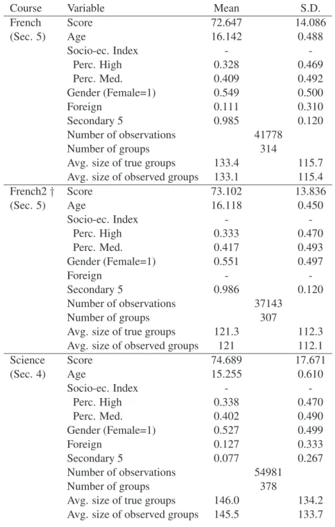
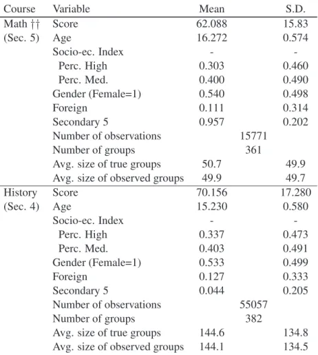
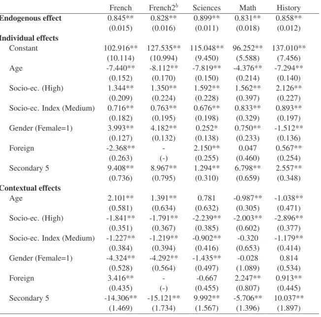
(16) Two test sessions are offered for those who completed coursework in the Spring semester. We thus consider as belonging to the same group all those who belong to the same school and who take a subject test in one of the two consecutive sessions of June and August 2005. We know the number of students in each of these groups. But we only observe test scores for the set of students who took the test in June. Therefore we do not always observe the scores of all students within a group. We offered a correction for this problem in our discussion of the econometric model, and our empirical results below incorporate this correction. In any case an overwhelming majority of the students do take the tests in June, so the correction has little effect on the results. We use for this study French, History, Science and Math test results as reported in the MERS administrative data. Students in a regular track take History and Science tests in Secondary 4. The French test is commonly taken in Secondary 5. For this test only, and because of the obvious impact of language spoken at home, we also look at the subsample of students whose mother tongue and language spoken at home are the same as the language of instruction (French2).24 Finally, we focus on students who take the Math test in Secondary 5 (Math 514). This completes their mathematical training for secondary school.25 We focus on this test in our analysis. We provide descriptive statistics in Table 1. For each subject, the dependent variable in our econometric model is the test score obtained in the provincial standardized test. The average score is between 70% and 75% in French, Science and History tests. It is lower and about 62% in Math. In samples for which the regular track for the test is Secondary 5 (resp. Secondary 4), the average age of students is close to 16 (resp. 15). Most students taking French and Math (98% and 96%) are enrolled in Secondary 5. Most of those taking Science and History are enrolled in Secondary 4 (92% and 96%). Between 52% and 55% of students are female, and between 11% and 13% of students speak a language at home which is different from the language of instruction.26 Between 30 and 34% of students come from a relatively high socioeconomic background and between 40% and 42% from a medium one.27 We observe test scores and characteristics of students taking the same test in June 2005. Sample sizes are 41, 778 for French, 54, 981 for Science, 15, 771 for Math, and 55, 057 for History. When we exclude students 24. Thus, models estimated for this subsample assume that the interaction group is comprised of all other students in the same school qualified to take the test in June 2005 and whose mother tongue and language spoken at home is similar to the language of instruction. 25 The MERS administers a unique test to all secondary school students in French, History and Science. In contrast, it administers different tests in Math, depending on academic options chosen early on by the students. We report here results for students following the regular mathematical training (Math 514). 26 The language of instruction is French in most schools, and English otherwise. 27 We use an index of socio-economic status provided by the MERS. This index is computed from data from the 2001 census. It uses information on the level of education of the mother (a weight of 2/3) and the job status of parents (weight of 1/3). Low socio-economic status corresponds to the three lowest deciles of the index (high socio-economic status to the three highest deciles).. 13.

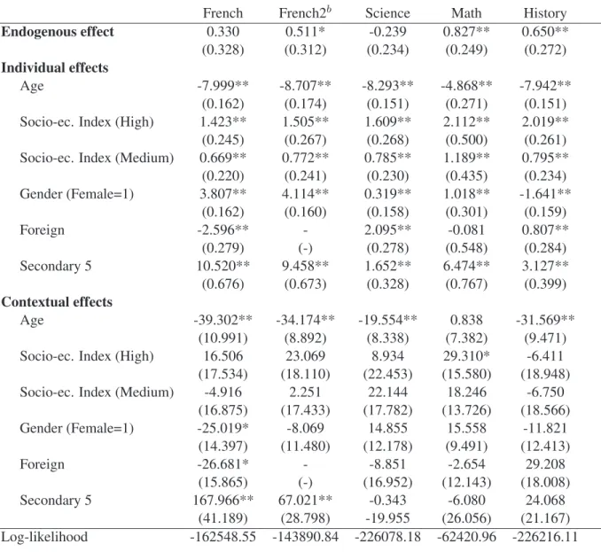
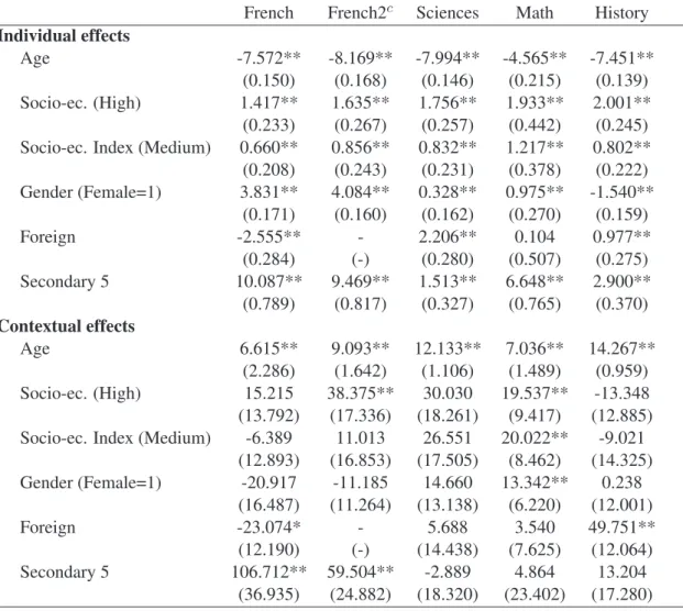
(17) whose mother tongue or language spoken at home is different from the language of instruction, the number of observations for the French sample drops to 37, 143. We also observe the number of students who completed coursework but postpone test-taking to August 2005. There are 118 (89) students postponing French (French2), 186 postponing History, 195 postponing Science, and 160 postponing Math. We observe between 307 and 382 peer groups depending on the subject matter considered. The average group size is between 50 (Math) and 146 (Science). The ratio between the number of groups and the average group size varies between 2.36 (French) and 7.23 (Math). These numbers are relatively small, which suggests that our estimates could be subject to weak identification problems. The group size standard deviation is quite large, however, varying between 50 (in Math) and about 135 (in Science and History). We expect such dispersion in group sizes to help identification. We analyze these issues in more details in Section 6.. 5. Empirical Results. 5.1 Naive estimates We first report naive OLS estimates in Table 2. These estimates provide a useful benchmark with which to compare the results from our more sophisticated methods. We ignore here the two key econometric issues of correlated unobservables and simultaneity, and simply regress individual test score on individual characteristics, average score of peers and average characteristics of peers. So the OLS estimator is not consistent even under the null of no correlated effects. The estimated impact of others’ test scores on one own test score is quite high (about 0.8) and statistically significant for all subjects. Also, most individual and contextual variables are significant. Interestingly, individual and contextual effects corresponding to the same characteristic often have opposite signs. We will see below that many of these features are not robust to addressing the main econometric issues.. 5.2 CML estimates We next report the results of CML estimation in Table 3. The model estimated is the linear-in-means model with group fixed effects, individual impacts, and endogenous and contextual peer effects. We find that the estimated endogenous peer effect lies between −0.24 and 0.83. It is significantly different from zero and positive for ˆ = 0.51), Math (𝛽 ˆ = 0.82), and History (𝛽 ˆ = 0.65). It is not significant for French (𝛽 ˆ = 0.33) and French2 (𝛽 ˆ = −0.23). Note that for all subjects the endogenous effect is smaller that the one obtained using for Science (𝛽 a naive OLS. This is likely to reflect a positive correlation between unobservables and test scores. Such positive correlation could emerge, for instance, from variations in teacher quality. 14.

(18) How do these results compare with those obtained in other studies? As a number of other researchers (e.g., Carrell et al. 2008), we find that the endogenous peer effect on achievement is the largest in Math. This may reflect the fact that Mathematics provide more opportunities for interactions among students. In Math, Hoxby (2000a) reports a 0.1 to 0.55-point increase in own score in relation with a 1-point increase in mean score of peers. Hanushek et al. (2003) show a 0.4-point increase in association with a 1-point increase in mean math score of peers. Zimmer and Toma (2000) report an endogenous math peer effect lying between 0.6 and 0.8. On the lowest side of the spectrum, Vigdor and Nechyba (2004) obtain an endogenous math peer effect of 0.07.28 So our estimate lies on the high side of the range of previous estimates. Most of the individual characteristics have a significant effect on test scores, and the signs of these effects essentially conform to expectations. All test scores decrease significantly with age. Since older students have often repeated a grade, being younger is a natural proxy for ability. Test scores are significantly higher for female students than for male students, except for History where male students perform significantly better than female students. This is broadly consistent with results from previous studies.29 The performance of foreign students is, non surprisingly, significantly lower than for non-foreign students on the French test, but higher for Science and History and not significantly different for Math. Secondary 5 students tend to perform significantly better on all tests than Secondary 4 students, which reflects the positive impact of an additional year of schooling on test scores. Finally, students from a higher socioeconomic category perform significantly better in all tests. Interestingly, estimates of individual effects are close to the ones obtained from naive OLS regressions. However, this is not the case as far as contextual variables are concerned. A few of these variables have a significant impact on student performance. Average age of other students has a negative and significant effect on all test scores except Math where it is positive but not significant. Proportion of other students enrolled in Secondary 5 have a large positive and significant effect on own score in French. Peers’ socioeconomic background has little effect on own schooling performance. When significant, the magnitude of contextual effects is always larger than the magnitude of individual effects. This is not surprising as it captures the effect of a unit change of the characteristic of every other student in the group. Contrary to the OLS estimates, when significant, contextual effects are in general of the same sign as the impact of the individual characteristic to which they are associated.30 This is consistent, for instance, with situations where students work together and may pick up 28. Kang (2007, p. 475) provide a more complete survey of endogenous peer effects in achievement in mathematics. For instance, results from the 2000 Program for International Student Assessment (PISA) show that Quebec female students perform better than males on reading literacy tests but that the differences in performance on mathematics and science tests are smaller and not significant, see Quebec Government (2001). Similarly, in our analysis, the difference in performance is quantitatively large in French but much smaller in the other disciplines. 30 The only exception is the proportion of other female students which has a negative effect on own performance in the French test. 29. 15.

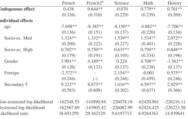
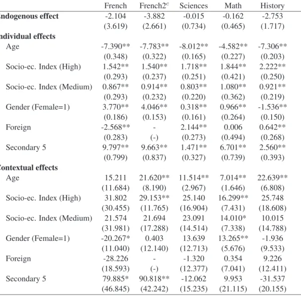
(19) work habits of others. Thus, if older students exert less effort, being in a group with a higher proportion of older students may lead to work less, and this may have a depressing effect on grades independent of the other peer effects.. 5.3 Reflection problem We next take advantage of our framework to examine common ways of getting around the simultaneity problem that do not rely on variations in group sizes. One such way is simply to impose that 𝛽 = 0 (no endogenous effect). Thus, we estimate a model with individual and contextual effects only. In this case the CML estimator is equivalent to a fixed effects OLS estimator. We report results in Table 4. We find that estimated coefficients of individual characteristics are similar to those of the full CML model. However, estimates of contextual effects are quite different. For instance, while a rise in own age is still associated with a decline in own test score, peers’ average age is now found to have a positive and significant effect on own test score for all tests.31 Of course, we know from the CML estimation of the full model that the endogenous effect is significantly different from zero for most subjects. Thus, imposing 𝛽 = 0 is not appropriate here, and the positive age contextual effect is likely picking up the omitted endogenous effect. Note, however, that we need the results from the full estimation to reach this conclusion. Another possible way of addressing the simultaneity problem without exploiting group size variations is to exclude at least one contextual variable from the outcome equation and to use it as an instrument for average test score. We estimate a model similar to the one presented in Table 3 but with no contextual effects (i.e., imposing 𝜹 = 0); see Table 5. Using likelihood ratio tests, we reject the null of no contextual effects for History and the two French samples but not for Science and Math. This suggests that the exclusion restrictions may be valid for these other samples. Therefore, the ML estimators provided in Table 5 should be consistent and asymptotically more efficient than those provided in Table 2 for the Science and Math tests. Observe again, however, that we could not have known this a priori without an estimation of the full model. Overall, this shows the interest of Lee’s solution to the reflection problem. Estimating a model with both endogenous and contextual peer effects is needed to recover precisely the different types of peer effects at work. 31. Note that the results presented in Table 4 cannot be interpreted as the coefficients of the reduced form of the model with endogenous effect. Because of the nonlinear effect of group size on reduced form coefficients, 𝛽 is identified and the reduced forms for cases where 𝛽 = 0 and 𝛽 ∕= 0 differ. This stands in contrast to the analysis in Manski (1993).. 16.

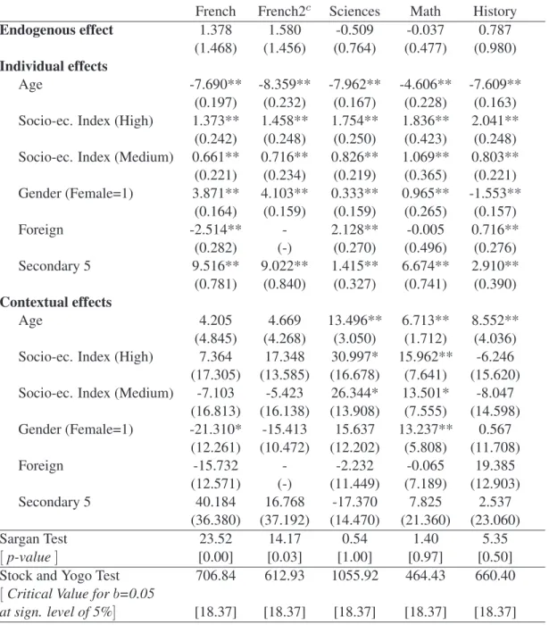
(20) 5.4 2SLS and G2SLS estimates We next contrast IV and CML estimates. We present in Tables 6 and 7 the 2SLS and G2SLS estimation results of the linear-in-means model of peer effects with group fixed effects, individual impacts, and endogenous and contextual peer effects. In contrast to the CML estimates of Table 3, none of the endogenous effects is now statistically significant. This is consistent with Lee’s (2007, p. 345) result that the asymptotic efficiency of IV estimators is smaller than that of the CML. Estimated individual effects are quite similar to the corresponding CML estimates. Some contextual effects are similar while others are different. For instance, the proportion of other students in Secondary 5 still has a large and positive effect on own French score as well as no significant effects for the other subjects. In contrast, average age among peers now has a positive and significant effect on own score for most subjects, rather than a negative one. This could be explained by differences in small sample properties of both methods, possibly aggravated by the imprecision in the estimation of the endogenous peer effect. Table 6 also reports two standard test results giving information on instrumental variables properties. We first look at Sargan tests on the validity of the instruments and the over-identification restrictions of the model. We do not reject the null for Science, Math and History, but we reject it for French (and French2). While this may indicate a problem of model specification in these two last cases, one must be cautious in interpreting the test given the likely low convergence of peer effects IV estimates. We then compute Stock and Yogo (2005)’s test statistics on weak identification.32 Based on the definition that a group of instruments is weak when the bias of the IV estimator relative to the bias of ordinary least squares exceeds a certain threshold 𝑏, say 5%, one rejects the null that the instruments are weak for all subject matters.. 6. Monte Carlo simulations. In this section, we study through simulations the effect of group sizes and their distribution on the precision and bias of our estimates. Lee (2007) shows that the CML and IV estimators may converge in distribution at low rates when the ratio between the number of groups and the average group size is small. Since this ratio varies between 2.36 and 7.23 in our samples, a problem of weak identification could in principle emerge. However, the standard deviation of the distribution of group sizes is also relatively large, and we suspect that this helps identification. To study these issues, we realize two simulation exercices. First, we vary group sizes in a systematic manner 32. The Stock and Yogo test assumes that the instruments are valid, so it may be biased in the case of French and French2.. 17.

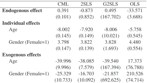
(21) and study how this affects the bias and precision of CML and IV estimators. We notably vary the group size standard deviation and partly calibrate simulation parameters on our data. Second, we look at bias and precision of estimates for fully calibrated simulations, when group sizes are exactly the same as in the data. Overall, while our analysis confirms Lee’s earlier results, we also find a strong positive impact of the standard deviation of group sizes on the strength of identification. Especially, conditional maximum likelihood performs well on fully calibrated simulations. This indicates that the bias due to small sample issues is likely low in the results presented in Table 3. For each simulation exercise, we keep the number of observations fixed around 42, 000, and run 1, 000 replications. We first consider average sizes of 10, 20, 40, 80 and 120. We pick group sizes from the following intervals with decreasing standard deviation: ∙ Average size of 10 : [3, 17], [5, 15], [7, 13] and [9, 11], ∙ Average size of 20 : [3, 37], [8, 32], [13, 27] and [18, 22], ∙ Average size of 40 : [3, 77], [12, 68], [21, 59], [30, 50] and [39, 41], ∙ Average size of 80 : [3, 157], [18, 142], [33, 127], [48, 112] and [63, 97], ∙ Average size of 120 : [3, 237], [28, 212], [53, 187], [78, 162] and [103, 137].. For each of the intervals described above, we proceed in the following manner: 1. pick a group size from a uniform distribution for which the support is defined by the minimum and maximum value of the interval; 2. truncate this value by eliminating its decimal portion; 3. repeat step 1 and 2 as long as the total number of observations is below or equal 42, 000. To reduce computing time, we assume that all students have the same characteristics except for age and gender. We assume that age follows a normal distribution and gender follows a Bernoulli distribution. We calibrate the moments of these distributions on the sample of students taking the French test: average age is 16, variance of age is 0.25, and proportion of girls is 0.55. Values of the structural parameters 𝛽, 𝛾 and 𝛿 are set to. 18.

(22) the estimated coefficients for the French test: 𝛽 = 0.35, 𝛾 𝑎𝑔𝑒 = −8, 𝛾 𝑔𝑒𝑛𝑑𝑒𝑟 = 3.8, 𝛿 𝑎𝑔𝑒 = −40, 𝛿 𝑔𝑒𝑛𝑑𝑒𝑟 = −25. We assume that the values of 𝜖 in the structural equation are drawn randomly from a normal distribution with mean zero and variance 𝜎 2 = 1. We generate the endogenous variable 𝑦 from the reduced-form equation in deviation form. We estimate the model using CML and IV (G2SLS). Looking at Table 8, we first compare simulation results across average group sizes and then we examine how estimators perform for a given average group size as variance in group size decreases. Separate horizontal panels in Table 8 pertain to different values of average group size. We report the average estimated coefficient and standard error by CML and G2SLS for the endogenous effect (first vertical panel), the exogenous effect associated with age (second vertical panel) and the exogenous effect associated with gender (third vertical panel). We find that even for the largest average group size (i.e., 120), both CML and IV perform well in terms of bias and precision (first line in the last horizontal panel of Table 8). The biases of CML and IV get in general larger as average group size increases. The CML estimate of the endogenous effect attains a plateau at the value 1, while the IV estimate becomes rapidly larger (in absolute value) than 1. This is consistent with the fact that the CML estimator tends towards the naive OLS estimator as group sizes become larger. In contrast, the bias on the endogenous effect estimated by IV rapidly exceeds the bias of OLS. This is consistent with instruments becoming less correlated to peer average outcome as group sizes increase. In general, peer effects are also less precisely estimated in large groups than in small groups, regardless of the estimation method. But, for a given Monte Carlo experiment, the magnitude of the bias and the loss in precision are always larger for IV than for CML. Our main new result concerns the effect of group size dispersion. When we fix the value of the average group size and reduce the length of the interval from which group sizes are picked, we find that the bias of both CML and IV typically increases while the precision typically decreases. In Table 8, this amounts to looking at each horizontal panel separately. Since we roughly pick group sizes from a uniform distribution holding average group size fixed, reducing the interval’s length corresponds to a reduction in variance. Not surprisingly, bias of IV rises more rapidly than bias of CML when the variance in group sizes is reduced, and the precision declines more rapidly as well. 19.

(23) We next fully calibrate the simulations’ parameters on the data, We use observed group sizes in the French { } sample, calibrate the model parameters 𝛽, 𝛾 𝑎𝑔𝑒 , 𝛾 𝑔𝑒𝑛𝑑𝑒𝑟 , 𝛿 𝑎𝑔𝑒 , 𝛿 𝑔𝑒𝑛𝑑𝑒𝑟 and moments of the explanatory variables as previously, and set the variance of the error term in the structural model equal to the estimated variance in the French sample (ˆ 𝜎 2 = 154.7). Simulation results are reported in Table 9. The CML estimator has small bias and standard error, while the IV estimator is not precisely estimated and the bias is large. These results confirm what we obtained from picking group sizes at random; they show that dispersion in group sizes help identification. Overall, this suggests that small sample bias may be relatively high in the IV estimates of Tables 6 and 7 but relatively low for the CML estimates of Table 3.. 7. Conclusion. It is now well documented that identification of peer effects on student achievement is challenging because of the difficulties to isolate them from other confounding effects. A number of studies have addressed this problem by exploiting data where students are randomly assigned to groups or by imposing ad hoc exclusion restrictions on the structural model determining student achievement. In this paper, we adopt a different identification strategy. We provide the first empirical application of Lee (2007)’s novel approach, which shows that endogenous and contextual peer effects can be identified when agents interact in groups and when there are sufficient variations in group sizes. Correlated unobservables are allowed as long as they are fixed within each group. The model is applied to original administrative data providing individual scores on standardized tests taken in June 2005 in four subjects by fourth and fifth grade secondary school students in the province of Quebec (Canada). The results generally indicate that students benefit from their peers’ higher test scores. Thus, based on our conditional maximum likelihood results, a point increase in the average test score of his peers increases a student’s test score by 0.5 in French, 0.65 in History and 0.83 in Math. Contextual peer effects also matter. For instance, interacting with older students usually has a negative and significant effect on scores. Overall, our analysis confirm the interest of this new methodology to study peer effects with cross-section observational data. From a practical standpoint, its main limitation is that it needs enough variation in group sizes to perform well. Our Monte-Carlo simulations and empirical results show that the amount of variation present in our data is likely sufficient to obtain reasonable estimates, thank to the typically high variance in school sizes. Our research could be extended in many directions. It would be interesting to evaluate the validity of this approach by using data where group membership is experimentally manipulated and group sizes are heterogenous (as in Sacerdote 2001). Such data would also allow to test the validity of the structural model. It would also be 20.

(24) interesting to analyze how group size variations may help to identify peer effects when the outcome is a discrete variable (e.g., pass or fail). Brock and Durlauf (2001, 2007) have studied peer effects identification with discrete outcomes but they ignore group size variations. A third potentially fruitful direction of research would be to analyze and estimate a nonlinear version of Lee’s approach. For instance, student achievement could depend on the mean and standard deviation of peers’ attributes. Overall, we think that this first empirical application confirmed the interest of the method. Many more applications in different settings are needed, however, in order to gain a thorough understanding of the method’s advantages, limitations, and applicability.. 21.

(25) REFERENCES Ammermueller, A. and Pischke, J-S. (2009): “Peer Effects in European Primary Schools: Evidence from the Progress in International Reading Literacy Study”, Journal of Labor Economics, Vol. 27(3), 315-348. Angrist, J. D. and Lang, K (2004): “Does School Integration Generate Peer Effects? Evidence from Boston’s Metco Program”, American Economic Review, Vol. 94(5), 1613-1634. Angrist, J. D. and Lavy, V. (1999): “Using Maimonides’ Rule to Estimate the Effect of Class Size on Student Achievement”, Quarterly Journal of Economics, Vol. 114(2), 533-575. Atkinson, A., Burgess, S., Gregg, P., Propper, C. and Proud, S. (2008): “The Impact of Classroom Peer Groups on Pupil GCSE Results”, WP no. 08/187, Center for Market and Public Organisation, Bristol, UK. Boozer M. A. and Cacciola, S. E. (2001): “Inside the “Black Box ”of Project STAR: Estimation of Peer Effects Using Experimental Data”, WP no. 832, Economic Growth Center, Yale University. Bramoullé, Y., Djebbari, H. and Fortin, B. (2009): “Identification of Peer Effects Through Social Networks”, Journal of Econometrics, Vol. 150, 41-55. Brock, W. and Durlauf, S. (2001): “Discrete Choice with Social Interactions”, Review of Economic Studies, Vol. 68, 235-260. Brock, W. and Durlauf, S. (2007): “Identification of Binary Choice Models with Social Interactions”. Journal of Econometrics, Vol. 140, 57-75. Burke, M.A. and Sass, T.R. (2008): “Classroom Peer Effects and Student Achievement”, WP no. 18, National Center for Analysis of Longitudinal Data in Education Research. Calvó-Armengol, A., Patacchini, E. and Zenou, Y. (2009): “Peer Effects and Social Networks in Education”, Review of Economic Studies, Vol. 76(4), 1239-1267. Carrel, S.E., Fullerton, R.L. and West. J.E. (2008): “Does Your Cohort Matter? Measuring Peer Effects in College Achievement”,WP no. 14032, National Bureau of Economic Research, Cambridge, MA. Cliff, A. and Ord J. K. (1981): Spatial Processes. London: Pion. Davezies, L., d’Haultfoeuille, X. and Fougère, D. (2009): “Identification of Peer Effects Using Group Size Variation”, Econometric Journal, Vol. 12, 397-413. Evans, W., Oates, W. and Schwab, R. (1992): “Measuring Peer Group Effects: a Study of Teenage Behavior”, Journal of Political Economy, Vol. 100(5), 966-991. Gaviria, A. and Raphael, S. (2001): “School based Peer Effects and Juvenile Behavior”, Review of Economics and Statistics. Vol. 83(2), 257-268. 22.

(26) Glaeser, E., Sacerdote, B. and Scheinkman, J. (1996): “Crime and Social Interaction”, Quarterly Journal of Economics, Vol. CXI, 507-548. Graham, B.S. (2008): “Identifying social interactions through conditional variance restrictions”, Econometrica, Vol. 76 (3), 643-660. Hanushek, E., Kain, J., Markman, J. and Rivkin, S. (2003): “Does Peer Ability Affect Student Achievement?”, Vol. 18(5), Journal of Applied Econometrics, 527-544. Hoxby, C. (2000a): “Peer Effects in the Classroom: Learning from Gender and Race Variation”, WP no. 7867, National Bureau of Economic Research, Cambridge, MA. Hoxby, C. (2000b): “The Effects of Class Size on Student Achievement: New Evidence from Population Variation”, Quarterly Journal of Economics, Vol. 115(4), 1239-1295. Kang, C. (2007): “Classroom Peer Effects and Academic Achievement: Quasi-Randomization Evidence from South Korea”, Vol. 61, Journal of Urban Economics, Vol. 61, 458-495. Kelejian H.H. and Prucha I.R. (1998): “A Generalized Spatial Two-Stage Least Squares Procedure for Estimating a Spatial Autoregressive Model with Autoregressive Disturbances”, Journal of Real Estate Finance and Economics, Vol 17, 99-121. Krueger, A.B. (2003): “Economic Considerations and Class Size”, Economic Journal, Vol. 113(485), F34-F63. Lee, L. F. (2003): “Best Spatial Two-Stage Least Squares Estimators for a Spatial Autoregressive Model with Autoregressive Disturbances”, Econometric Reviews, Vol. 22(4), 307-335. Lee, L. F. (2007): “Identification and Estimation of Econometric Models with Group Interactions, Contextual Factors and Fixed Effects”, Journal of Econometrics, Vol. 140(2), 333-374. Lee, L. F., Liu, X. and Lin X. (2009): “Specification and Estimation of Social Interaction Models with Network Structure, Contextual Factors, Correlation and Fixed Effects”, Econometric Journal, forthcoming. Lin, X. (2008): “Identifying Peer Effects in Student Academic Achievement by Spatial Autoregressive Models with Group Unobservables”, Mimeo, Department of Economics, Tsinghyua University, Beijing. Manski, C. (1993): “Identification of Endogenous Social Effects: The Reflection Problem”, Review of Economic Studies, Vol. 60(3), 531-542. Moffitt, R. (2001): “Policy Interventions, Low-Level Equilibria, and Social Interactions”, in Social Dynamics, edited by Steven Durlauf and Peyton Young, MIT press. Quebec Government. (2001): “PISA 2000. The Performance of Canadian Youth in Reading, Mathematics and Science. Results for Quebec Students Aged 15”, Ministry of Education, Recreation and Sports.. 23.

(27) Rivkin, S. G. (2001): “Tiebout Sorting, Aggregation and the Estimation of Peer Group Effects”, Economics of Education Review, Vol. 20, 201-209. Sacerdote, B. (2001): “Peer Effects with Random Assignment: Results for Darmouth Roommates”, Quarterly Journal of Economics, Vol. 116(2), 681-704. Stinebrickner, R. and Stinebrickner, T. R. (2006): “What Can be Learned About Peer Effects Using College Roommates? Evidence from New Survey Data and Students from Disadvantaged Backgrounds”, Journal of Public Economics, Vol. 90, 1435-1454. Stock, J. H. and Yogo, M. (2005), “Testing for Weak Instruments in Linear IV Regression.”, in Identification and Inference for Econometric Models: Essays in Honor of Thomas J. Rothenberg, edited by D. W. K. Andrews and J. H. Stock, Cambridge University Press. Vigdor, J. L. and Nechyba, T. (2004): “Peer Effects in Elementary Schools: Learning from “apparent”random assignment.”, Mimeo, Department of Economics, Duke University. Zimmer, R. W. and Toma, E. (2000): “Peer Effects in Private and Public Schools Across Countries”, Journal of Policy Analysis and Management, Vol. 19, 75-92. Zimmerman, D. (2003): “Peer Effects in Academic Outcomes: Evidence from a Natural Experiment”, Review of Economics and Statistics, Vol. 85(1), 9-23.. 24.

(28) Table 1: Descriptive statistics Course French (Sec. 5). French2 † (Sec. 5). Science (Sec. 4). Variable Score Age Socio-ec. Index Perc. High Perc. Med. Gender (Female=1) Foreign Secondary 5 Number of observations Number of groups Avg. size of true groups Avg. size of observed groups Score Age Socio-ec. Index Perc. High Perc. Med. Gender (Female=1) Foreign Secondary 5 Number of observations Number of groups Avg. size of true groups Avg. size of observed groups Score Age Socio-ec. Index Perc. High Perc. Med. Gender (Female=1) Foreign Secondary 5 Number of observations Number of groups Avg. size of true groups Avg. size of observed groups. 25. Mean 72.647 16.142 0.328 0.409 0.549 0.111 0.985. S.D. 14.086 0.488 0.469 0.492 0.500 0.310 0.120 41778 314. 133.4 133.1 73.102 16.118 0.333 0.417 0.551 0.986. 115.7 115.4 13.836 0.450 0.470 0.493 0.497 0.120 37143 307. 121.3 121 74.689 15.255 0.338 0.402 0.527 0.127 0.077. 112.3 112.1 17.671 0.610 0.470 0.490 0.499 0.333 0.267 54981 378. 146.0 145.5. 134.2 133.7.