Modeling the Influence of Surface Pitting on Contact
Pressure and Friction Coefficient Under Elastohydrodynamic
Lubrication Conditions
by
Hengameh Sadat MIRKARIMI
THESIS PRESENTED TO ÉCOLE DE TECHNOLOGIE SUPÉRIEURE IN
PARTIAL FULFILLMENT FOR A MASTER’S DEGREE WITH THESIS IN
MECHANICAL ENGINEERING
M.A.Sc.
MONTREAL, JULY 22 2020
ÉCOLE DE TECHNOLOGIE SUPÉRIEURE UNIVERSITÉ DU QUÉBEC
© Copyright reserved
It is forbidden to reproduce, save or share the content of this document either in whole or in parts. The reader who wishes to print or save this document on any media must first get the permission of the author.
BOARD OF EXAMINERS
THIS THESIS HAS BEEN EVALUATED BY THE FOLLOWING BOARD OF EXAMINERS
Mr. Raynald Guilbault, Thesis Supervisor
Mechanical Engineering Department at École de technologie supérieure
Mr. Patrick Terriault, President of the Board of Examiners
Mechanical Engineering Department at École de technologie supérieure
Mr. Tan Pham, Member of the jury
Mechanical Engineering Department at École de technologie supérieure
THIS THESIS WAS PRENSENTED AND DEFENDED
IN THE PRESENCE OF A BOARD OF EXAMINERS AND PUBLIC JULY 14, 2020
ACKNOWLEDGMENT
First and foremost, I would like to express my sincerest gratitude to my supervisor, Professor Raynald Guilbault, for his constant support, patient guidance, and encouragement during my studies. His persistent help and advice have been very helpful to me throughout the completion of my thesis. I have gained so much, not only professionally but also personally, during my study here. This is an experience that will remain with me and inspires me for the rest of my life.
My special thanks are due to my parents, Mostafa and Zhaleh, for their unconditional love, generous support, and continued inspiration. I appreciate all the sacrifices they have done for me. I owe all my success in life to my beloved parents. I, also thank my brother, Foad, and my sister, Talayeh, for their endless love, encouragement, and friendship. Even if we are miles apart, you are always in my heart.
Last but not the least, my heartfelt appreciation goes to my beloved husband, Hossein, who has been always supporting and encouraging me in the moments when there was no one else. Without his devotion, support, and sacrifices, I could have never come this far.
Modélisation de l'influence des piqûres de surface sur les pressions de contact et les coefficients de frottement en régime de lubrification élastohydrodynamique
Hengameh Sadat MIRKARIMI
RÉSUMÉ
Les composants mécaniques utilisés dans les machines sont lubrifiés pour prévenir l’usure et améliorer leur efficacité. La lubrification réduit la génération de chaleur, atténue la pression de surface, et enfin améliore le fonctionnement des équipements. En fonction ses charges externes et des vitesses, différents régimes de lubrification peuvent exister. Plus précisément, le régime élastohydrodynamique décrit le comportement d’un lubrifiant entre surfaces soumises à une charge externes concentrée sur une petite zone de contact, et provoquant des déformations élastiques d’amplitude comparable à l’épaisseur du film de lubrifiant. Ce régime de lubrification apparaît principalement entre des surfaces non conformes.
Les modèles numériques classiques de lubrification élastohydrodynamique ont été développés pour prédire les distributions de pression et les épaisseurs de film de lubrifiant générées entre surfaces lisses ou rugueuses. Cependant, dans des applications réelles, différents types de dégradation peuvent détériorer la qualité des surfaces, et entraîner des changements micro et souvent macroscopiques des conditions de contact.
Les piqûres font partie des défaillances de surface les plus courantes. Ce dommage résulte de chargements cycliques. La présence de piqûres de surface affecte de manière significative les distributions de pression, les épaisseurs de film de lubrifiant et les coefficients de frottement. Ce mémoire s’attelle d’abord à modéliser le contact sec entre deux cylindres. L’approche adoptée s’appuie sur l’algorithme proposé par Hartnet. Cet algorithme est complété par l’ajout de cellules de pression en miroir, combinées au facteur de sur-correction proposé par Guilbault, afin d’éliminer les distributions de contrainte normale et de cisaillement générées sur les surfaces libres. Par la suite, dans le but d’obtenir un modèle élastohydrodynamique pour surfaces lisses, la démarche proposée ajoute l’équation de Reynolds à la solution. La validation du modèle repose sur une comparaison des distributions de pression et épaisseurs de film prédites à des valeurs de référence. Le processus considère différentes conditions de charge et de vitesse. Ensuite, les développements intègrent le terme de l’équation de Reynolds variant dans le temps. Cet élément permet de modéliser des piqûres de surface. L’étude considère différentes profondeurs et configurations de piqûres, afin de comprendre l’influence des défauts de surface sur la lubrification de rouleaux cylindriques. L’analyse compare les réponses obtenues pour des surfaces lisses et dégradées. Les prédictions du modèle numérique confirment que la présence de piqûres affecte de manière importante les pressions de surface, les épaisseurs de film de lubrification, ainsi que les coefficients de frottement.
Mots-clés : Lubrification élastohydrodynamique, pression de surface, épaisseur de film,
Modeling the Influence of Surface Pitting on Contact Pressures and Friction
Coefficients Under Elastohydrodynamic Lubrication Conditions
Hengameh Sadat MIRKARIMI
ABSTRACT
Mechanical components used in machinery are lubricated to prevent wear and enhance their efficiency. Fluid film lubrication reduces heat generation, attenuates surface pressure, and eventually, results in improvements in equipment operation. Depending on external loads and speed, different lubrication regimes may take place. Specifically, the elastohydrodynamic regime describes the lubrication response produced between two mating surfaces sustaining an external load concentrated on a small contact area and causing elastic deformations comparable to the fluid film thickness. This regime of lubrication mainly appears between non-conformal surfaces.
Classical numerical models for elastohydrodynamic lubrication were developed to predict the pressure distributions and the lubricant film thickness profiles generated between smooth or rough surfaces. In addition, in real-world applications, different failure types deteriorate the surface quality and cause micro and even macro changes in the contact conditions.
Pitting is one of the most common surface failures. This damage results from cyclic contact loadings. Surface pits significantly affect pressure distributions, lubricant film thickness, and friction coefficients. In this thesis, we examine the consequences of surface pitting on the line contact problem. The thesis first tackles the modeling of the dry contact between two cylinders. The considered approach is based on the Hartnet algorithm. This algorithm is enhanced by the mirroring of the pressure patches associated with the Guilbault’s overcorrection factor to eliminate the shear and normal stress distributions generated onto the free surfaces. Afterward, the model preparation introduces the Reynolds equation to the solution and form the elastohydrodynamic model for smooth surfaces. The model validation compares the predicted pressure distributions and film thicknesses to reference values. This process considers different loading and speed conditions. Then, the developments integrate the time-variant term of the Reynolds equation into the model. This element allows for modeling surface pits. The study examines different pit depths and arrangements to investigate the influence of surface damages on the lubrication of cylindrical rollers. The analysis compares the response established for smooth and pitted surfaces. The numerical predictions confirm that the introduction of pits significantly affects the surface pressures, the film thicknesses, and the coefficients of friction.
Keywords: Elastohydrodynamic lubrication, surface pressure, film thickness, friction, pitting,
TABLE OF CONTENTS
Page
INTRODUCTION ...1
CHAPTER 1 DRY CONTACT ...9
1.1 Introduction ...9
1.2 Contact problem ...9
1.3 Modeling ...15
1.3.1 Dry Contact Problem ... 15
1.3.2 Mirroring Process... 16
1.3.3 Correction Factor ... 19
1.3.4 Misalignment ... 21
1.4 Conclusion ...27
CHAPTER 2 EHL MODELING ...29
2.1 Introduction ...29 2.2 Reynolds Equation ...29 2.3 Film Thickness ...31 2.4 Lubricant Properties ...33 2.4.1 Lubricant density ... 33 2.4.2 Lubricant viscosity ... 34 2.4.3 Carreau expression ... 34 2.5 Numerical Simulation ...35 2.6 Conclusion ...45
CHAPTER 3 EHL MODELING OF PITTED SURFACES ...47
3.1 Introduction ...47
3.2 Surface pitting failure ...47
3.3 Surface pitting simulation ...48
3.4 Validation-Film thickness and pressure distribution ...52
3.5 Single pit simulation ...57
3.6 Effect of pit depth ...64
3.7 Effect of pit arrangement ...67
3.8 Friction ...75
3.8.1 Validation-Calculation of friction coefficients ... 77
3.8.2 Single pit simulation ... 79
3.8.3 Effect of pit depth ... 81
3.8.4 Effect of pit arrangement ... 82
3.9 Conclusion ...84
RECOMMENDATIONS ...89 LIST OF BIBLIOGRAPHICAL REFERENCES ...91
LIST OF TABLES
Page Table 1.1 Dry contact simulation parameters ...16 Table 3.2 Simulation conditions and dent dimensions-Taken from
(Warhadpande & Sadeghi, 2010) ...53 Table 3.3 Comparison of the pressure profile and film thickness extremums
for the two numerical models ...54 Table 3.4 Experimental (Taken from (Höhn et al., 2006)) and simulation
parameters ...56 Table 3.5 Comparison of the pressure distribution and film thickness extremums
for the experimental measurements and the present model ...57 Table 3.6 Material parameters and problem conditions for single pit simulation ...58 Table 3.7 Rollers and lubricant properties Taken from
LIST OF FIGURES
Page
Figure 0.1 Different lubrication regimes ...1
Figure 0.2 Stribeck curve demonstrating different lubrication regimes Taken from (Chong & De La Cruz, 2014) ...3
Figure 0.3 Schematic conformal and non-conformal mating surfaces Taken from (Shirzadegan, 2016) ...4
Figure 0.4 Pitting failure in a gear-Taken from (“Defects Treated (Gears) |Novexa,” n.d.) ...5
Figure 1.1 (a) Point contact between two spheres (b) Line contact between two cylinders ...10
Figure 1.2 Contact area expansion during load application-Taken from (Collins, 2015) ...10
Figure 1.3 The contact of elastic bodies-Taken from (Hartnett, 1980) ...11
Figure 1.4 Contact of arbitrarily shaped indenters-Taken from (Hartnett, 1980) ...13
Figure 1.5 Numerical solution of dry contact problem ...15
Figure 1.6 Surface Pressure Distribution-right circular cylinder ...16
Figure 1.7 Surface Pressure Distribution-right circular cylinder - 1st step mirroring process...18
Figure 1.8 Surface Pressure Distribution-right circular cylinder - 2nd step mirroring process...18
Figure 1.9 Correction process of quarter-plane free boundary-Taken from (Guilbault, 2011) ...19
Figure 1.10 Surface Pressure Distribution-right circular cylinder-1st step mirroring process-Effect of the correction factor ...20
Figure 1.11 Comparison between different modification methods of pressure distribution correction ...21
Figure 1.12 Two types of misalignments (a) Perpendicular to the contact plane, (b) In contact plane ...22
Figure 1.13 Surface Pressure Distribution-right circular cylinder-1st step mirroring process -0.05 radians misalignment ...23 Figure 1.14 Surface Pressure Distribution-right circular cylinder-1st step mirroring
process and correction factor- 0.05 radians misalignment ...23 Figure 1.15 Surface Pressure Distribution-right circular cylinder-1st step mirroring
process and correction factor - 0.5 radians in-plane misalignment (a) Symmetric view, (b) Top view ...25 Figure 1.16 Surface Pressure Distribution-right circular cylinder-1st step mirroring
process - effect of different radii ...26 Figure 1.17 Surface Pressure Distribution-right circular cylinder-1st step mirroring
process and correction factor - effect of different radii ...27 Figure 2.1 Equivalent contact for the point contact problem -Taken from
(Shirzadegan, 2016) ...32 Figure 2.2 Equivalent contact for the line contact problem-Taken from
(Shirzadegan, 2016) ...32 Figure 2.3 Flowchart of the numerical solution ...37 Figure 2.4 EHL pressure distribution (F = 6000 N, ue = 2.7 m/s) ...38 Figure 2.5 Comparison between dry contact and EHL solution along with the film
thickness (F = 6000 N, ue = 2.7 m/s) ...39 Figure 2.6 Pressure distribution at the midplane of EHL contact for different loads
(ue = 2.7 m/s) ...40 Figure 2.7 Pressure distribution at the midplane of EHL contact for different
rolling speeds (F = 5000 N) ...40 Figure 2.8 Lubricant film thickness (F = 6000 N, ue = 2.7 m/s) ...41 Figure 2.9 Film thickness at the midplane of EHL contact for different loads
(ue = 2.7 m/s) ...42 Figure 2.10 Film thickness at the midplane of EHL contact for different rolling
speeds (F = 5000N) ...42 Figure 2.11 Lubricant viscosity at the midplane of EHL contact for different loads ....43 Figure 2.12 Lubricant viscosity at the midplane of EHL contact for different rolling
XVII
Figure 2.13 Lubricant density at the midplane of EHL contact for different loads ...44
Figure 2.14 Lubricant density at the midplane of EHL contact for different rolling speeds ...45
Figure 3.1 Crater formation for the two pitting types-Taken from (“Polishing - Gear Failures - Failure Atlas - ONYX InSight,” n.d.) ...48
Figure 3.2 Schematic single pit passing through the contact zone ...49
Figure 3.3 Modified flowchart of the numerical solution ...51
Figure 3.4 Pit passing through contact zones ...52
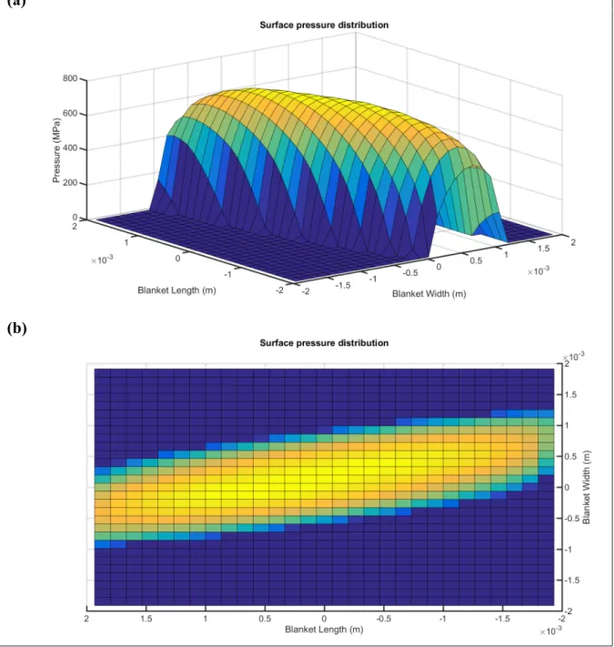
Figure 3.5 Result comparison (a) EHL pressure distribution for the smooth condition, (b) EHL film thickness profile for the smooth condition, (c) EHL pressure distribution for the pitted surface condition, and (d) EHL film thickness profile for the pitted surface condition. ...54
Figure 3.6 Transverse surface texture shape study in (Höhn et al., 2006) ...55
Figure 3.7 Comparing the experimental pressure distribution in (Höhn et al., 2006) with present model ...57
Figure 3.8 3D EHL pressure distribution when the pit position 𝑥𝑝 = −0.78 𝑚𝑚 ...59
Figure 3.9 3D EHL pressure distribution when the pit position 𝑥𝑝 = −0.67 𝑚𝑚 ...60
Figure 3.10 3D EHL pressure distribution when the pit position 𝑥𝑝 = −0.56 𝑚𝑚 ...60
Figure 3.11 3D EHL pressure distribution when the pit position 𝑥𝑝 = 0 ...61
Figure 3.12 3D EHL pressure distribution when the pit position 𝑥𝑝 = 0.27 𝑚𝑚 ...61
Figure 3.13 3D EHL pressure distribution when the pit position 𝑥𝑝 = 0.56 𝑚𝑚 ...62
Figure 3.14 2D EHL pressure distributions at the central axial position of the rollers for the pit locations (a) 𝑥𝑝 = −0.78 𝑚𝑚, (b) 𝑥𝑝 = −0.67 𝑚𝑚, (c) 𝑥𝑝 = −0.56 𝑚𝑚, (d) 𝑥𝑝 = 0, (e) 𝑥𝑝 = 0.27 𝑚𝑚, (f) 𝑥𝑝 = 0.56 𝑚𝑚 ....63
Figure 3.15 Longitudinal pressure distribution in the presence of a single pit passing through the contact zone ...64
Figure 3.16 Effect of pit depth - 2D EHL pressure distributions at the central axial position of the rollers for the pit locations (a) 𝑥𝑝 = −0.78 𝑚𝑚, (b) 𝑥𝑝 = −0.67 𝑚𝑚, (c) 𝑥𝑝 = −0.56 𝑚𝑚, (d) 𝑥𝑝 = 0, (e) 𝑥𝑝 = 0.27 𝑚𝑚, (f) 𝑥𝑝 = 0.56 𝑚𝑚 ...66
Figure 3.17 Multiple pit arrangements ...67
Figure 3.18 3D EHL pressure distribution for the 3-pit configuration ...68
Figure 3.19 3D EHL pressure distribution for the 9-pit configuration ...69
Figure 3.20 3D EHL Film thickness profile for the 3-pit configuration ...69
Figure 3.21 3D EHL Film thickness profile for the 9-pit configuration ...70
Figure 3.22 2D effect of pit configuration at the axial position crossing the central pit - (a) 2D EHL pressure distributions and (b) EHL film thickness profiles ...72
Figure 3.23 Longitudinal pressure distributions calculated along the x = 0 for two multipit configurations ...74
Figure 3.24 Comparing friction coefficient derived from the current model and reference (Najjari & Guilbault, 2014) ...79
Figure 3.25 Effect of a single pit on the friction coefficient (a) Changes in friction coefficient with pit location in the contact zone when SRR = 0.02, (b) Effect of SRR on friction coefficients calculated for the single pit and the smooth surface conditions. ...80
Figure 3.26 Effect of single pit depth on the friction coefficient (a) Changes in friction coefficient with pit location in the contact zone when 𝑆𝑅𝑅 = 0.02, (b) Effect of 𝑆𝑅𝑅 on friction coefficients calculated for single-pit configurations with different depths ...82
Figure 3.27 Effect of pits arrangement on the friction coefficient (a) Changes in friction coefficient with pit location in the contact zone when 𝑆𝑅𝑅 = 0.02, (b) Effect of 𝑆𝑅𝑅 on friction coefficients calculated for different pit arrangements ...84
LIST OF SYMBOLS 𝐴 Contact area 𝑎 Half-length of a cell 𝑏 Half-width of a cell 𝑑 Dent depth 𝑑 Dent width 𝐸 Elastic modulus 𝐸 Equivalent modulus 𝐹 Applied load 𝐹 Friction force 𝑓 Friction coefficient
𝑓 , Flexibility matrix (Influence coefficient relating cell j strip k to cell p strip i) 𝐺 Dimensionless material parameter
𝐺 Lubricant modulus
𝑔 Initial separation of undeformed solids
ℎ Film thickness
ℎ Minimum film thickness
𝐿 Contact length
𝑙 Separation between two circumferential pit rows 𝑙 , 𝑙 Distance from cylinder ends
𝑛 Slope in the lubricant shear-thinning zone
𝑝 Pressure
𝑃∗ Mirror corrected pressure
𝑃 Maximum dry contact pressure 𝑃 Average pressure on cell j strip k
𝑃 Pit depth
𝑃 Pit length
𝑃 Pit width
𝑅 Equivalent radius
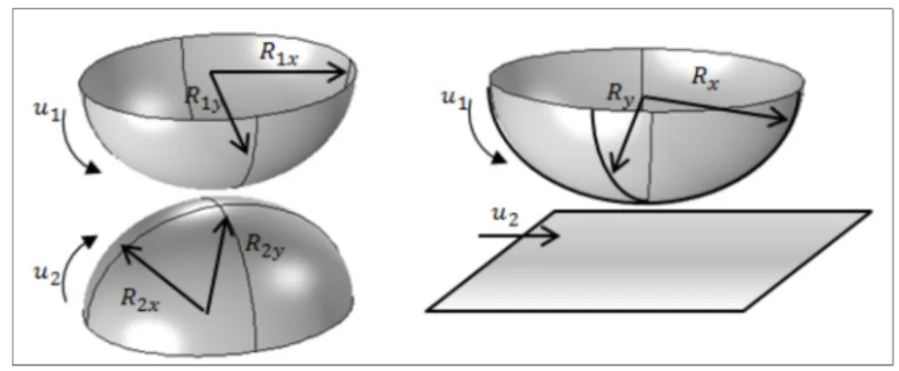
𝑅 , 𝑅 Equivalent radius in x and y directions 𝑅 , 𝑅 Radius of curvature i in x and y directions
𝑆 Dimensionless slope of viscosity-temperature relationship
𝑇 Temperature
𝑇 Ambient temperature
𝑡 Time
𝑈 Dimensionless speed parameter
𝑢 Rolling speed
𝑢 , 𝑢 Velocities of surfaces 1 and 2
𝑤 Total load
𝑊 Dimensionless load parameter
𝑤 Normal displacement of body i
XXI
𝑥 Pit location
𝑥̅, 𝑦 Local coordinate position
𝑧 Dimensionless viscosity-pressure index
𝑧 Separation of body i to plane
𝑧 Separation of body i to plane at the center of cell p 𝛼 Pressure-viscosity coefficient
𝛼 Approach of the bodies
𝛽 Density-temperature coefficient
𝛾 Shear rate
𝛿 Elastic deformation of the contact surfaces
𝛿 Kronecker delta
𝜂 Dynamic viscosity
𝜂 ,𝜂 Shear independent dynamic viscosity
Λ Limiting shear stress-pressure coefficient
𝜈 Poisson’s ratio
𝜌 Density
𝜌 Density at ambient temperature
𝜏 Shear stress
𝜏 Limiting shear stress
INTRODUCTION
Background
In most types of machinery, several rotating or sliding objects are in contact with each other. To reduce friction and wear between sliding surfaces, a substance should be interposed between them. This process is called lubrication. Generally, fluid film lubrication reduces heat generation and moderates contact pressure distribution, which eventually results in a more efficient operation of the equipment. In many mechanical components, such as gears, roller/ball bearings, clutches, and tappet cam mechanisms, contacts take place under various lubrication regimes. Regarding the load and the speed of the contacting surfaces, different lubrication regimes are categorized (Bolander & Sadeghi, 2006) as shown in Figure 0.1.
Figure 0.1 Different lubrication regimes
a. Boundary lubrication
In this mode of lubrication, solid surfaces come into contact mainly at their asperities. Therefore, the surface asperities are considered as the principal load supporters. In this case, the role of the lubricant and its hydrodynamic effects in carrying the load are negligible. Due to the asperities contact, wear and friction are significant in this lubrication regime.
b. Mixed lubrication
The transient regime between boundary lubrication and hydrodynamic lubrication is called mixed lubrication. The solid bodies are not completely separated by the lubricant film, and there are some asperity contacts between the bodies. The hydrodynamic effects of the lubricant are more considerable in this mode. The load is, therefore, being carried by both asperities and
the lubricant film.
c. Elastohydrodynamic lubrication (EHL)
This regime of lubrication is found in nonconforming surfaces and heavy load conditions. Due to these conditions, the elastic strain in the contact area changes the separation of the mating surfaces while the piezo-viscous nature of the lubricant causes the viscosity increases. In other words, the lubricant film thickness in EHL highly depends on a combination of elastic deformation of the solid surfaces and considerable viscosity augmentation through the high-pressure zone. In such conditions, asperity contacts are not completely eliminated but remain sparse.
d. Hydrodynamic lubrication
The main characteristic of hydrodynamic lubrication is that the load is entirely carried by the lubricant film while the mating surfaces are completely separated by the lubricant film. This lubrication regime prevents contacts between solid surfaces. As for the elastohydrodynamic regime, in hydrodynamic lubrication, the motion of the mating surfaces plays the main role in the lubricant flow.
In industry, most contacts are lubricated to control friction and wear. In real applications, such as cylinder liners, piston rings, rolls, and machine tools, contacts operate in a specific lubrication regime. To optimize the contact regarding friction, on the one hand, and lifetime, on the other hand, it is necessary to predict the lubrication regime in which such contacts operate (Gelinck & Schipper, 2000). In lubricated sliding, the friction coefficient during lubrication is potentially influenced by sliding speed, mean contact pressure or normal load, and dynamic viscosity. In the lubrication theory, these three quantities often appear in a single
3
quantity called the Sommerfeld number (𝜂𝑈 𝑝⁄ ) where 𝜂, 𝑈, and 𝑝 correspond to viscosity, velocity and pressure respectively (Gelinck & Schipper, 2000).
Experiments on the lubrication of material surfaces as a function of the Sommerfeld number often reduce to the Stribeck curve (Figure 0.2). Plotting the Stribeck curve is still a convenient method for examining the effect of important variables of sliding speed and normal load to indicate lubrication mechanisms and predict the lubrication regime. EHL friction, sometimes called traction, is important as it is directly associated with machine components performance, efficiency, and energy consumption. This thesis focuses on EHL condition.
Figure 0.2 Stribeck curve demonstrating different lubrication regimes Taken from (Chong & De La Cruz, 2014)
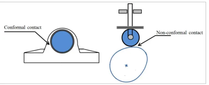
In the analysis of the interaction between mating surfaces, two types of contact can be observed, namely conforming contacts and nonconforming contacts. For the conformal case, the curvatures fit closely together, and the contact area is large before any deformation. On the other hand, in non-conformal contact, the curvatures of the surfaces do not match, and the contact area is small, and the contact pressure and stresses are therefore highly concentrated. (Figure 0.3) EHL mainly appears between nonconformal surfaces.
Figure 0.3 Schematic conformal and non-conformal mating surfaces Taken from (Shirzadegan, 2016)
Although an efficient lubrication regime protects from adhesive and abrasive wear, contact fatigue remains inevitable. Contact fatigue results in micro-pitting and pitting (Guilbault & Lalonde, 2019). This mechanism takes place due to cyclic loadings. Figure 0.4 shows pitted gear surfaces. Based on the crack initiation location, this mode of failure is classified into two categories: surface pitting and subsurface pitting. Pits are formed in all rolling pairs but are particularly common in rolling bearings and gear transmission elements. In such cases, contact takes place under EHL conditions.
Surface defects like pitting can have deleterious effects on the efficiency of lubrication. The EHL theory is a proper method to study pitting failure and its effects. Pitting fatigue has been also studied in a few works over the years. Fatigue life calculation for the pitted surfaces is well studied in the literature. The experimental methods to model surface roughness in EHL conditions, such as light interferometry, have some limitations and difficulties, which is beyond the scope of this thesis. The numerical methods for simulating the topography both in dry contact and EHL conditions are, therefore, more popular. In dry contact condition, the friction between the mating objects plays the most important role in expediting the crack propagation. However, in EHL conditions, the lubricant may penetrate the crack and act as a wedge to form the pits (Datsyshyn & Panasyuk, 2001). In terms of surface pitting simulations, different models can be implemented. An artificial set of pits can be generated in the geometry using sinusoidal patterns (He, Ren, Zhu, & Wang, 2014). Also, a fast Fourier transform (FFT)
5
can be employed to estimate the surface roughness and the pits (S. Liu, Wang, & Liu, 2000). To include more sophisticated patterns, some researchers tended to use two-dimensional (2D) models. Generally, modeling the line contact problem is a 2D problem. However, since the topography of the surface, i.e. the pits and cracks, is three-dimensional (3D), the whole formulation should be 3D to include the effect of the topography (Zhu, Wang, & Ren, 2009).
Figure 0.4 Pitting failure in a gear-Taken from (“Defects Treated (Gears) | Novexa,” n.d.)
Literature review
During the years, several researchers have studied the EHL for different contact surfaces. As the pioneers, Grubin and Vinogradova (1949) investigated EHL theory by considering both elastic deformation and viscosity-pressure effect of the lubricant. Their model describes the mechanical behavior of the mating surfaces assuming that the elastic strain in the loaded region is equal to that of the dry contact problem. Dowson & Higginson (1967) presented a solution for highly loaded line contacts under EHL conditions by considering the film thickness as the dependent variable to the pressure distribution. Hamrock & Dowson (1975) investigated the EHL condition of elliptical contacts by comprehensively studying different loading conditions and material characteristics.
The EHL solution process couples Reynolds equation, elasticity equations, and piezo-viscous lubricant equation leading to numerically complicated problems. Many efforts have been made to find an efficient numerical solution of EHL problems. Different numerical approaches such as direct method, inverse method, quasi-inverse, and system approach methods have been reviewed by Hamrock and Tripp (1984). They presented the advantages and disadvantages of each approach. Okamura (1983) used the Newton-Raphson method to solve the system of finite element equations in the EHL problem. Their results mainly describe the lightly loaded EHL problems. Solutions for highly loaded cases were investigated by Houpert and Hamrock (1986) using adaptive non-uniform meshes to solve the EHL equations. In contrast to practical elements with a finite length such as gears and roller bearings, their solution was limited to infinite line contacts or point contact geometries. (KURODA, S., & ARAI, 1985) combined the finite difference and Newton-Raphson methods to solve the EHL problem for the finite cylindrical rollers. (Park & Kim, 1998) also provided a numerical solution of the EHL problem for the finite line condition. (Najjari & Guilbault, 2014) studied finite line thermal EHL problems for profiled rollers. They considered different roller profile corrections such as chamfered corners, rounded edges, and logarithmic profiles to investigate the edge contact effect on the pressure distribution and the lubricant film thickness.
In the case of experimental studies, (Wymer & Cameron, 1974) tested finite line contacts under the EHL condition. (Mostofi & Gohar, 1983) considered rollers with profiled edge under EHL conditions. Their investigations were, however, limited to low or moderate loads. (Masjedi & Khonsari, 2015) and (Olver & Dini, 2007) independently investigated the effect of surface properties such as roughness on the film thickness and pressure distribution. (Zhu, Ren, & Wang, 2009) used a 3D line contact EHL to predict the gear pitting fatigue life. Using the mixed EHL condition, (Li & Kahraman, 2013) studied the pitting failure modes. (Chue & Chung, 2000) investigated the mechanism of pitting caused by rolling contact using the fracture mechanics approach. They stated that the initial crack and its orientation, indentation force, friction, hydraulic pressure in the crack, and strained-hardened surface layer have critical effects on the pit formation. (Keer & Bryant, 1983) evaluated fatigue lives for rolling/sliding Hertzian contacts using a two-dimensional fracture mechanics approach. They assumed that
7
the crack initiation life is small in comparison to the crack propagation life. (Fajdiga, Glodež, & Kramar, 2007) presented a computational model for the simulation of surface-initiated fatigue crack growth in contacting mechanical elements. As stated before, surface contact failures are very common and much effort has been made to investigate the problem, but progress has been limited due to the complexities in understanding the mechanism of surface pitting effects and the lack of effective ways to estimate friction. Hence, a comprehensive model to investigate the effects of such a surface failure on friction coefficient and contact pressures is needed.
Objectives of the research
As indicated above, this thesis focuses on EHL regime. It particularly concentrates on the influence of fatigue pits on the lubricant film formation. The first objective of the research pertains to developing a comprehensive numerical model to investigate the effects of surface pitting on contact pressures and friction coefficient under EHL conditions. According to this objective, the specific aims are defined as:
• Developing and validating a precise 3D EHL model which describes pitting influence on film thickness and pressure distribution under finite line contact condition
• Integration of free-boundary influence in EHL model
• Investigation of surface pitting impacts on contact pressures and friction coefficients
Thesis organization
This chapter presented an overview of the subject background. It also includes a definition of the research problem and objectives. The chapter also reviews the literature related to numerical modeling of the EHL problem along with the previous experimental studies. Chapter 1 covers the contact problem and dry contact condition and presents the governing system of equations. It also describes the adopted methodology (mirroring method, correction factor, and different types of body misalignments). The investigation results describe the
pressure distributions predicted for different geometries. Chapter 2 covers the EHL model. It presents the governing equations for EHL conditions lubricant density and viscosity. This chapter also displays the film thickness and pressure distribution results predicted for selected systems. The dry contact and EHL models, used in chapters 1 and 2, have been previously introduced by other researchers, and we redeveloped and resolved the problem to make the foundation for modeling the pitting problem. Chapter 3 is dedicated to surface pitting in EHL condition. It describes the equations and models required to incorporate the effect of pitting in EHL as well as the friction coefficient equations. It finally shows the results obtained for various surfaces and operating conditions. The effect of pitting on the pressure distribution, film thickness profile, and the friction coefficient is concluded in the conclusion part. Finally, some future works are proposed in the recommendations section.
CHAPTER 1 DRY CONTACT
1.1 Introduction
Machinery elements consist of various contact systems that are transmitting forces and torques. Except for some specific applications such as pulley and belt systems in which friction is helpful, most of the contact surfaces are lubricated for enhancing the machine efficiency. To study the contact mechanics in lubricated surfaces, specifically in the EHL regime, the dry contact problem should be initially modeled. Our specific aim in this chapter is to derive the pressure distribution under dry contact conditions. This is the first of the essential steps in modeling the EHL contact problem.
1.2 Contact problem
The design and stress analysis of rolling elements is one of the most important topics of mechanical engineering. The lifetime of rolling systems is inversely proportional to the stresses within the contact surfaces. Gears, ball bearing, and roller bearing are some examples of the systems that their lifetime is related to the contact stresses.
As shown in Figure 1, there are two types of contact area between mating rolling surfaces under pre-pressed condition (zero loads):
1. Point contact: The contact between the two rolling solids initiate on a single point, e.g. ball bearings.
(a) (b)
Figure 1.1 (a) Point contact between two spheres (b) Line contact between two cylinders Before loading, the contact area is usually small in both principal directions (point contact condition), or at least in one direction (line contact). However, after applying the load, both types of contact areas change. As shown in Figure 1.2 the point contact expands to an elliptical area and the line contact expands to a rectangle.
Figure 1.2 Contact area expansion during load application-Taken from (Collins, 2015)
11
The first analysis of elastic contact problems was presented by H. (Hertz, 1896). Many other researchers have tried to develop and extend his works to include more loading conditions. In this context, (Hartnett, 1980) presented a numerical procedure to solve the general dry contact problem.
The following describes the algorithm and procedure of Hartnett’s solution. The results of a dry contact problem based on this method are presented. Hartnett considers a pair of three-dimensional nonconforming elastic bodies as the contact surfaces. A schematic of an elastic body contact problem is demonstrated in Figure 1.3.
Figure 1.3 The contact of elastic bodies-Taken from (Hartnett, 1980)
For each object, an independent coordinate system is defined (x1y1z1 and x2y2z2), which have a common origin at the first point of contact. The rules governing the surface displacement is written as in equations (1.1) and (1.2).
𝑤 𝑤 𝑧 𝑧 = 𝛼 (inside the region of contact) (1.1) 𝑤 𝑤 𝑧 𝑧 ≥ 𝛼 (outside the region of contact) (1.2)
Where 𝑧 and 𝑧 are the initial separations, of the bodies from the tangential plan, 𝑤 and 𝑤 represent the bodies’ displacements and 𝛼 stands for the approach of body 1 toward body 2. While solving the equations, two conditions should be satisfied:
1. The pressure distribution in the contact area should result in a total force equal to the applied load.
2. There should be no negative pressure value in the contact zone.
Equations (1.3) and (1.4) formulate these two conditions.
𝑃 𝑥 , 𝑦 𝑑𝑥 , 𝑑𝑦 = 𝐹
Ω
(1.3)
𝑃 𝑥 , 𝑦 ≥ 0 (1.4)
where P stands for the pressure, F is the applied load and 𝑥 , 𝑦 are the coordinates of a position on the contact plane. Eq. (1.3) is called the force balance equation and ensures the equilibrium over the solution domain Ω. In this numerical method, a combination of Boussinesq half-space force-displacement relations and a modified form of the flexibility method are employed. The Hartnett algorithm considers the contact zone as a half-space, and its surface is divided into a system of rectangular cells with piecewise constant contact pressures. Figure 1.4 depicts two arbitrarily shaped surfaces contacting over an area indicated by the shaded zone.
13
Figure 1.4 Contact of arbitrarily shaped indenters-Taken from (Hartnett, 1980)
Solving the systems of linear algebraic equations provides the unknown pressure values. The governing equations are presented below.
𝑤 𝑤 𝑧 𝑧 − 𝑃 𝑓 , 1 − 𝛿 = 𝛼 (1.5)
The elastic deformation of the contact surfaces is 𝛿 𝑥, 𝑦 .
𝛿 𝑥, 𝑦 = 2 𝜋𝐸
𝑝 𝑥 , 𝑦 𝑑𝑥 𝑑𝑦
𝑥 − 𝑥 𝑦 − 𝑦 (1.6)
The discretized contact area into regular cells with uniform pressure results in the following format of the elastic deformation Eq. (1.7) (Najjari & Guilbault, 2014)
𝛿 𝑥, 𝑦 = 2
𝜋𝐸 𝑓 , 𝑝 , (1.7)
𝑃 𝑓 , = 𝐷 (1.8)
𝐷 = 𝛼 − 𝑧 − 𝑧 + 𝑃 𝑓 , 1 − 𝛿 (1.9)
𝑃 ≤ 0 𝑖 = 1,2, … , 𝑛 𝑗 = 1,2, … , 𝑛 (1.10)
where 𝑃 is the constant pressure on a cell, 𝑓 is the influence coefficient, and 𝛿 is the Kronecker delta. Eq. (1.11) gives the influence coefficient.
𝑓 𝑥̅, 𝑦 = 𝑘{ 𝑥̅ + 𝑏 ln 𝑦 + 𝑎 + 𝑦 + 𝑎 + 𝑥̅ + 𝑏 𝑦 − 𝑎 + 𝑦 − 𝑎 + 𝑥̅ + 𝑏 + 𝑦 + 𝑎 ln 𝑥̅ + 𝑏 + 𝑦 + 𝑎 + 𝑥̅ + 𝑏 𝑥̅ − 𝑏 + 𝑦 + 𝑎 + 𝑥̅ − 𝑏 + 𝑥̅ − 𝑏 ln 𝑦 − 𝑎 + 𝑦 − 𝑎 + 𝑥̅ − 𝑏 𝑦 + 𝑎 + 𝑦 + 𝑎 + 𝑥̅ − 𝑏 + 𝑦 − 𝑎 ln ((𝑥̅ − 𝑏 + (𝑦 − 𝑎 + (𝑥̅ − 𝑏 (𝑥̅ + 𝑏 + (𝑦 − 𝑎 + (𝑥̅ + 𝑏 )} (1.11)
a and b represent the dimensions of the rectangular cell and (𝑥̅, 𝑦) are the local coordinate location of the center of cell j regarding the center of cell i, and k is defined as Eq. (1.12)
𝑘 =(1 − 𝜈 )
𝜋𝐸 +
(1 − 𝜈 )
𝜋𝐸 (1.12)
This method incorporates local and remote influence components. The local part is the displacement as the result of loading on the same cell, while the remote component is the displacement induced by the loading on the other cells. In this way, increasing the number of
15
cells provides a proportional increase in the accuracy of the solution. Besides the pressure distribution, the procedure evaluates the contact area and approach of the two bodies.
1.3 Modeling
1.3.1 Dry Contact Problem
The contact area lays onto the plane tangent to the bodies at the initial point or line of contact. By attributing a Cartesian coordinate to this plane, the surface displacement of both bodies is referred to it. The surface is divided into a system of rectangular cells with constant pressure. The unknown pressure values can be determined by solving the system of linear algebraic equations. To initiate the numerical solution, the procedure guesses an initial contact area large enough to include completely the real contact area. (Figure 1.5)
Figure 1.5 Numerical solution of dry contact problem
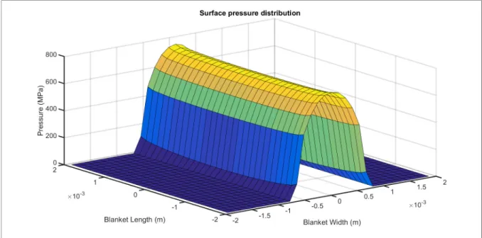
To illustrate the procedure, Figure 1.6 shows the pressure distribution in a contact problem, where two identical right circular cylinders are pressing each other by a contact force of 30 kN. The radius of each cylinder is 10 mm, and the axes of both cylinders are parallel. Table 1.1 shows the simulation parameters of dry contact model. In each cross-section, the maximum
pressure occurs in the centerline of the contact area. The pressure values at the two longitudinal ends of the contact show visible rises. The next section discusses this effect.
Table 1.1 Dry contact simulation parameters
Elastic modulus (E) 200 Gpa Rollers Radius (𝑅 = 𝑅 ) 10 mm
Poisson’s ratio (𝜈) 0.3 Equivalent radius of the rollers (R) 5 mm
Contact force (F) 30 kN Rollers Length (L) 4 mm
Figure 1.6 Surface Pressure Distribution-right circular cylinder
1.3.2 Mirroring Process
Figure 1.6 depicts high-stress concentrations at the edges of the contact area. This numerical phenomenon results from the finite dimensions of the contact bodies. In reality, the free surfaces at the cylinder ends should cause a pressure decrease close to the free edges. The Hartnett algorithm considers both solid bodies as half-space (de Mul, Kalker, & Fredriksson,
17
1986). The half-space theory introduces artificial shear and normal stress distributions on the free surfaces. These stresses increase the rigidity of the cylinder close to their limits. The half-space theory correlates the displacement to the surface tractions (Eqs. (1.7) and (1.9)). The pressure overestimation at the free edges also has a significant effect on the displacement field. To overcome this problem and eliminate the free-boundary artificial shear and normal stress distributions, some correction approaches should be considered. Elimination of normal stress requires computational effort. (de Mul et al., 1986) noted that the shear stress influence is dominant on the surface displacement compared to the normal component. They, therefore, proposed to eliminate the shear contribution.
Mirroring the pressure distribution field regarding the end planes can remove the shear stresses. Repeating this procedure on both sides of the object removes the shear stresses and, therefore, a finite-length solution is achieved. The mirroring process solely removes the shear stresses from the free surfaces. Also, this process doubles the normal stresses at the end planes. The mirroring process can be repeated two or three times until sufficient accuracy is achieved. Figure 1.7 and Figure 1.8 depict the first and the second steps of the mirroring process applied to the contact problem shown in Figure 1.6. The stress concentration at the edges is largely eliminated. Repeating the mirroring process for one more time leads to a minor reduction of the edge stress.
Figure 1.7 Surface Pressure Distribution-right circular cylinder - 1st step mirroring process
19
1.3.3 Correction Factor
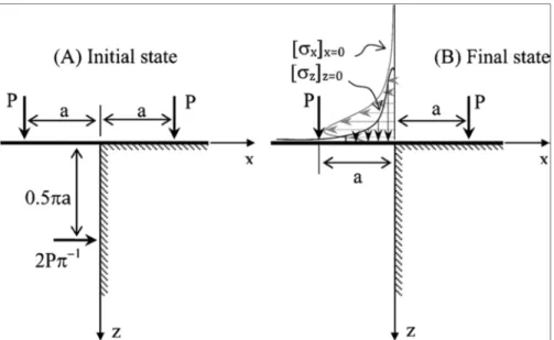
The previous section mentioned that the mirroring process could not remove the normal stresses acting on the free surfaces. (Guilbault, 2011) proposed a correction factor to modify the shear correction procedure to eliminate the normal stresses’ influence on the displacements. To this end, the pressure value of each mirror cell should be multiplied by the Guilbault’s correction factor given by Eq. (1.13), where P and P* are the initial and the mirror corrected pressures, respectively, and ν is the Poisson coefficient. Figure 1.9 Illustrates the quarter-plane free boundary correction operation.
Figure 1.9 Correction process of quarter-plane free boundary-Taken from (Guilbault, 2011)
𝜓 = 𝑃∗
𝑃 = 1.29 − 1
(1 − ν) 0.08 − 0.5ν (1.13)
Applying this method results in a more accurate estimation and causes no modification of the calculation time. Figure 1.10 shows the influence of the correction factor on the previous contact problem. The plot in Figure 1.10 shows a more realistic distribution, where the contact pressure close to the contact ends shows slight decreases, caused the rigidity reduction associated with the free surfaces.
Figure 1.10 Surface Pressure Distribution-right circular cylinder-1st step mirroring process-Effect of the correction factor
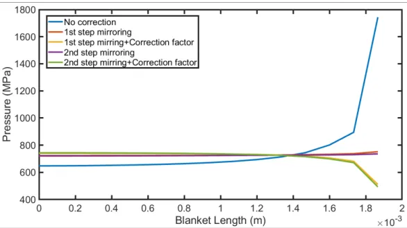
Figure 1.11 compares the pressure distributions resulting from the different correction stages. Although the first mirroring step modifies the pressure distribution, increasing the mirroring steps does not have a remarkable effect. On the other hand, applying the correction factor (Eq. ((1.13)) demonstrates a significant influence.
21
Figure 1.11 Comparison between different modification methods of pressure distribution correction
1.3.4 Misalignment
An ideal loading condition is defined when there is no misalignment between the bodies’ axes. However, the bodies in contact are often subject to a different combination of forces and moments. In practical applications, axial misalignment is common. The mating cylinders may have various types of configurations. Different lengths, tilt, and angularly displacements are examples of cylindrical contact conditions (Figure 1.12). In this context, (Park, 2010) showed that small misalignments have considerable effects on the pressure distributions leading to asymmetric distributions. (Kushwaha, Rahnejat, & Gohar, 2002) studied the misalignment conditions and their influences on the contact between rollers and raceways.
(a) (b)
Figure 1.12 Two types of misalignments (a) Perpendicular to the contact plane, (b) In contact plane
Figure 1.13 displays the pressure distribution calculated for the previous contact problem with 0.05 rad angular misalignment perpendicular to the contact plane (condition (a) in Figure 1.11) when neglecting ψ (Eq.(1.13)). The pressure profile is highly influenced by a tiny tilting condition producing an asymmetric pressure distribution. Applying the Guilbault’s factor to this misalignment problem modifies the pressure distribution at the traction-free edge (Figure 1.14).
23
Figure 1.13 Surface Pressure Distribution-right circular cylinder-1st step mirroring process -0.05 radians misalignment
Figure 1.14 Surface Pressure Distribution-right circular cylinder-1st step mirroring process and correction factor- 0.05 radians misalignment
The pressure distribution related to contact of two cylinders with axes misalignment in contact plane (condition (b) in Figure 1.12) is shown in Figure 1.15 (a). The calculation included Guilbault’s factor (Eq.(1.13)). Figure 1.15 (b) shows the top view of the contact area.
25
(a)
(b)
Figure 1.15 Surface Pressure Distribution-right circular cylinder-1st step mirroring process and correction factor - 0.5 radians in-plane misalignment (a) Symmetric view,
(b) Top view
Figure 1.16 and Figure 1.17 show the pressure distribution for the contact of two cylinders with different radii. In these cases, the axes of both cylinders are parallel, and the radii of the cylinders are 10 mm and 20 mm. Since larger radii increase the contact area, the pressure
values decrease compared to the previous case. The results in Figure 1.16 only include the first step of the mirroring process and neglect the ψ factor. On the other hand, Figure 1.17 shows the pressure distribution when applying the Guilbault’s correction factor.
Figure 1.16 Surface Pressure Distribution-right circular cylinder-1st step mirroring process - effect of different radii
27
Figure 1.17 Surface Pressure Distribution-right circular cylinder-1st step mirroring process and correction factor - effect of different radii
1.4 Conclusion
This chapter showed that numerical methods based on the classic half-space theory are unable to predict the pressure profile of contact areas limited by free surfaces. Rollers of finite length belong to this group. The presented results also demonstrated that applying several steps of mirroring to eliminate the shear stress distribution generated on the free surfaces cannot fully solve this issue. On the other hand, adding the correction factor given by Eq.(1.13) provides precise 3D evaluations of pressure distributions generated between bodies of finite length. While presenting various test cases, this chapter does not include a systematic validation of the dry contact model, since the modeling approach was already fully validated in the reference paper (Guilbault, 2011). Dry contact pressure distributions will be used as the initial values for the EHL solution. The presented model will also establish the elastic deformations of the bodies during EHL simulations.
CHAPTER 2 EHL MODELING
2.1 Introduction
This chapter presents the EHL model prepared to predict lubricant film thicknesses generated between smooth surfaces. It provides the equations for evaluation of lubricant density and viscosity changes caused by pressure variations in lubricant film thickness generated under EHL conditions. The EHL model presented hereafter combines the Hartnett algorithm considering the correction factors discussed in chapter 1 to a finite-difference solution of the 3D Reynolds equation. The modeling strategy described in the following pages is entirely based on the model developed in (Najjari & Guilbault, 2014).
2.2 Reynolds Equation
The governing equations in fluid dynamics (Navier-Stokes and continuity equations) and elasticity equations should be combined to build up a numerical simulation for tribology problems. Accordingly, the Reynolds equation is derived from the 2D Navier-Stokes equation. This formulation includes the following hypotheses:
• The lubricant flow is laminar. • There are no body forces.
• The film thickness is small compared to the dimensions of the contact.
• The lubricant is considered Newtonian with constant density and viscosity across the film thickness.
• A no-slip boundary condition is considered between the lubricant and the surfaces. • The lubricant and the rotating bodies are in isothermal conditions.
Regarding the last assumption, note that the temperature change does not have a significant effect on the pressure and film thickness distributions, specifically when the bodies are rolling
rather than sliding (Y. Liu, 2013). The most important effect of temperature is on the friction coefficient that will be discussed in the next chapter.
A pair of three-dimensional mating solid surfaces with surface velocities of 𝑢 and 𝑢 in the flow direction should be considered. Since the film thickness is assumed to be thin, all derivatives regarding x and y directions are significantly smaller than their equivalents regarding the z-direction. As a result, those smaller terms can be removed to reduce the simulation cost. The Reynolds equation is derived by combining the 2D Navier-Stokes equations to the continuity equation. When neglecting the time derivative component, the Reynolds equation reduces to Eq.(2.1): (Najjari & Guilbault, 2014). Where p represents the pressure, 𝜂 stands for the viscosity, 𝜌 represents the density and 𝑢 =( ) is the velocity.
𝜕 𝜕𝑥 𝜌ℎ 𝜂 𝜕𝑝 𝜕𝑥 + 𝜕 𝜕𝑦 𝜌ℎ 𝜂 𝜕𝑝 𝜕𝑦 = 12𝑢 𝜕(𝜌ℎ) 𝜕𝑥 (2.1)
The Reynolds equation provides pressure distribution throughout the film thickness. The left side terms of this equation are known as “Poiseuille terms” and the right side is called as “Couette term”. Eq. (2.1) is the 3D Reynolds equation. Since we want to simulate the 3D pits and the effect of rollers’ edges, the Reynolds equation in 3D format is used throughout the modeling without any simplification to 2D equation.
It should be mentioned that in the derivation of the above equation the lower surface z1 is chosen as the reference point. The boundary conditions are implemented as follows:
𝑈 = 𝑈 @ 𝑧 = 𝑧 𝑈 = 𝑈 @ 𝑧 = 𝑧
And the velocity profile is expressed as: (Shirzadegan, 2016)
𝑢 = 1 2𝜂 𝜕𝑝 𝜕𝑥(𝑧 − ℎ𝑧) + (𝑢 − 𝑢 ) ℎ (𝑧) + 𝑢 (2.2)
31
The velocity equation consists of two terms: the Poiseuille term which has a parabolic profile and the Couette term with a linear profile.
2.3 Film Thickness
The film thickness equation is given in Eq. (2.3) (Ghosh, 1985)
ℎ(𝑥, 𝑦) = ℎ + 𝑔(𝑥, 𝑦) + 𝛿(𝑥, 𝑦) (2.3)
where ℎ is a constant corresponding to the minimal separation of the two surfaces, 𝑔(𝑥, 𝑦) is the initial separation due to the geometry of the undeformed solids, and 𝛿(𝑥, 𝑦) represents the elastic deformation of the rolling surfaces (calculated with the contact model introduced in Chapter 1). The initial separation of undeformed solids can be written as (Shirzadegan, 2016)
𝑔(𝑥, 𝑦) = 𝑥 2𝑅 +
𝑦
2𝑅 (2.4)
Where 𝑅 and 𝑅 are the reduced radius of curvature in x and y directions depicted in Figure 2.1. (Ghosh, 1985) 1 𝑅 = 1 𝑅 + 1 𝑅 (2.5) 1 𝑅 = 1 𝑅 + 1 𝑅 (2.6)
Figure 2.1 Equivalent contact for the point contact problem -Taken from (Shirzadegan, 2016)
In the case of two aligned rollers in line contact problems, the initial separation reduces to cylindrical-plane contact conditions equivalent to parabolic separations as given below. (Shirzadegan, 2016) 𝑔(𝑥, 𝑦) = 𝑥 2𝑅 (2.7) 1 𝑅 = 1 𝑅 + 1 𝑅 (2.8)
R represents the reduced curvature radius (Figure 2.2).
Figure 2.2 Equivalent contact for the line contact problem-Taken from (Shirzadegan, 2016)
33
The elastic deformation of the rolling surfaces 𝛿(𝑥, 𝑦) is established from the elastic model developed in Chapter 1 for the dry contact conditions.
2.4 Lubricant Properties
Because of the very high pressures involved in EHL contacts, to model those conditions with precision, the compressibility and piezo-viscosity responses of the lubricant should be included in the process.
2.4.1 Lubricant density
Under EHL contact conditions, the lubricant density demonstrates a nonlinear relation with pressure and temperature. A pressure rise causes an increase in the lubricant density. Different expressions formulating the pressure-density were published over the years. The Dowson and Higginson equation is among the most frequently used relations. It includes both the pressure and temperature influence on the lubricant density (Eq. (2.9) below) (Najjari & Guilbault, 2014).
𝜌(𝑝, 𝑇) = 𝜌 [1 + 0.59 × 10 𝑝
1 + 1.17 × 10 𝑝](1 − 𝛽(𝑇 − 𝑇 )) (2.9)
where𝛽, 𝑇, 𝑇 , 𝜌, 𝜌 are the density-temperature coefficient, temperature, ambient temperature, density, and density at ambient temperature, respectively. For constant temperatures, the equation becomes (Shirzadegan, 2016)
𝜌(𝑝) = 𝜌 [0.59 × 10 + 1.34 × 𝑝
2.4.2 Lubricant viscosity
The lubricant viscosity highly depends on pressure and temperature. In EHL contact, the lubricant undergoes intense loading. Therefore, compared to a no-load condition its viscosity may increase several orders of magnitude. This increase in viscosity allows generating lubricant layers sufficiently thick to prevent solid-to-solid contacts and reduce friction and wear. Several models have been proposed to describe the relationship between viscosity, pressure, and temperature. The pressure-viscosity-temperature relation presented by Roelands is probably more accurate. The relation is expressed as (Shirzadegan, 2016)
𝜂(𝑝, 𝑇) = 𝜂 exp {(ln(𝜂 ) + 9.67)[−1 + (1 + 5.1 × 10 p) (𝑇 − 138 𝑇 − 138) ]} (2.11) 𝑧 = 𝛼 5.1 × 10 (ln(𝜂 ) + 9.67) 𝑆 = 𝛽(𝑇 − 138) ln(𝜂 ) + 9.67 2.4.3 Carreau expression
Besides pressure and temperature, shear rates also significantly affect the lubricant viscosity. The relation between the shear stress, viscosity, and shear rate in Newtonian lubricant film can be written as (Shirzadegan, 2016)
𝜏 = 𝜂𝛾 (2.12)
Furthermore, lubricants exhibit a limiting shear stress 𝜏 , over this critical stress, the lubricant shears at a constant stress. The limiting shear stress is linearly proportional to the pressure as written in Eq. (2.14) (Shirzadegan, 2016)
35
𝜏 = 𝜂𝛾 𝜏 < 𝜏𝜏 𝜏 > 𝜏 (2.13)
𝜏 = Λ𝑝 (2.14)
where Λ is the limiting shear stress-pressure coefficient, which has a value of around 0.04-0.08. The rheological model of a non-Newtonian lubricant is thus obtained by implementing Eq. (2.14) into the Carreau expression as shown by Eq. (2.15) (Guilbault, 2013)
𝜂 = min 𝜂 1 + 𝜂 𝐺 𝛾 ( ) ,𝜏 𝛾 (2.15) 2.5 Numerical Simulation
To obtain an appropriate model for the EHL problem, several aspects should be considered. The elastic deformations of rolling surfaces, discretization of lubricant physical model, and finding a proper solution method are the critical steps in deriving the solution. The Reynolds equation is a nonlinear partial differential equation. Moreover, under EHL conditions this relation is coupled with viscosity changes defined by Eqs (2.9), (2.11), and (2.15). As a consequence, it takes some effort to find a stable solution. Actually, to find the pressure distribution and film thickness a system of equations composed of Eq. (2.3), the Reynolds equation, and the force balance must be solved simultaneously.
In this work, the governing equations were discretized along the lubricant film, and a recursive finite difference approach was employed to solve the coupled system of equations. Figure 2.3 presents a flowchart of the algorithm of the numerical solution.
Briefly, the dry contact solution is taken as the initial value for the pressure distribution and ℎ the minimum film thickness is guessed before entering the first loop. Based on these initial values, the material properties of the lubricant are calculated. The discretized Reynolds equation is then solved for the new set of pressures. In the internal loop, by using the newly
calculated pressure set, the surface deformation, film thickness, and lubricant properties are updated. The internal loop should be repeated until the desired accuracy for the pressures is reached. The external loop is dedicated to checking the load balance. As mentioned before, the integration of the pressure value for all the cells in the contact zone should satisfy the equilibrium equation. By adjusting the value for ℎ , one can simply change the load balance conditions. Once both conditions, pressure convergence, and the load balance, were met, the solution is finalized. The numerical modeling and solution were coded in C++. The error limits for pressure distribution and load balance were set to 10 , and the iteration loops were repeated until the calculated parameters falls below the limit of error. The duration of solution procedure was about 1 hour, depending on the total number of cells.
37
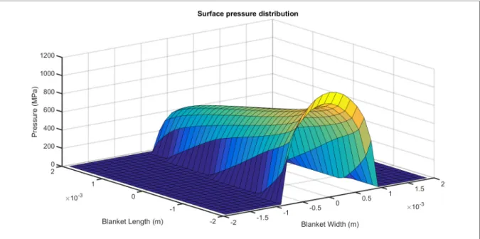
Figure 2.4 presents a 3D visualization of the surface pressure distribution describing the EHL solution obtained for two identical cylindrical rollers of radius 60 mm and parallel axes submitted to an external force of 6000 N and the average entrainment rolling speed of 𝑢 = 2.7 m/s. The calculation includes one mirror level and the ψ factor to release completely the free surfaces at the roller ends. The visible EHL pressure rises close to the cylinder ends assure the mass continuity (in the axial direction) intrinsic to the Reynolds equation (Greenwood & Morales-Espejel, 1995).
To offer a better illustration and compare the results, Figure 2.5 juxtaposes the pressure distributions calculated along the flow direction at the axial central position (pressure cells in the center of the contact area) for both the dry contact and the EHL conditions. The EHL contact region extends toward the input region. The spike in the pressure distribution curve of the EHL maintains the mass continuity (in the flow direction) intrinsic to the Reynolds equation (Greenwood & Morales-Espejel, 1995). The film thickness slope also changes near the point that the spike occurs.
39
Figure 2.5 Comparison between dry contact and EHL solution along with the film thickness (F = 6000 N, u = 2.7 m/s)
To illustrate the effect of external loading on the pressure profile, the problem was modeled using different external forces. As shown in Figure 2.6, the pressure profile for lower forces is more uniform and the spike amplitudes are noticeably smaller. As the force increases, the irregularities in the shape of the pressure profile become more visible. (Elcoate, Evans, & Hughes, 1998) have also reported that when the loading is low, the pressure spike is not visible, and increasing the load generates the spikes. They showed that for very high loadings the spikes become smaller, and in the case of very heavy loadings the simulation gets unstable. The forces that we studied here are almost low loadings (between case 1 and case 2 of (Elcoate et al., 1998), and therefore, the trend is like their case studies. Figure 2.7 depicts the effect of rolling speed, ue, on the pressure distribution. Increasing the value of ue attenuates the spikes in the pressure profile. This trend is in good agreement with the previously reported results (Wolff, Nonaka, Kubo, & Matsuo, 1992).
Figure 2.6 Pressure distribution at the midplane of EHL contact for different loads (u = 2.7 m/s)
Figure 2.7 Pressure distribution at the midplane of EHL contact for different rolling speeds (F = 5000 N)
The most important parameter in EHL modeling is the lubricant film thickness. Figure 2.8 shows the lubricant film thickness profile. Figure 2.9 and Figure 2.10 show the effect of the
41
external force and the relative rolling speed, respectively. As expected, increasing the external force causes a reduction of the lubricant film thickness; the bodies get closer to each other. On the other hand, augmenting the rolling speed increases the lubricant film thickness. Even if these results cannot be generalized, they indicate that the considered rolling speed increase has a more significant influence on the film thickness than the considered external force increase.
Figure 2.9 Film thickness at the midplane of EHL contact for different loads (u = 2.7 m/s)
Figure 2.10 Film thickness at the midplane of EHL contact for different rolling speeds (F = 5000N)
As mentioned before, the lubricant density and viscosity are also affected by pressure changes. Figure 2.11 to Figure 2.14 show the effect of the external force and the rolling speed on these
43
parameters. The viscosity and density profiles are similar to that of the pressure distribution. Augmenting the external force results in visible increases in the lubricant viscosity and density, mostly near the center of the contact zone. On the other hand, the rolling speed has a minimal effect on the lubricant properties.
Figure 2.12 Lubricant viscosity at the midplane of EHL contact for different rolling speeds
45
Figure 2.14 Lubricant density at the midplane of EHL contact for different rolling speeds
2.6 Conclusion
This chapter introduced the EHL calculations for smooth surfaces into the model. It particularly described the influence of external loads and relative rotational velocity on the EHL pressure distribution. The influence of these parameters on the film thickness was also examined. The calculation of the pressure distribution and film thickness presented in this chapter result from a modeling approach put forward in reference (Najjari & Guilbault, 2014). This numerical approach expands the Reynolds equation into its finite differences form over a 2D area representing the lubricated zone. Moreover, since it models smooth surfaces, the adopted form of the Reynolds equation neglects the time derivative term, and hence reduces the problem to a purely geometrical formulation. This solution can now be extended to rollers with pitted surfaces to investigate the effect of this common degradation on pressure distributions and film thickness. Therefore, the next chapter brings back the time derivative component into the solution of the Reynolds equation.
CHAPTER 3
EHL MODELING OF PITTED SURFACES
3.1 Introduction
Surface degradations in rolling contacts affect both the lubrication quality and system efficiency. Specifically, pitting, which is a common type of damage in rolling contact, can drastically alter the pressure distribution profile, the lubricant film thickness, the lubricant viscosity and density, and the coefficient of friction. This chapter adapts the model prepared in the previous chapters to give it the capacity of accounting for the pitting presence. The following investigation also examines the effects of surface pitting on pressure distributions, lubrication quality, and friction. This chapter describes the important contributions of the study, and thus responds to the objective set established in introduction chapter.
3.2 Surface pitting failure
Together with micro-pitting, pitting is one of the principal failure modes occurring in rolling contacts. Pitting is a 3D fatigue phenomenon controlled by the type of cycling contact, the extent of loading, the surface quality, the lubrication nature, the temperature, and the material microstructure. Pitting is generated when a crack is initiated and propagated due to cycling loadings (Fajdiga, Flašker, & Glodež, 2004). Depending on the conditions, pitting can be initiated at surface points or subsurface locations (Figure 3.1).
Under cycling loads, microcracks initiated at subsurface locations may propagate, join each other and reach the surface to form a subsurface initiated pit. Surface initiated microcracks also progress under cycling loadings. However, to propagate and form surface-initiated pits they require additional conditions governed by the lubricant presence and the friction direction. Therefore, only a fraction of microcracks initiated at surface points leads to the formation of debris. The contact fatigue process results in crater formation modifying the mechanical aspect of surfaces. Generally, craters formed by microcracks initiated below the surface are deeper
than those caused by surface-initiated microcracks. The pit formation process is out of the scope of the present study.
The following investigation does not include any contact fatigue modeling or simulation. It instead considers the influence of already formed craters onto the lubrication conditions. The study introduces surface pits by local modifications of the rolling object geometry. In fact, the pitting zones are generated by adjusting the initial distances of the surfaces from the tangent plane at selected points. Combined with the rotational speed of the elements, these surface alterations generate time variations of h in Eq. (2.3) of chapter 2. The original h (x, y) thus becomes h (x, y, t), where g (x, y) introduces the modification.
Figure 3.1 Crater formation for the two pitting types-(“Polishing - Gear Failures - Failure Atlas - ONYX InSight,” n.d.)
3.3 Surface pitting simulation
When ignoring time variations of the lubricant density (ρ), the Reynolds equation presented in chapter 2 (Eq. (2.1)) becomes for pitted surfaces,
𝜕 𝜕𝑥 𝜌ℎ 𝜂 𝜕𝑝 𝜕𝑥 + 𝜕 𝜕𝑦 𝜌ℎ 𝜂 𝜕𝑝 𝜕𝑦 = 12𝑢 𝜕(𝜌ℎ) 𝜕𝑥 + 𝜌 𝜕ℎ 𝜕𝑡 (3.1)
The presence of the additional time term modifies the previous finite difference solution approach since the film thickness now evolves not only because of convergent and divergent