HAL Id: hal-02088494
https://hal.archives-ouvertes.fr/hal-02088494
Submitted on 5 Feb 2020
HAL is a multi-disciplinary open access
archive for the deposit and dissemination of
sci-entific research documents, whether they are
pub-lished or not. The documents may come from
teaching and research institutions in France or
abroad, or from public or private research centers.
L’archive ouverte pluridisciplinaire HAL, est
destinée au dépôt et à la diffusion de documents
scientifiques de niveau recherche, publiés ou non,
émanant des établissements d’enseignement et de
recherche français ou étrangers, des laboratoires
publics ou privés.
Influence of Pseudopotentials on Excitation Energies
From Selected Configuration Interaction and Diffusion
Monte Carlo
Anthony Scemama, Michel Caffarel, Anouar Benali, Denis Jacquemin,
Pierre-Francois Loos
To cite this version:
Anthony Scemama, Michel Caffarel, Anouar Benali, Denis Jacquemin, Pierre-Francois Loos. Influence
of Pseudopotentials on Excitation Energies From Selected Configuration Interaction and Diffusion
Monte Carlo. Results in Chemistry, Elsevier, 2019, 1, pp.100002. �10.1016/j.rechem.2019.100002�.
�hal-02088494�
Configuration Interaction and Diffusion Monte Carlo
Anthony Scemama,1Michel Caffarel,1Anouar Benali,2Denis Jacquemin,3and Pierre-Franc¸ois Loos1,a)
1)Laboratoire de Chimie et Physique Quantiques, Universit´e de Toulouse, CNRS, UPS, France
2)Computational Science Division, Argonne National Laboratory, Argonne, IL 60439, United States of America
3)Laboratoire CEISAM - UMR CNRS 6230, Universit´e de Nantes, 2 Rue de la Houssini`ere, BP 92208, 44322 Nantes Cedex 3, France
Due to their diverse nature, the faithful description of excited states within electronic structure theory methods remains one of the grand challenges of modern theoretical chemistry. Quantum Monte Carlo (QMC) methods have been applied very successfully to ground state properties but still remain generally less effective than other non-stochastic methods for electronically excited states. Nonetheless, we have recently reported accurate excitation energies for small organic molecules at the fixed-node diffusion Monte Carlo (FN-DMC) within a Jastrow-free QMC protocol relying on a deterministic and systematic construction of nodal surfaces using the selected configuration interaction (sCI) algorithm known as CIPSI (Configuration Interaction using a Perturbative Selection made Iteratively). Albeit highly accurate, these all-electron calculations are computationally expensive due to the presence of core electrons. One very popular approach to remove these chemically-inert electrons from the QMC simulation is to introduce pseudopotentials (also known as effective core potentials). Taking the water molecule as an example, we investigate the influence of Burkatzki-Filippi-Dolg (BFD) pseudopotentials and their associated basis sets on vertical excitation energies obtained with sCI and FN-DMC methods. Although these pseudopotentials are known to be relatively safe for ground state properties, we evidence that special care may be required if one strives for highly accurate vertical transition energies. Indeed, comparing all-electron and valence-only calculations, we show that using pseudopotentials with the associated basis sets can induce differences of the order of 0.05 eV on the excitation energies. Fortunately, a reasonable estimate of this shift can be estimated at the sCI level.
I. INTRODUCTION
At the very heart of photochemistry lies the subtle role played by low-lying electronic states and their mutual
interactions.1–5In general, the correct description of these
phe-nomena requires to locate with enough accuracy the first few low-lying excited states of the system and to understand how such states interact not only between themselves (conical in-tersections, spin-orbit effects, ...) but also with other degrees of freedom (coupling with ro-vibrational modes, environment effects, ...). For example, in the case of the photophysics of vision, precious information can be gained by exploring
the excited states of polyenes6–15that are closely related to
rhodopsin which is involved in visual phototransduction.16–21
Accurate and efficient electronic structure methods are now available for the computation of molecular excited states.
Time-dependent density-functional theory (TD-DFT)22is
un-doubtedly at the front of the pack thanks to its favorable cost/accuracy ratio, although several well-documented
short-comings have been put forward in the past twenty years.23–36.
More expensive methods, such as CIS(D),37 CC2,38CC3,39
ADC(2),40 ADC(3),41 EOM-CCSD42(and higher orders CC
approaches43) are also available. Albeit often more
computa-tionally expensive, one can also rely on multiconfigurational methods such as the complete active space self-consistent field
(CASSCF) method,44its second-order perturbation-corrected
variant (CASPT2),45as well as the second-order n-electron
valence state perturbation theory (NEVPT2),46to compute
accurate transition energies. Alternatively to the mainstream
a)Corresponding author: loos@irsamc.ups-tlse.fr
methods mentioned above, selected configuration interaction
(sCI) methods47–50have demonstrated to be valuable
alterna-tives for the computation of highly accurate transition
ener-gies for small molecules.51–67
Pushing further this idea, we have reported, in a recent
study,60accurate excitation energies for two small organic
molecules (water and formaldehyde) using fixed-node
diffu-sion Monte Carlo (FN-DMC)68–73within a Jastrow-free
quan-tum Monte Carlo (QMC) protocol relying on a deterministic and systematic construction of nodal surfaces using the sCI algorithm known as CIPSI (Configuration Interaction using
a Perturbative Selection made Iteratively).49,51–55,59,60,67,74–76.
Within FN-DMC, ensuring accurate calculations of vertical
transition energies is far from being straightforward59,60,77–98
as the mechanism and degree of error compensation of the
fixed-node error99–103in the ground and excited states are
mostly unknown, expect in a few cases.104–111However, our
study has clearly evidenced that the fixed-node errors in the ground and excited states obtained with sCI trial wave func-tions cancel out to a large extent, allowing for the determi-nation of accurate vertical excitation energies for both the singlet and triplet manifolds.
The FN-DMC results reported in Ref. 60 are based on all-electron calculations, i.e., we do not use pseudopotentials (also known as pseudopotentials) to model the core electrons, contrary to what is done in most QMC calculations on large
systems.73,112–114Our motivation was to avoid any
unneces-sary approximation on our excitation energies. However, due to the large fluctuations associated with the very energetic core electrons, all-electron calculations are computationally expensive and must be avoided for large systems. It is then highly desirable to quantify the error that one introduces with pseudopotentials. This problem is investigated here both for
2
Start with|Ψ(0)k i = ∑ I∈D0
c(0)I,k|Ii
Find|αi’s such thathα|Hˆ|Ii 6=0 with|Ii ∈ Diand|αi∈ Di/
Calculate
δE(α)from Eq. (2)
Find|α∗isuch that
δE(α∗) =max α∈AiδE(α) Di+1=Di∪ A∗ i Diagonalize ˆH inDi+1 |Ψ(i+1)k i = ∑ I∈Di+1 c(i+1)I,k |Ii
Exit with|Ψ(n)k iand
perform QMC calculations i←0
Not converged?
i←i+1
Converged? n←i+1
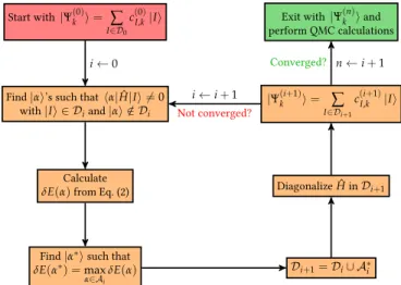
FIG. 1. The CIPSI algorithm. See text for notations.
sCI and DMC calculations using the water molecule as a test system.
This manuscript is organized as follows. The CIPSI algo-rithm used to obtain ground and excited-state wave functions is presented in Sec. II. Computational details are reported in Sec. III. In Sec. IV, we discuss our results and we draw our conclusions in Sec. V. Unless otherwise stated, atomic units are used throughout this study.
II. CIPSI FOR EXCITED STATES
As mentioned above, our sCI method is based on the CIPSI
algorithm.49For a calculation involving Nstates states, the
CIPSI algorithm, represented in Fig. 1, starts with the follow-ing wave functions
|Ψ(0)k i =
∑
I∈D0c(0)
I,k |Ii, (1)
where 0 ≤k ≤ Nstates−1. For a ground-state calculation,
D0is usually taken as the HF determinant only, or a
deter-minant made of natural orbitals obtained from a preliminary calculation. The second option usually significantly speeds up the convergence to the FCI limit. In the case of an
excited-state calculation,D0contains the HF determinant as well as
all single excitations (CIS wave function) and state-averaged natural orbitals are usually employed.
Then, we enter the CIPSI iterative process and look for the
setAiof (external) determinants|αiconnected to the setDi
of (internal) determinants|Ii, i.e. hα|H|Ii 6=ˆ 0.
Next, following Angeli and Persico,117we calculate, using
Epstein-Nesbet perturbation theory, the second-order energy
contribution for each determinant|αiaveraged over all states
δE(α) = Nstates
∑
k cαk maxIc2Ikh Ψ(i)k |H|ˆ αi, (2) with cαk= hΨ (i) k |H|ˆ αi hΨ(i)k |H|ˆ Ψk(i)i − hα|H|ˆ αi. (3) This choice gives a balanced selection between states of dif-ferent multi-configurational nature. We then select thedeter-minants |α∗ihaving the largest contributions, i.e.
δE(α∗) =max
α∈AiδE(α). (4)
The subsetA∗
i ⊂ Aiof determinants |α∗iare then added to
Dito formDi+1, i.e.Di+1=Di∪ A∗i.
This process is repeated until convergence of the ground-and excited-state energies given by the lowest eigenvalues of the Hamiltonian ˆH. At convergence, the CIPSI algorithm provides ground- and excited-state wave functions
|Ψ(n)k i =
∑
I∈DncI,k|Ii(5) that can be used for QMC calculations.
III. COMPUTATIONAL DETAILS
The sCI calculations have been performed with the
elec-tronic structure software qantum package,67 while the
QMC calculations have been performed with the qmc=chem
program.118,119 Both software packages are developed in
Toulouse and are freely available. Our computational pro-cedure follows closely the one reported in Ref. 60, where the interested reader will find additional details about trial wave functions and our Jastrow-free QMC protocol. Be-low, we report more information regarding pseudopotentials.
The ground state geometry of H2O has been obtained at the
CC3/aug-cc-pVTZ level without frozen core approximation. This geometry has been extracted from Ref. 61 and is also
reported assupplementary materialfor sake of completeness.
The sCI calculations have been performed in the frozen-core
approximation with the CIPSI algorithm49which selects
per-turbatively determinants in the FCI space.51–55,59–61,66,74–76
For the calculations involving pseudopotentials, we have used the valence-only Burkatzki-Filippi-Dolg (BFD) cc-pVXZ
basis sets (with X= D, T and Q) in conjunction with the
corresponding BFD small-core pseudopotentials.120,121The
diffuse functions from the standard (all-electron) Dunning basis set family aug-cc-pVXZ were then added to the (diffuse-less) BFD bases. In the following, we labeled as AVXZ and AVXZ-BFD the all-electron Dunning and valence-only BFD bases, respectively.
The FN-DMC simulations are performed using the
stochas-tic reconfiguration algorithm developed by Assaraf et al.,122
with a time-step of 2×10⁻⁴au. In the present case, it is not
necessary to perform time step extrapolations as the time step error is smaller than the statistical error in the computation of excitation energies. Preliminary calculations have shown that
TABLE I. Vertical excitation energies (in eV) for the three lowest singlet and three lowest triplet excited states of water obtained with all-electron AVXZ basis set and with the combination of BFD pseudopotentials and valence-only AVXZ basis sets (X=D, T, and Q). The error
bar corresponding to one standard error is reported in parenthesis. The relative difference between the all-electron and the corresponding pseudopotential calculation is reported in square brackets.
Basis Method Singlet excitations Triplet excitations
1B 1(n → 3s) 1A2(n → 3p) 1A1(n → 3s) 3B1(n → 3s) 3A2(n → 3p) 3A1(n → 3s) AVDZ exFCIa 7.53 9.32 9.94 7.14 9.14 9.48 SHCIb 9.94(1) exDMCa 7.73(1) 9.48(1) 10.10(1) 7.36(1) 9.33(1) 9.63(1) AVDZ-BFD exFCIc 7.48[-0.05] 9.28[-0.04] 9.88[-0.06] 7.07[-0.07] 9.11[-0.03] 9.43[-0.05] SHCIb 9.86(1)[-0.08] exDMCc 7.65(1)[-0.08] 9.45(1)[-0.03] 10.00(1)[-0.10] 7.26(1)[-0.10] 9.27(1)[-0.06] 9.54(1)[-0.09] DMC{J,O}a 9.97(1) AVTZ exFCIa 7.63 9.41 9.99 7.25 9.24 9.54 SHCIb 10.00(0) exDMCa 7.70(2) 9.47(2) 10.05(2) 7.35(1) 9.32(1) 9.61(1) AVTZ-BFD exFCIc 7.58[-0.05] 9.38[-0.03] 9.93[-0.06] 7.16[-0.09] 9.21[-0.03] 9.47[-0.07] SHCIb 9.93(1)[-0.07] exDMCc 7.66(1)[-0.04] 9.49(1)[+0.02] 10.04(1)[-0.01] 7.25(1)[-0.10] 9.30(1)[-0.02] 9.55(1)[-0.06] DMC{J,O}b 10.01(1) AVQZ exFCIa 7.68 9.46 10.03 7.30 9.29 9.58 SHCIb 10.02(1) exDMCa 7.71(1) 9.47(1) 10.03(1) 7.30(1) 9.28(1) 9.59(1) AVQZ-BFD exFCIc 7.63[-0.05] 9.43[-0.03] 9.97[-0.06] 7.21[-0.09] 9.26[-0.03] 9.52[-0.06] SHCIb 9.97(2)[-0.05] exDMCc 7.65(1)[-0.06] 9.45(1)[-0.02] 10.02(1)[-0.01] 7.22(1)[-0.08] 9.24(1)[-0.04] 9.52(1)[-0.07] DMC{J,O}b 10.01(1) CBS exFCIa 7.70 9.48 10.03 7.31 9.30 9.58 exDMCa 7.70(1) 9.46(1) 10.01(1) 7.30(1) 9.28(1) 9.57(1) CBS-BFD exFCIc 7.65[-0.05] 9.46[-0.02] 9.98[-0.05] 7.24[-0.07] 9.28[-0.02] 9.52[-0.06] exDMCc 7.66(1)[-0.04] 9.48(1)[+0.02] 10.04(1)[+0.03] 7.23(1)[-0.07] 9.27(1)[-0.01] 9.53(1)[-0.04] TBEd 7.70 9.47 9.97 7.33 9.30 9.59 Exp.e 7.41 9.20 9.67 7.20 8.90 9.46 aReference 60. bReference 115. cThis work.
dTheoretical best estimates of Ref. 61 obtained from exFCI/AVQZ data corrected with the difference between CC3/AVQZ and CC3/d-aug-cc-pV5Z values. eEnergy loss experiment from Ref. 116.
in the calculation of the excitation energies. This observation is in agreement with the recent results of Blunt and
Neuscam-man on the same system.125As pointed out by Hammond
and coworkers,126when the trial wave function does not
in-clude a Jastrow factor, the non-local pseudopotential can be localized analytically and the usual numerical quadrature over the angular part of the non-local pseudopotential can be es-chewed. In practice, the calculation of the localized part of the pseudopotential represents only a small overhead (about 15%) with respect to a calculation without pseudopotentials (and the same number of electrons). For more details about our implementation of pseudopotentials within QMC, we refer the interested readers to Ref. 127.
IV. RESULTS
A. Selected configuration interaction
Vertical excitation energies for various singlet and triplet states of the water molecule are reported in Table I. For a molecule as small as water (even in a fairly large basis set), it is straightforward to converge sCI calculations and to ob-tain vertical excitation energies with an uncerob-tainty (for a given basis) of 0.01 eV. Throughout the paper, we label these calculations as exFCI (extrapolated FCI) for consistency with
our previous studies.59–61,66In Table I, the relative difference
between the all-electron and the corresponding BFD pseu-dopotential calculations is reported in square brackets. For comparison, we also report the (extrapolated) energies of
Blunt and Neuscamman125obtained with the
semistochas-tic heat-bath CI (SHCI) method,56,57,128one of the other sCI
variants. As expected, these values agree perfectly (within statistical error) with the exFCI energies.
Table I also contains complete basis set (CBS) estimates
obtained with the usual extrapolation formula129
EexFCI(X) =ECBSexFCI+ (X+α1/2)3, (6)
where α and ECBS
exFCIare obtained by fitting the exFCI results
for X= 2 (AVDZ), X= 3 (AVTZ), and X=4 (AVQZ). For
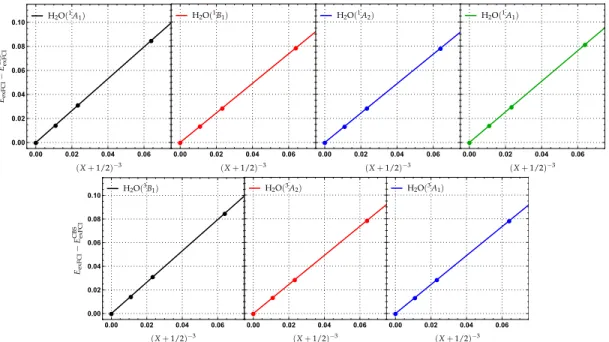
the BFD bases, these fits are represented in Fig. 2 for the four singlet and three triplet transitions studied here. The corresponding all-electron extrapolations can be found in Ref. 60. From Fig. 2, it is clear that these extrapolations can be safely trusted.
At the sCI level, one can clearly see that, for both spin manifolds, the BFD pseudopotentials induce a rather system-atic redshift on the excitation energies of magnitude 0.05 eV (i.e. roughly 1 kcal/mol) which may or may not be an accept-able error depending on the target accuracy. The maximum error is found to be -0.09 eV for the first triplet state whereas
4 ● ● ● ● 0.00 0.02 0.04 0.06 0.00 0.02 0.04 0.06 0.08 0.10 ● ● ● ● 0.00 0.02 0.04 0.06 ● ● ● ● 0.00 0.02 0.04 0.06 ● ● ● ● 0.00 0.02 0.04 0.06 ● ● ● ● 0.00 0.02 0.04 0.06 0.00 0.02 0.04 0.06 0.08 0.10 ● ● ● ● 0.00 0.02 0.04 0.06 ● ● ● ● 0.00 0.02 0.04 0.06
FIG. 2. Extrapolation of the exFCI energies to the complete basis set (CBS) limit for the water molecule. The extrapolated sCI energy EexFCIis
plotted as a function of(X+1/2)−3for X=2 (AVDZ-BFD), X=3 (AVTZ-BFD) and X=4 (AVQZ-BFD). ECBSexFCIstands for the CBS energy
obtained at the exFCI level.
the minimum errors are as small as 0.02–0.03 eV in some cases.
B. Diffusion Monte Carlo
Our ultimate goal is to obtain the FN-DMC energies asso-ciated with the FCI wave functions. However, the ground-and excited-state FCI wave functions are obviously too large to be used as trial wave functions in FN-DMC calculations. Therefore, we use truncated CIPSI expansions (generated as explained in Sec. II) of increasing lengths as trial wave func-tions, and extrapolations are performed in order to estimate the FN-DMC energies one would obtain with the FCI wave functions. In Table II, we report the singlet and triplet exci-tation energies of water obtained at the FN-DMC level for various multideterminantal trial wave functions
ΨT=
Ndet
∑
I cI|Ii
(7)
of size Ndetand variational energy EsCI(where|Iiis a Slater
determinant and cIits corresponding CI coefficient). The
ex-trapolated FN-DMC results, labeled as exDMC and reported in Table I, are obtained by performing a linear extrapolation of
the FN-DMC energy EDMCas a function of EexFCI−EsCIfor
various values of Ndet. Identifying the quantity EexFCI−EsCI
as the variational bias introduced by the truncation of the trial wave function, based on these smaller trial wave
func-tions, we can extrapolate EDMCto EexFCI−EsCI=0 in order
to estimate the FN-DMC energy of the FCI trial wave func-tion. Additional details about this procedure can be found in Refs. 59–61. The graphs associated with these extrapolations
are reported assupplementary materialfor the singlet and
triplet transitions. It is noteworthy that only the last three points are taken into account in the linear extrapolation, i.e., the point corresponding to the smallest trial wave function is systematically discarded.
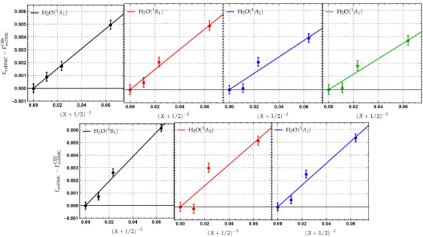
Following a similar procedure as for exFCI (see Sec. IV A), we have performed CBS extrapolations of the exDMC ener-gies. These are represented in Fig. 3. At first sight, it seems that the CBS extrapolations of the exDMC energies are less trustworthy than their variational versions (see Fig. 2). How-ever, it is important to realize that there is a factor of about 16 between the energy scale of the two extrapolation sets in Figs. 2 and 3. In other words, the exDMC extrapolation lines are much flatter than their exFCI counterparts, which does explain their magnified sensitivity. For extra statistics, the two sets of energies can be used altogether as they must extrapolate to the same CBS limit.
At this state, it is worth emphasizing that it is particularly reassuring that, in most cases, the excitation energies obtained at the exFCI and exDMC levels do converge, within statistical error, to the same CBS limit (that is, the exact energy) as it should be. This key observation validates the here-proposed strategy for the CBS extrapolation. However, there is one case
for which it is not true, namely the1A
1(n→3s)transition,
where ECBS
exFCIand ECBSexDMCare significantly different (0.06 eV).
This can be explained by the particularly strong basis set ef-fect associated with the pronounced Rydberg nature of this transition. Indeed, we have recently shown that, even within conventional deterministic wave function methods such as high-level coupled cluster theories, this particular state re-quires doubly-augmented basis sets (d-aug-cc-pVXZ) to be
properly modeled.61
exci-● ● ● ● 0.00 0.02 0.04 0.06 -0.001 0.000 0.001 0.002 0.003 0.004 0.005 0.006 ● ● ● ● 0.00 0.02 0.04 0.06 ● ● ● ● 0.00 0.02 0.04 0.06 ● ● ● ● 0.00 0.02 0.04 0.06 ● ● ● ● 0.00 0.02 0.04 0.06 -0.001 0.000 0.001 0.002 0.003 0.004 0.005 0.006 ● ● ● ● 0.00 0.02 0.04 0.06 ● ● ● ● 0.00 0.02 0.04 0.06
FIG. 3. Extrapolation of the exDMC energies to the complete basis set (CBS) limit for the water molecule. The extrapolated FN-DMC energy EexDMCis plotted as a function of(X+1/2)−3for X=2 (AVDZ-BFD), X=3 (AVTZ-BFD) and X=4 (AVQZ-BFD). ECBSexDMCstands for the CBS energy obtained at the exDMC level.
tation energies gathered in Table I show that the deviation between the all-electron and valence-only results are slightly larger at the FN-DMC level. Yet, this discrepancy is fairly acceptable for usual chemical applications with a maximum error of 0.07 eV, especially knowing the inherent uncertain-ties associated with stochastic simulations. In this regard, we can point out that the excitation energies of Blunt and Neuscamman (obtained with their simple two-determinant ansatz labeled as DMC{J,O} in Table I) seem to benefit from
small, yet systematic, error compensations.125
As a final remark, we would like to point out that, in a large number of cases, we see that the difference between all-electron and pseudopotential calculations can be transferred from the variational to the FN-DMC level. Consequently, if one is able to estimate the error induced by the pseudopoten-tials at the sCI level, it should provide a reasonable estimate of the error that should occur in the FN-DMC excitation energies.
V. CONCLUSION
In the present manuscript, we have reported a preliminary study on the influence of BFD pseudopotentials (and their cor-responding basis sets) on vertical excitation energies obtained at the FN-DMC level with a Jastrow-free protocol. By com-paring valence-only and all-electron calculations performed for six low-lying states of the water molecule, we clearly ev-idence that a small and systematic error is induced by the pseudopotentials and their associated basis set: the transition energy is red-shifted by 0.05 eV at the variational level and slightly more at the FN-DMC level. The similarity between the variational and FN-DMC shifts hints that most of the lo-calization error associated with the use of pseudopotentials
cancels out to a large extent when one computes excitation energies. Hence, the discrepancies between all-electron and valence-only calculations might originate mainly from the difference in the one-electron basis sets. Overall, the small bias introduced by the BFD pseudopotentials and basis sets is acceptable for the vast majority of applications, but could be problematic when looking for very high precision (like in benchmark studies). Finally, we would like to mention that it would be particularly interesting and instructive to test the new generation of pseudopotentials developed by Mitas and
coworkers.130
SUPPLEMENTARY MATERIAL
Seesupplementary materialfor the geometry of the water molecule and the graphs associated with the DMC extrapola-tions.
ACKNOWLEDGMENTS
PFL would like to thank Eric Neuscamman for valuable discussions. Funding from Projet International de Coop´eration
Scientifique(PICS08310) is acknowledged. This work was
per-formed using HPC resources from CALMIP (Toulouse) under allocation 2019-18005 and from GENCI-TGCC (Grant 2018-A0040801738). AB was supported by the U.S. Department of
Energy, Office of Science, Basic Energy Sciences, Materials Sciences and Engineering Division, as part of the Computa-tional Materials Sciences Program and Center for Predictive Simulation of Functional Materials.
6
TABLE II. Vertical excitation energies (in eV) for the three lowest singlet and three lowest triplet excited states of water obtained with the BFD pseudopotentials and the valence-only AVXZ basis sets (X
=D, T, and Q). Ndetis the number of determinants in the trial wave
functions.
Transition AVDZ-BFD AVTZ-BFD AVQZ-BFD Ndet FN-DMC Ndet FN-DMC Ndet FN-DMC 1B 1 8 825 7.67(1) 8 655 7.68(1) 8 856 7.71(1) 65 600 7.66(1) 82 387 7.67(1) 97 937 7.68(1) 287 688 7.65(1) 334 839 7.66(2) 532 734 7.69(1) 646 643 7.65(1) 694 560 7.67(1) 1 579 987 7.63(1) exDMC 7.65(1) 7.66(1) 7.65(1) 1A 2 8 825 9.46(1) 8 655 9.49(1) 8 856 9.47(1) 65 600 9.45(1) 82 387 9.47(1) 97 937 9.48(1) 287 688 9.45(1) 334 839 9.50(2) 532 734 9.49(1) 646 643 9.45(1) 694 560 9.47(1) 1 579 987 9.44(1) exDMC 9.45(1) 9.49(1) 9.45(1) 1A 1 8 825 10.05(1) 8 655 10.07(1) 8 856 10.08(1) 65 600 10.03(1) 82 387 10.03(1) 97 937 10.04(1) 287 688 10.01(1) 334 839 10.02(2) 532 734 10.04(1) 646 643 10.00(1) 694 560 10.04(1) 1 579 987 10.01(1) exDMC 10.00(1) 10.04(1) 10.02(1) 3B 1 5 848 7.23(1) 6 532 7.25(1) 6 446 7.25(1) 51 538 7.24(1) 68 255 7.24(1) 70 637 7.23(1) 289 748 7.25(1) 473 245 7.23(1) 424 318 7.24(1) 1 518 066 7.28(1) 2 128 116 7.25(1) 1 695 420 7.21(1) exDMC 7.26(1) 7.25(1) 7.22(1) 3A 2 5 848 9.23(1) 6 532 9.26(1) 6 446 9.25(1) 51 538 9.29(1) 68 255 9.28(1) 70 637 9.28(1) 289 748 9.29(1) 473 245 9.29(1) 424 318 9.28(1) 1 518 066 9.25(1) 2 128 116 9.29(2) 1 695 420 9.23(1) exDMC 9.27(1) 9.30(1) 9.24(1) 3A 1 5 848 9.54(1) 6 532 9.54(1) 6 446 9.54(1) 51 538 9.55(1) 68 255 9.53(1) 70 637 9.54(1) 289 748 9.54(1) 473 245 9.54(1) 424 318 9.54(1) 1 518 066 9.54(1) 2 128 116 9.53(1) 1 695 420 9.50(1) exDMC 9.54(1) 9.55(1) 9.52(1)
1J. L. Delgado, P.-A. Bouit, S. Filippone, M. Herranz, and N. Mart´ın, Chem. Comm. 46, 4853 (2010).
2K. Palczewski, Ann. Rev. Biochem. 75, 743 (2006).
3F. Bernardi, M. Olivucci, and M. A. Robb, Chem. Soc. Rev. 25, 321 (1996). 4M. Olivucci, Computational Photochemistry (Elsevier Science, Amsterdam;
Boston (Mass.); Paris, 2010).
5M. A. Robb, M. Garavelli, M. Olivucci, and F. Bernardi, “A Computational Strategy for Organic Photochemistry,” in Reviews in Computational Chem-istry, edited by K. B. Lipkowitz and D. B. Boyd (John Wiley & Sons, Inc., Hoboken, NJ, USA, 2007) pp. 87–146.
6L. Serrano-Andr´es, M. Merch´an, I. Nebot-Gil, R. Lindh, and B. O. Roos, J. Chem. Phys. 98, 3151 (1993).
7R. J. Cave and E. R. Davidson, J. Phys. Chem. 92, 614 (1988). 8J. Lappe and R. J. Cave, J. Phys. Chem. A 104, 2294 (2000).
9N. T. Maitra, F. Zhang, R. J. Cave, and K. Burke, J. Chem. Phys. 120, 5932 (2004).
10R. J. Cave, F. Zhang, N. T. Maitra, and K. Burke, Chem. Phys. Lett. 389, 39 (2004).
11M. Wanko, M. Hoffmann, P. Strodel, A. Koslowski, W. Thiel, F. Neese, T. Frauenheim, and M. Elstner, J. Phys. Chem. B 109, 3606 (2005). 12J. H. Starcke, M. Wormit, J. Schirmer, and A. Dreuw, Chem. Phys. 329, 39
(2006).
13C. Angeli, Int. J. Quantum Chem. , 2436 (2010).
14G. Mazur, M. Makowski, R. Wlodarczyk, and Y. Aoki, Int. J. Quantum Chem. 111, 819 (2011).
15M. Huix-Rotllant, A. Ipatov, A. Rubio, and M. E. Casida, Chem. Phys. 391, 120 (2011).
16S. Gozem, F. Melaccio, A. Valentini, M. Filatov, M. Huix-Rotllant, N. Ferr´e, L. M. Frutos, C. Angeli, A. I. Krylov, A. A. Granovsky, R. Lindh, and M. Olivucci, J. Chem. Theory Comput. 10, 3074 (2014).
17M. Huix-Rotllant, B. Natarajan, A. Ipatov, C. Muhavini Wawire, T. Deutsch, and M. E. Casida, Phys. Chem. Chem. Phys. 12, 12811 (2010).
18X. Xu, S. Gozem, M. Olivucci, and D. G. Truhlar, J. Phys. Chem. Lett. 4, 253 (2013).
19I. Schapiro and F. Neese, Comput. Theor. Chem. 1040-1041, 84 (2014). 20D. Tuna, D. Lefrancois, L. Wola´nski, S. Gozem, I. Schapiro, T. Andruni´ow,
A. Dreuw, and M. Olivucci, J. Chem. Theory Comput. 11, 5758 (2015). 21M. Manathunga, X. Yang, H. L. Luk, S. Gozem, L. M. Frutos, A. Valentini,
N. Ferr´e, and M. Olivucci, J. Chem. Theory Comput. 12, 839 (2016). 22M. E. Casida, “Recent advances in density functional methods,” (World
Scientific, Singapore, 1995) p. 155.
23H. L. Woodcock, H. F. Schaefer, and P. R. Schreiner, J. Phys. Chem. A 106, 11923 (2002).
24D. J. Tozer, J. Chem. Phys. 119, 12697 (2003).
25D. J. Tozer, R. D. Amos, N. C. Handy, B. O. Roos, and L. Serrano-Andr´es, Mol. Phys. 97, 859 (1999).
26A. Dreuw, J. L. Weisman, and M. Head-Gordon, J. Chem. Phys. 119, 2943 (2003).
27A. L. Sobolewski and W. Domcke, Chem. Phys. 294, 73 (2003). 28A. Dreuw and M. Head-Gordon, J. Am. Chem. Soc. 126, 4007 (2004). 29N. T. Maitra, J. Phys. Cond. Matt. 29, 423001 (2017).
30D. J. Tozer and N. C. Handy, J. Chem. Phys. 109, 10180 (1998). 31D. J. Tozer and N. C. Handy, Phys. Chem. Chem. Phys. 2, 2117 (2000). 32M. E. Casida, C. Jamorski, K. C. Casida, and D. R. Salahub, J. Chem. Phys.
108, 4439 (1998).
33M. E. Casida and D. R. Salahub, J. Chem. Phys. 113, 8918 (2000). 34E. Tapavicza, I. Tavernelli, U. Rothlisberger, C. Filippi, and M. E. Casida, J.
Chem. Phys. 129, 124108 (2008).
35B. G. Levine, C. Ko, J. Quenneville, and T. J. Mart´ınez, Mol. Phys. 104, 1039 (2006).
36P. Elliott, S. Goldson, C. Canahui, and N. T. Maitra, Chem. Phys. 391, 110 (2011).
37M. Head-Gordon, D. Maurice, and M. Oumi, Chem. Phys. Lett. 246, 114 (1995).
38C. H¨attig and F. Weigend, J. Chem. Phys. 113, 5154 (2000).
39H. Koch, O. Christiansen, P. Jorgensen, A. M. Sanchez de Mer´as, and T. Helgaker, J. Chem. Phys. 106, 1808 (1997).
40A. Dreuw and M. Wormit, WIREs Comput. Mol. Sci. 5, 82 (2015). 41P. H. P. Harbach, M. Wormit, and A. Dreuw, J. Chem. Phys. 141, 064113
(2014).
42G. P. Purvis III and R. J. Bartlett, J. Chem. Phys. 76, 1910 (1982). 43S. A. Kucharski and R. J. Bartlett, Theor. Chim. Acta 80, 387 (1991). 44K. A. B. O. Roos, M. P. Fulscher, P.-A. Malmqvist, and L. Serrano-Andr´es,
“Adv. chem. phys.” (Wiley, New York, 1996) pp. 219–331.
45K. Andersson, P. A. Malmqvist, B. O. Roos, A. J. Sadlej, and K. Wolinski, J. Phys. Chem. 94, 5483 (1990).
46C. Angeli, R. Cimiraglia, and J.-P. Malrieu, Chem. Phys. Lett. 350, 297 (2001).
47C. F. Bender and E. R. Davidson, Phys. Rev. 183, 23 (1969). 48J. L. Whitten and M. Hackmeyer, J. Chem. Phys. 51, 5584 (1969). 49B. Huron, J. P. Malrieu, and P. Rancurel, J. Chem. Phys. 58, 5745 (1973). 50S. Evangelisti, J.-P. Daudey, and J.-P. Malrieu, Chem. Phys. 75, 91 (1983). 51E. Giner, A. Scemama, and M. Caffarel, Can. J. Chem. 91, 879 (2013). 52M. Caffarel, E. Giner, A. Scemama, and A. Ramirez-Solis, J. Chem. Theory
Comput. 10, 5286 (2014).
53E. Giner, A. Scemama, and M. Caffarel, J. Chem. Phys. 142, 044115 (2015). 54Y. Garniron, A. Scemama, P.-F. Loos, and M. Caffarel, J. Chem. Phys. 147,
034101 (2017).
55M. Caffarel, T. Applencourt, E. Giner, and A. Scemama, J. Chem. Phys. 144, 151103 (2016).
56A. A. Holmes, N. M. Tubman, and C. J. Umrigar, J. Chem. Theory Comput. 12, 3674 (2016).
57S. Sharma, A. A. Holmes, G. Jeanmairet, A. Alavi, and C. J. Umrigar, J. Chem. Theory Comput. 13, 1595 (2017).
58A. A. Holmes, C. J. Umrigar, and S. Sharma, J. Chem. Phys. 147, 164111 (2017).
59A. Scemama, Y. Garniron, M. Caffarel, and P. F. Loos, J. Chem. Theory Comput. 14, 1395 (2018).
60A. Scemama, A. Benali, D. Jacquemin, M. Caffarel, and P.-F. Loos, J. Chem. Phys. 149, 034108 (2018).
61P. F. Loos, A. Scemama, A. Blondel, Y. Garniron, M. Caffarel, and D. Jacquemin, J. Chem. Theory Comput. 14, 4360 (2018).
62Y. Garniron, A. Scemama, E. Giner, M. Caffarel, and P. F. Loos, J. Chem. Phys. 149, 064103 (2018).
63F. A. Evangelista, J. Chem. Phys. 140, 124114 (2014).
64J. B. Schriber and F. A. Evangelista, J. Chem. Phys. 144, 161106 (2016). 65P. M. Zimmerman, J. Chem. Phys. 146, 104102 (2017).
66P. F. Loos, M. Boggio-Pasqua, A. Scemama, M. Caffarel, and D. Jacquemin, J. Chem. Theory Comput. 15, in press (2019).
67Y. Garniron, K. Gasperich, T. Applencourt, A. Benali, A. Fert´e, J. Paquier, B. Pradines, R. Assaraf, P. Reinhardt, J. Toulouse, P. Barbaresco, N. Renon, G. David, J. P. Malrieu, M. V´eril, M. Caffarel, P. F. Loos, E. Giner, and A. Scemama, J. Chem. Theory Comput. submitted (2019).
68M. H. Kalos, D. Levesque, and L. Verlet, Phys. Rev. A 9, 2178 (1974). 69D. M. Ceperley and M. H. Kalos, “Monte carlo methods in statistical physics,”
(Springer Verlag, Berlin, 1979).
70P. J. Reynolds, D. M. Ceperley, B. J. Alder, and W. A. Lester, J. Chem. Phys. 77, 5593 (1982).
71W. M. C. Foulkes, R. Q. Hood, and R. J. Needs, Phys. Rev. B 60, 4558 (1999). 72W. A. Lester, L. Mitas, and B. Hammond, Chem. Phys. Lett. 478, 1 (2009). 73B. M. Austin, D. Y. Zubarev, and W. A. Lester, Chem. Rev. 112, 263 (2012). 74A. Scemama, T. Applencourt, E. Giner, and M. Caffarel, J. Chem. Phys.
141, 244110 (2014).
75A. Scemama, T. Applencourt, E. Giner, and M. Caffarel, J. Comput. Chem. 37, 1866 (2016).
76M. Dash, S. Moroni, A. Scemama, and C. Filippi, J. Chem. Theory Comput. 14, 4176 (2018).
77J. C. Grossman, M. Rohlfing, L. Mitas, S. G. Louie, and M. L. Cohen, Phys. Rev. Lett. 86, 472 (2001).
78A. R. Porter, M. D. Towler, and R. J. Needs, Phys. Rev. B 64, 035320 (2001). 79A. R. Porter, O. K. Al-Mushadani, M. D. Towler, and R. J. Needs, J. Chem.
Phys. 114, 7795 (2001).
80A. Puzder, A. J. Williamson, J. C. Grossman, and G. Galli, Phys. Rev. Lett. 88, 097401 (2002).
81A. J. Williamson, J. C. Grossman, R. Q. Hood, A. Puzder, and G. Galli, Phys. Rev. Lett. 89, 196803 (2002).
82A. Aspuru-Guzik, O. El Akramine, J. C. Grossman, and W. A. Lester, J. Chem. Phys. 120, 3049 (2004).
83F. Schautz, F. Buda, and C. Filippi, J. Chem. Phys. 121, 5836 (2004). 84A. Bande, A. L¨uchow, F. Della Sala, and A. G¨orling, J. Chem. Phys. 124,
114114 (2006).
85T. Bouabc¸a, N. Ben Amor, D. Maynau, and M. Caffarel, J. Chem. Phys. 130, 114107 (2009).
86W. Purwanto, S. Zhang, and H. Krakauer, J. Chem. Phys. 130, 094107 (2009).
87P. M. Zimmerman, J. Toulouse, Z. Zhang, C. B. Musgrave, and C. J. Umrigar, J. Chem. Phys. 131, 124103 (2009).
88M. Dubeck´y, R. Derian, L. Mitas, and I. ˇStich, J. Chem. Phys. 133, 244301 (2010).
89R. Send, O. Valsson, and C. Filippi, J. Chem. Theory Comput. 7, 444 (2011). 90R. Guareschi and C. Filippi, J. Chem. Theory Comput. 9, 5513 (2013). 91R. Guareschi, F. M. Floris, C. Amovilli, and C. Filippi, J. Chem. Theory
Comput. 10, 5528 (2014).
92N. Dupuy, S. Bouaouli, F. Mauri, S. Sorella, and M. Casula, J. Chem. Phys. 142, 214109 (2015).
93H. Zulfikri, C. Amovilli, and C. Filippi, J. Chem. Theory Comput. 12, 1157 (2016).
94R. Guareschi, H. Zulfikri, C. Daday, F. M. Floris, C. Amovilli, B. Mennucci, and C. Filippi, J. Chem. Theory Comput. 12, 1674 (2016).
95N. S. Blunt and E. Neuscamman, J. Chem. Phys. 147, 194101 (2017). 96P. J. Robinson, S. D. Pineda Flores, and E. Neuscamman, J. Chem. Phys.
147, 164114 (2017).
97J. A. R. Shea and E. Neuscamman, J. Chem. Theory Comput. 13, 6078 (2017). 98L. Zhao and E. Neuscamman, J. Chem. Theory Comput. 12, 3719 (2016). 99D. M. Ceperley, J. Stat. Phys. 63, 1237 (1991).
100D. Bressanini, D. M. Ceperley, and P. Reynolds, in Recent Advances in Quantum Monte Carlo Methods, Vol. 2, edited by W. A. Lester Jr., S. M. Rothstein, and S. Tanaka (World Scientfic, 2001).
101K. Rasch and L. Mitas, Chem. Phys. Lett. 528, 59 (2012).
102K. M. Rasch, S. Hu, and L. Mitas, J. Chem. Phys. 140, 041102 (2014). 103A. H. Kulahlioglu, K. Rasch, S. Hu, and L. Mitas, Chem. Phys. Lett. 591,
170 (2014).
104M. Bajdich, L. Mitas, G. Drobny, and L. K. Wagner, Phys. Rev. B 72, 075131 (2005).
105D. Bressanini and G. Morosi, J. Chem. Phys. 129, 054103 (2008). 106T. C. Scott, A. L¨uchow, D. Bressanini, and J. D. Morgan, Phys. Rev. A 75,
060101 (2007).
107D. Bressanini and P. J. Reynolds, Phys. Rev. Lett. 95, 110201 (2005). 108D. Bressanini, G. Morosi, and S. Tarasco, J. Chem. Phys. 123, 204109 (2005). 109D. Bressanini, Phys. Rev. B 86, 115120 (2012).
110L. Mitas, Phys. Rev. Lett. 96, 240402 (2006).
111P.-F. Loos and D. Bressanini, J. Chem. Phys. 142, 214112 (2015). 112M. Dubeck´y, L. Mitas, and P. Jureˇcka, Chem. Rev. 116, 5188 (2014). 113A. Benali, N. Shulenburger, L. Romero, J. Kim, and O. von Lilienfeld, J.
Chem. Theory Comp. 10, 3417 (2014).
114A. Ambrosetti, D. Alf`e, R. A. DiStasio Jr., and A. Tkatchenko, J. Phys. Chem. Lett. 5, 849 (2014).
115N. S. Blunt, J. Chem. Phys. 148, 221101 (2018).
116K. Ralphs, G. Serna, L. R. Hargreaves, M. A. Khakoo, C. Winstead, and V. McKoy, J. Phys. B 46, 125201 (2013).
117C. Angeli and M. Persico, Theor. Chem. Acc. 98, 117 (1997).
118A. Scemama, E. Giner, T. Applencourt, and M. Caffarel, “Qmc=chem,” (2017), https://github.com/scemama/qmcchem.
119A. Scemama, M. Caffarel, E. Oseret, and W. Jalby, J. Comput. Chem. 34, 938 (2013).
120M. Burkatzki, C. Filippi, and M. Dolg, J. Chem. Phys. 126, 234105 (2007). 121M. Burkatzki, C. Filippi, and M. Dolg, J. Chem. Phys. 129, 164115 (2008). 122R. Assaraf, M. Caffarel, and A. Khelif, Phys. Rev. E 61, 4566 (2000). 123M. Casula, Phys. Rev. B 74, 161102 (2006).
124M. Casula, S. Moroni, S. Sorella, and C. Filippi, J. Chem. Phys. 132, 154113 (2010).
125N. S. Blunt and E. Neuscamman, J. Chem. Theory Comput. 15, 178 (2019). 126B. L. Hammond, P. J. Reynolds, and W. A. Lester, J. Chem. Phys. 87, 1130
(1987).
127M. Caffarel, T. Applencourt, E. Giner, and A. Scemama, “Using cipsi nodes in diffusion monte carlo,” in Recent Progress in Quantum Monte Carlo (2016) Chap. 2, pp. 15–46.
128J. Li, M. Otten, A. A. Holmes, S. Sharma, and C. J. Umrigar, J. Chem. Phys. 149, 214110 (2018).
129T. Helgaker, P. Jørgensen, and J. Olsen, Molecular Electronic-Structure Theory(John Wiley & Sons, Inc., 2013).
130M. C. Bennett, C. A. Melton, A. Annaberdiyev, G. Wang, L. Shulenburger, and L. Mitas, J. Chem. Phys 147, 224106 (2017).