HAL Id: hal-01433283
https://hal-mines-paristech.archives-ouvertes.fr/hal-01433283
Submitted on 12 Jan 2017
HAL is a multi-disciplinary open access
archive for the deposit and dissemination of
sci-entific research documents, whether they are
pub-lished or not. The documents may come from
teaching and research institutions in France or
abroad, or from public or private research centers.
L’archive ouverte pluridisciplinaire HAL, est
destinée au dépôt et à la diffusion de documents
scientifiques de niveau recherche, publiés ou non,
émanant des établissements d’enseignement et de
recherche français ou étrangers, des laboratoires
publics ou privés.
Wilson-Dirac Operator Revisited on Multicore Vector
Computers
Claude Tadonki
To cite this version:
Claude Tadonki. Wilson-Dirac Operator Revisited on Multicore Vector Computers. [Research Report]
Mines ParisTech - PSL Research University - Centre de Recherche en Informatique (CRI). 2016.
�hal-01433283�
Wilson-Dirac Operator Revisited on Multicore
Vector Computers
Claude Tadonki
Mines ParisTech - PSL Research University Centre de Recherche en Informatique (CRI) 35, rue Saint-Honor´e, 77305, Fontainebleau Cedex (France)
Email: [email protected]
Abstract—We revisit the Wilson-Dirac operator, also refered as Dslash, on multicore vector machines. The Wilson-Dirac operator is the major computing kernel in Lattice Quantum ChromoDynamics (LQCD), which is the canonical discrete for-malism for Quantum ChromoDynamics (QCD) investigations. QCD is the theory of sub-nuclear particles physics, aiming at modeling the strong nuclear force, which is responsible for the interactions of nuclear particles. Based on LQCD formalism, intensive simulations are performed following the Monte Carlo paradigm. Informative observations are expected from large-scale and numerically sensitive LQCD simulations. The corresponding computing demand is therefore tremendous, thus the serious consideration for powerful supercomputers. Designing efficient LQCD codes on modern (mostly hybrid) supercomputers requires to efficiently exploit all available levels of parallelism including accelerators. Since the Wilson-Dirac operator is a coarse-grain stencil computation performed on huge volume of data, any performance and scalability related investigation should skillfully address memory accesses and interprocessor communication overheads. In order the lower the latter, an explicit shared memory implementation should be considered at the node level, since this will lead to a less complex data communication graph. This the main focus of the current paper, where we provide, explain, and discuss a multi-threaded vector implementation, whose experimental results in double precision on the recently released INTEL BROADWELL based machine show a competitive absolute efficiency and a good scalability on one of its four NUMA nodes. An extension to all available nodes is currently under investigation through NUMA-awareness consideration.
545 cuba050new.aketitle
I. INTRODUCTION
Quantum ChromoDynamics (QCD) [21], the theory of the strong nuclear force, can be numerically simulated on massively parallel supercomputers using the Monte Carlo paradigm and the lattice gauge theory (LQCD) approach (see Vranas et al. [20]).
A typical LQCD simulation workflow iteratively involves basic linear algebra computations on a huge number of vari-ables. The major LQCD kernel is the inversion of the Dirac operator, which is an important step during the synthesis of a statistical gauge configuration sample. Indeed, in the Hybrid Monte Carlo (HMC) algorithm [18], it appears in the expression of the fermionic force, used to update the momenta associated with the gauge fields along a trajectory. The Wilson-Dirac matrix is sparse and implicit, thus iterative solvers are the main option for its inversion. In addition, some sensitive scenarios bring up almost null eigenvalues,
which fact exacerbates numerical instability and pushes far away the required number of iterations to reach convergence. Moreover, such a numerical sensitivity justifies the importance of double precision computations. Some authors consider so-called mixed-precision [4], which sacrifies the precision of the core computation, while keeping the double precision constraint for the convergence criterion. In the presence of very small eigenvalues, thus a ill-conditioned Wilson-Dirac matrix, the iteration process will be likely to diverge or the way to convergence will be noticeably longer. The use of mixed precision is motivated by the strong desire to use single precision in order to have faster computations using GPUs for instance or (larger) vector units. However, the penalty from the numerical consequences might not be affordable in case of numerically sensitive LQCD scenarios like the ones related to very small pion mass. For all the aforementioned reasons, the need for efficient high-precision implementations of the Dirac operator is on the spotlight of both the HPC and the LQCD communities.
A common way to parallelize LQCD applications is to follow the domain decomposition paradigm, which means to partition the lattice into sublattices and then assign each sublattice to a computing node (see [4], [13]). This yields a standard SPMD model which is then mapped onto a given parallel machine. Thus, tuning an individual computing node to efficiently perform a critical part of the simulation is a genuine LQCD contribution. Indeed, the impact of optimizing the computation on a single compute node is that the com-munication graph related to data exchanges (mostly through MPI) will be of a smaller size, thus less complex. Thereby, the interprocessor communication overhead should be signifi-cantly lowered. This is very important for large scale LQCD on supercomputers, where each node has to communicate with its 8 “neighbors” (stencil computation), thus the unacceptable communication overhead usually observed in that context. Number of authors have studied LQCD implementation on various supercomputers [20]. However, the relative efficiency of standard frameworks on large computing clusters is likely to be mixed, sometimes unacceptable. The main reason is that, current and future supercomputers potentially have a noticeable computing power (breathtaking for some of them), but all levels of parallelism need to be skillfully harnessed in order to harvest a significant fraction of the overall computing
potential. In addition, memory accesses and data exchanges, never counted on the theoretical peak performance, are dom-inant in LQCD computations.
For the critical case of solving Wilson-Dirac system, a domain decomposition approach associated with the deflation technique (related to small eigenvalues) is studied by Luscher in [13]. A mixed-precision solution accelerated with GPUs is proposed by Clark et al. [4]. . A hybrid threaded-MPI approach is presented in [16] by Smelyanskiy et al. QCD implementations on the IBM-CELL are reported and discussed in [3], [8], [17], an a dedicated cluster of CELLs is presented in [14] by Pleiter. An implementation on Intel Xeon Phi by Joo et al. can be found in [9]. This panorama will be extended and detailed in the related work section.
The main argument of this paper is that the way to get closer to a significant global efficiency on supercomputers is to put a serious design effort at the level of the computing node, harnessing all aspects related to its potential performance. In addition to lowered the data communication overhead because of a less complex interprocessor exchanges, data redundancy is also reduced by this explicit shared memory implementation on local nodes. This is the basis of our main contribution from this work, where we provide efficient strategies for memory and data management, vector computing, and multithreading, all illustrated by very promising experimental results. We focus on one evaluation of the Wilson-Dirac operator, also called Dslah. Since Wilson-Dirac inversion is exclusively done through iterative approaches, making each iteration faster should certainly improve the overall performance, beside those approaches which try to reduce the number of iterations through purely numerical techniques (not our concern here). Beside our factual achievements, this paper aims at providing a pedagogical and instructive HPC material related to high performance LQCD.
The rest of the paper is organized as follows. The next section provided basic and computing LQCD backgrounds, followed by basic computing considerations. Next, we discuss important HPC facts related to large-scale LQCD. Related work is presented in section V, while our methodology and efforts are presented in section VI, followed by experimental results in section VII. Section VIII present some future works, and section IX concludes the paper.
II. LQCD BACKGROUND ANDCOMPUTATION
LQCD models the time-space universe as a four dimensional grid. In practice, a regular bounded grid is considered through a subset of N4, which can be represented as {0, 1, · · · , L
t−
1} × {0, 1, · · · , Lx− 1} × {0, 1, · · · , Ly− 1} × {0, 1, · · · , Lz−
1}, where Lt, Lx, Ly, and Lz are the size of each dimension
respectively. The size of the lattice for a given scenario, commonly written in the form Lt× Lx× Ly× Lz, is somehow
correlated with the underlying space density. That’s why large-scale LQCD is a serious target for cutting-edge investigations in particle physics. Each point x of the lattice, commonly referred as a site, is connected to its height neighbors x ± ei,
i = 1, 2, 3, 4, where ei are the vector of canonical basis of
N4, and each ±ei operation is performed modulo Li at the
ith component. This yields a regular symmetric graph.
Five 4 × 4 special matrices, called Dirac γ-matrices, are defined below γ0= 0 0 -1 0 0 0 0 -1 -1 0 0 0 0 -1 0 0 γ1= 0 0 0 -i 0 0 -i 0 0 i 0 0 i 0 0 0 (1) γ2= 0 0 0 -1 0 0 1 0 0 1 0 0 -1 0 0 0 γ3= 0 0 -i 0 0 0 0 i i 0 0 0 0 i 0 0 (2) γ5= 1 0 0 0 0 1 0 0 0 0 -1 0 0 0 0 -1 (3)
The Wilson-Dirac operator can be expressed as follow: Dψ(x) = Aψ(x) − 1 2 3 X µ=0 { [(I4− γµ) ⊗ Ux,µ]ψ(x + eµ)+ [(I4+ γµ) ⊗ Ux− ˆ† µ,µ]ψ(x − eµ)} (4) where
• In is the identity matrix of order n,
• eµ is the µthvector of the canonical basis of {0, 1}4, • A is a 12 × 12 complex matrix of the form αI12+ β(ν ⊗
γ5), where α, β are complex coefficients and ν a 3 × 3
complex matrix,
• x is a given point of the lattice (a site), which is a finite subset of N4,
• ψ is an array over the lattice (called quark field or Wilson vector), and for each site x, ψ(x) is a 12-components complex vector (called spinor) ,
• Ux,µis a 3 × 3 complex matrix (called gluon field matrix,
gauge matrix, or SU3 matrix), which is associated to the link (x, x + eµ), and also to the reverse link (x + eµ, x), • ⊗ is the matrix tensor product
• A† = ¯AT (i.e. transpose of the conjugate matrix) For a given quark field ψ, Dψ is obtained by computing Dψ(x) for all sites of the lattice, and the result is also a quark fieldof the same length. Equation (4) shows that Dψ(x) is a linear combination of the components of ψ(x). Thus, it is consistent to see Dψ as a matrix-vector product, and thereby consider D as an implicit square matrix (the Wilson-Dirac matrix). This matrix-product, sometimes referred in the literature as Wilson Dslash operation (WD), is the most time consuming kernel as it involves a significant amount of floating point operations on larger lattices and is done very frequently. Solving a linear system, whose the principal matrix is the Wilson-Dirac matrix is an important LQCD operation that is performed several times along a trajectory. Since the Wilson-Dirac matrix is implicit and sparse from its specification, iterative solvers are so far the only considered approaches to
solve the corresponding linear system, called the Wilson-Dirac equation. In addition, for some specific but important physics parameters, the matrix is ill-conditioned, which severely in-creases the number of iterations to reach an acceptable level of convergence. This noticeable repetition of the Dslash operation clearly justifies the need for very fast implementations.
III. BASIC ANDTYPICALCOMPUTINGCONSIDERATIONS
There is a number of important facts to know or consider when it comes to deal with LQCD implementations. We describe some of them.
A. Data complexity
All data structures are based on complex data type, which means a structure composed with two floating point numbers. Then, all arithmetic operations follow their corresponding specifications on complex numbers. The update of one spinor involves height input spinors and the height SU(3) matrices of the corresponding links. This yields a volume of data (in Bytes) given by
8(12 × 2 × p + 9 × 2 × p) = 336p, (5) where p is the size of the actual floating point number, which is typically 4 bytes (resp. 8 bytes) for single (resp. double) precision, 2 × p stands for the derived complex type. We will later see that the choice between single precision and double precision is not only a matter of data size. For a given lattice of size L = Lt × Lx × Ly × Lz, we see
that 336 × L × p bytes of data will be moving within the computing system. The PetaQCD project [1], for instance, was targeting 256 × 1283double precision simulations, which means 336 × 256 × 1283× 16 bytes = 1.3125 × 250 bytes =
1.3125 petabytes of effective data transfer at various levels. This aspect sometimes appears as the main reason for using large clusters, since the aggregation of available (distributed) memories should be sufficient to house all working data. B. Organization of the Computation
Computing Wilson-Dslash is typically done by traversing the whole lattice while updating the corresponding spinor at each site. This yields one dependence-free main loop, whose the body implements equation (4). The effective scheduling of this main loop, if different from the natural 4D lexicographic order, should be managed with the aim of addressing explicit data reuse or content sharing among the caches, following a skillful analysis of the data dependence graph. Unfortunately, the coarse granularity of the computation makes the potential of this effort rather marginal in practice, unless it goes along with an explicit mechanism that implements a specific data management strategy [16].
Concerning the calculation of Dψ(x) following equation (4), some factorizations should be applied in order to put in common the major floating point operations. Indeed, let first observe that a relation of the form v = (I4−sγµ)u, where u, v
are two 4-components complex vectors and s = ±1, can be computed as follows (for s = 1, the case s = −1 is similar):
µ = 0 µ = 1 v1= u1+ u3 v2= u2+ u4 v3= v1 v4= v2 v1= u1+ iu4 v2= u2+ iu3 v3= −iv2 v4= −iv1 µ = 2 µ = 3 v1= u1+ u4 v2= u2− u3 v3= −v2 v4= v1 v1= u1+ iu3 v2= u2− iu4 v3= −iv1 v4= iv2 (6)
We see from (6) that only the first two components v1 and
v2 need to be computed, and afterwards the remaining two
components v3 and v4 are derived by considering a factor
in {1, −1, i, −i}. This saving is the major computing benefit of scheme (6), especially when a matrix-vector product is involved in between as we are going to illustrate in our main calculation. Considering the so-called normal factors decomposition of the tensor product and the associated com-mutativity [19], we get
(I4− sγµ) ⊗ U = ((I4− sγµ) ⊗ I3)(I4⊗ U ) (7)
= (I4⊗ U )((I4− sγµ) ⊗ I3) (8)
In (4), each term of the form [(I4− sγµ) ⊗ U ]ψ(x) becomes
[(I4− sγµ) ⊗ U ]ψ(x) = (I4⊗ U )
z }| {
((I4− sγµ) ⊗ I3)ψ(x) (9)
By (virtually) block partitioning the 12-components vector ψ(x) (we use ψ for simplicity) into 3-components vectors (sometimes referred as su3 vectors) ψ(k)= (ψ
k, ψk+1, ψk+2),
for k = 1, · · · , 4, we get a 4-components block vector expressed by ˜ψ = (ψ(1), ψ(2), ψ(3), ψ(4)). Using this block
representation, we get ((I4− sγµ) ⊗ I3)ψ = (I4− sγµ) ˜ψ,
which can then be calculated using (6), provided we replace uk by ψ(k). Having thereby evaluate ω = (I4− sγµ) ˜ψ, we
finally have to compute ϕ = (I4⊗ U )ω, which is equivalent
to (ϕ(1), ϕ(2), ϕ(3), ϕ(4)) = (U ω(1), U ω(2), U ω(3), U ω(4)).
C. Even-odd Partitioning
Noticing that the update of a given site (t, x, y, z) involves height sites (t, x, y, z)±ei, i = 0, 1, 2, 3, we see that summing
up all the components of two dependent sites respectively yields a difference of 1. Therefore, we might think of partition-ing the lattice into two subsets, based on the parity of the sum of their components, thus the odd (resp. even) sublattice. The main advantage of this partitioning is that data dependencies are only between the odd sublattice and the even sublattice, with the gauge matrices seated on the corresponding links. This organization simplifies the macroscopic data exchanges and improves read/write data locality. There is less attention in the literature for gauge matrices sharing, we address this in our work as we will shall see.
D. Gauge Matrices Storage and Management
There is one gauge matrix per link in the lattice, thus 4L gauge matrices for a lattice of length L, since each site has 8 neighbors and the graph is symmetric. This yields a huge amount of data that need to be stored and managed efficiently since there is poor reuse of gauge matrices. Indeed, each of them is used only two times (one time in some cases), whereas each spinor is used height times. Thus, gauge matrices are serious source of (compulsory) cache misses, waste of memory bandwidth and cache pollution. The later is due to the fact a gauge matrix, whose size is 9×2×{4, 8}, does not fully covers typical 64-bits cache lines. In order to reduce the impact of this, and maybe to simplify the indexing, the so-called gauge copy is applied. The idea is to store contiguously the 8 gauge matrices of each site, which explicitly doubles the volume of data but yields a significant (memory) performance im-provement. Moreover, since memory accesses is dominant in any case, the so-called SU(3)-reconstruct might be considered. Indeed, the third row of a SU(3) matrix can be reconstructed (on the fly) by taking the complex conjugate of the cross product of the first two rows (i.e. u3= u1∧ u2). This 2-row
gauge field compressionis exploited in [4] and in this work. E. Important Numerical Aspects
High-precision LQCD simulations require a special atten-tion regarding numerical issues, we point out two of them. First, the reversibility property, which can be seen as a kind of numerical determinism, aims at ensuring that the calculations made along a trajectory are predictable, and the consistency of the computed results remains whether flowing forward or backward. Thus, every computation scheme should preserve this reversibility, which restriction might prevent from consid-ering whatever efficient but too specific or “black-box”-like subroutines.
For several reasons including the reversibility and the quality of the results for better estimates of the targeted physical quantities, the need for highly accurate calculations is relevant, thus the use of double precision computations, which is strictly the case for our investigations in this paper. The temptation of single precision looks strong, as it reduces (by half) the volume of data and leads to higher processor performance as we will detailed later. A mixed precision [4] approach might be an acceptable compromise.
As previously mentioned, for some particular physics parame-ters, the Wilson-Dirac matrix is known to have almost null eigenvalues, which seriously complicates its inversion. The case would be certainly worst with single or mixed precision. Thus, using double precision (or higher if possible), even if more computationally challenging, is the price for robustness, accuracy and stability.
IV. TECHNICALHPC CONSIDERATIONS ON THEWAY TO
EFFICIENTLARGE-SCALELQCD
Here we point out number of important facts that should be taken into account at the best in order to harvest an increasing fraction of the available computing power. How observations
will be bottom-up following the level of parallelism.
Let start by pointing this performance of 0.5 GFlops/core reported by G. Grosdidier [7] when running tmLQCD [10] on 10,000 cores of the CURIE-FATmachine [6]. The machine is based on Xeon X7560 8C 2.26GHz processor, thus a peak of 9 GFlops per core. We then see that each core is running at 5% if its theoretical peak performance, which is unacceptable. Among the reasons why large-scale LQCD might show some inefficiencies with standard codes, first there is a lack of low-level parallelism, which thereby reduces the theoretical performance expectation by a factor 4, since most of modern processors now have at least 128-bytes vector registers (4 double precision components).
Memory performance is also a bottleneck. Indeed, as we have previously explained, computing Wilson Dslash implies a noticeable memory activity with lot of redundant accesses and waste of memory bandwidth. Indeed, the volume of a single spinor (resp. SU(3) matrix) is 192 bytes (resp. 144 bytes). Thus, regarding the L1 cache with its typical 64-bytes cache line, there is no waste coming from spinors use since each of them perfectly fits into 3 cache lines, whereas for SU(3) matrices there is a waste of 192 − 144 = 48 bytes per access (unless we are in the gauge copy mode). Considering other levels of the cache, which implies wider cache lines for some architectures, the situation gets worse. We later explain how our data packing, primarily designed for vector computing, also improves the memory efficiency. Another memory issue is cache pollution. Indeed, SU(3) matrices, which are heavily loaded during the computation, have a poor or no reuse. This is not the case, at least by specification, for the spinors, since each of them is used to compute 8 spinors. The benefit from this spinor reuse is likely to be hampered by the aforementioned SU(3) pollution.
Another important source of performance penalty is the in-terprocessor communication overhead when running on dis-tributed memory parallel machines. Indeed, in addition to the natural cost of data transfers, there is a strong gap between the ideal 8D-torus topology required for LQCD computations and the physical topology of existing supercomputers. More-over, most of the time, there is less attention in providing a suitable virtual topology that will reduce this gap. Hybrid implementations are certainly a relevant approach to reduce the need for explicit data exchanges, but this requires to have an efficient intranode implementation, which is the essence of this paper. With the advent of multi-socket processors, thus with a significant number of cores, designing efficient scalable LQCD code is challenging because of NUMA side effects, whose illustrative case studies can be found in [11], [12].
V. RELATEDWORK
LQCD is a major in both QCD and HPC communities. For the reasons previously explained, LQCD simulations can be computationally challenging for some interesting scenarios. Thus, this hot topic is so far being investigated in various directions.
The basis of LQCD computation are explained by Luscher in [13]. The paper also discussed the so-called delfation technique, whose the main aim is to overcome the effects of almost null eigenvalues. Urbach describes in [18] the hybrid Monte-Carlo algorithm with multiple time scale integration and mass preconditioning.
General implementations and experimentations on large computing clusters are discussed by Vranas in [20], and also by Grosdidier [7] within the scope of the PETAQCD project [1]. In [14], Pleiter presents the QPACE cluster based on IBM PowerXCell 8i and dedicated to LQCD. A hybrid threaded-MPI approach on multi-core based parallel systems is studied by Smelyanskiy et al. in [16].
Accelerators-based solutions are provided for the IBM CELL by Belletti et al. [3], Ibrahim and Bodin [8], and Tadonki et al. [17]. The case of GPUs is studied by Clark et al. in [4], where a mixed precision is considered and analyzed. A complete and operational LQCD framework named tmLQCDis provided by Urbach in [10]. Since LQCD compu-tation kernels are built up from basic linear algebra routines with special data structures, dedicated computing libraries are released for generic use like QDP++ [15], which provides a data-parallel programming environment suitable for Lattice QCD, and Chroma [5], an open source LQCD toolbox.
A systematic DSL code generation approach is provided by Barthou et al. in [2]. The corresponding framework, named QIRAL, provides a high level language for LQCD code generation together with the associated engine.
VI. OURPERFORMANCEIMPROVEMENTTECHNIQUES
A. Context and Scenario for our Primary Investigations
We consider a hyperthreaded quad-core machine based on 2.4 GhZ Intel Cori i7, 8 GB of DDR3 main memory, private L2 cache of 256 KB per core and a shared L3 cache of 6 MB. The processor is capable of running 256-bit-wide vector instructions with AVX intrinsics. This yield a theoretical peak performance of 2.4 × 4 = 9.6 GFlops per core in double precision, thus 38.4 GFlops for the whole processor. Our LQCD scenario is a 32 × 163 configuration, with the gauge
matrices stored following the gauge copy strategy. There is no strong need to consider larger lattices on a node, as the domain decomposition approach will generally allocates a rather medium size sublattice to a single node when running on a large computing cluster.
Starting with a standard Dslash implementation, with the main loop (fully inlined) equally distributed among (Pthread) threads following the sublattices partitioning, and compiled using gcc 4.9 with optimization level -O3, we obtain the results displayed in table Table I.
#threads t(s) GFlops %Peak speedup 1 0.0506 4.17 45 % 1 2 0.0257 8.20 45 % 1.97 4 0.0213 9.91 27 % 2.38 8 0.0154 13.70 37 % 3.29
TABLE I
BASELINE PERFORMANCES FROM THE FIRST STAGE CODE
We see that standard code yields 45% of the peak on a single core, which is the conjunction of the basic optimizations previously explained, in addition to the ones from the compiler and maybe the Turbo Boost . The performance drops down to 27% with all the four cores, and 37% with hyperthreading. We will appreciate the impact of our effort on this basis. We emphasize on the fact that our machine has only 4 physical cores, and the 8 threads case is for hyperthreading. The reader should keep this on while inspecting each piece of performance results in this section. In addition, double precision is considered in all cases.
B. Pool of Tasks Approach
A part from memory contention that we address further, the observed moderate scalability of the threads (beyond 2 threads) might come from threads starvation. Our first action in this direction is to create a pool of tasks (sublattices), and leave the threads dynamically provision themselves from that pool, task after task, with mutual exclusion managed by the mutex mechanism and thread-cpu binding applied in order to avoid threads migration at runtime. By doing this, we observe that all threads end up at nearly the same time, depending on the granularity of the pool. Note that, even if the threads have the same task load following the standard block distribution, there are several side effects which might yield unequal running times among the threads, this is more pronounced in the NUMA context. Table I shows our experimental results with a pool of tasks.
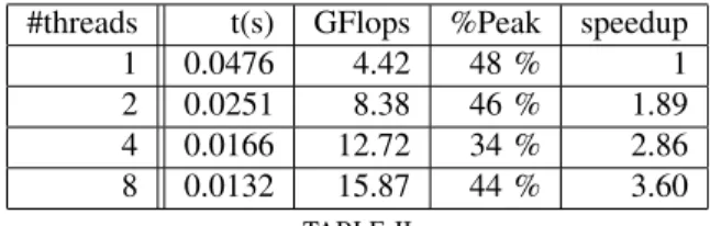
#threads t(s) GFlops %Peak speedup 1 0.0476 4.42 48 % 1 2 0.0251 8.38 46 % 1.89 4 0.0166 12.72 34 % 2.86 8 0.0132 15.87 44 % 3.60
TABLE II
PERFORMANCE OF THE POOL OF TASKS SCHEDULING
We observe an improvement of the scalability, thus a better overall performance. Table III shows the performances with various number of tasks in the pool ranging from 4 to 4096.
4 8 16 32 64 128 4 threads 9.78 9.47 11.24 12.37 12.51 12.72 8 threads 10.02 12.52 13.85 15.52 13.10 15.87 256 512 1024 2048 4096 -4 threads 12.20 12.29 11.76 12.45 13.26 -8 threads 16.99 13.52 16.25 15.80 8.33 -TABLE III
GFLOPS PERFORMANCE WITH VARIOUS POOL CARDINALITIES
We see that a pool of 128 tasks is the most suitable.
C. Scheduling for both Spinor and SU3 reuses
Spinors data dependencies are only between odd-even sites, and two consecutive sites with the same parity share one of their respective height dependent spinors. Thus, when computing the spinors of an odd (resp. even) sublattice in the lexicographical order of its sites, spinors reuse is granted because of this recurrent memory footprint intersection. This is why, even if there is a factor 8 data redundancy related to spinors use, the corresponding impact on the effective performance does not appear to be so offending.
The case of SU(3) matrices is different. First, each SU3 is used twice by a pair of two connected sites, thus the best reuse one could achieve is bounded by a factor 2. A strict application of the gauge copy storage completely drops any reuse expectation. Since the odd sublattice shares exactly the same set of SU3 matrices with the even sublattice, we suggest to keep the gauge copy for the odd sites and pick up the required SU(3) matrices for the even sites from their previous locations. So, we sacrifice data locality for data sharing or reuse. But this just a compromise as it applies only on the half set of sites. We will later see that this counterpart disappears with the way we organize the data for vector computing.
Putting together the previous two analyses including the asymmetric management of the SU(3), we suggest to alterna-tively iterateover the odd and the even sublattices in order to target the maximum cache sharing for both spinors and SU(3) matrices. Figure Fig. 1 depicts the scheduling for a binary lattice. Thus, the horizontal walk is for spinors reuse, while the vertical walk is for SU(3) matrices reuse.
Fig. 1. Alternating Even-Odd Scheduling
The results obtained with this approach are given in table Table IV, were each even-odd switch is performed after a small chunk of iterations rather than a single one as originally presented.
#threads t(s) GFlops %Peak speedup 1 0.0499 4.23 44 % 1 2 0.0257 8.21 43 % 1.98 4 0.0177 11.88 32 % 2.81 8 0.0126 16.71 40 % 3.96
TABLE IV
IMPACT OF THE EVEN-ODD ALTERNATING SCHEDULING
We see a slight improvement of both scalability and overall performance compared to the baseline. The most surprising here is that this irregular indexing of the SU(3) matrices for odd lattices is not so penalizing, this might be due to high-level caches sharing as expected. We think that this aspect needs more investigation, we leave it for future work. D. AoS to SoA Approach for Efficient Vectorization
AoS-SoA is a well-know data layout transformation aiming at creating regular data accesses depending on the target and the computation paradigm. Vector computing is an important candidate for this approach, since data to be processed should be prepared for vector accesses. In our case, considering double precision and 256-bit-wide vector registers, we just replace the original complex data type
typedef struct { double re, im; } complex; by
typedef struct { m256d re, im;} complex simd;
within the data structures associated to spinors and SU(3) matrices. Afterwards, we design and implement a vector version (using AVX intrinsics) of the linear algebra kernels. Now comes the explicit data shuffling that is required in order to have the vector operands ready for the compu-tation. For instance, if we consider four spinor structures s(j)= [s(j)
1 , s (j)
2 , · · · ], j = 1, 2, 3, 4, the corresponding vector
structure would be s = [s(1)1 s(2)1 s(3)1 s(4)1 , s(1)2 s(2)2 s(3)2 s(4)2 , · · · ]. The s(j) are not required to be consecutive in memory, thus one might expect a penalty from the extra memory cost due to this explicit packing. The stencil nature of LQCD computation exacerbates this fear. Since SU(3) matrices are constant, they are packed once before the computation, thus should not be really counted as an extra dynamic processing. For the spinors, there is no choice other than doing this on the fly. The experimental performance of our effort in that direction are reported in table Table V.
#threads t(s) GFlops %Peak speedup 1 0.0261 8.07 84 % 1 2 0.0144 14.68 76 % 1.82 4 0.0128 16.45 42 % 2.04 8 0.0140 15.03 39 % 1.86 TABLE V PERFORMANCE WITHAOS-TO-SOA
We see an important factor 2 improvement on a single core (and nearly the same on 2 cores), but a weak scaling beyond 2 cores. We now address this point by reducing the culprit
memory bandwidth and the expense of extra floating point operations.
E. Two-rows SU3 reconstruct
We recall that the third row of a SU(3) matrix can be reconstructed by taking the complex conjugate of the cross product of the first two rows (i.e. u3 = u1∧ u2). Thus,
our data structure for SU3 matrices does no longer include the third row, which is then reconstructed on the fly each time needed. This strategy saves some memory bandwidth and reduces cache pollution. The performance results on our working scenario are shown in table Table VI, the extra flops counting for the SU(3) reconstructs are not considered.
#threads t(s) GFlops %Peak speedup 1 0.0233 9.06 94 % 1 2 0.0139 15.12 79 % 1.67 4 0.0099 21.27 55 % 2.35 8 0.0094 22.38 58 % 2.47
TABLE VI
EFFECT OF THE TWO-ROWS RECONSTRUCT
We get an additional flops of 10% on a single core and 20% globally, with a relative improvement of 40% and a better scalability. This is also another evidence that the memory bandwidth associated to SU3 matrices is critical. We now move to the section devoted to our experimental results on the newly released INTEL-BROADWELL processor.
VII. EXPERIMENTALPERFORMANCEMEASUREMENTS
A. Platform Description
We consider the newly released INTEL-BROADWELL
-BASEDprocessor described in figure Fig. 2.
Fig. 2. INTEL-Broawell Main Specifications
Considering the available 256-bit-wide vector registers and the corresponding vector processing capability using AVX2, we obtain a peak performance of 2.2 × 4 = 8.8 GFlops/core in double precision, which might be higher with the Turbo Boost.
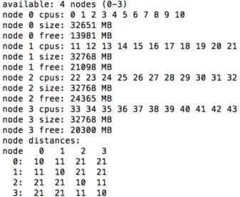
The numactl --hardware command gives the infor-mation displayed in figure Fig. 3.
Fig. 3. Numa Specifications of our Hardware
From this NUMA observation, we say that the appreciation of our experimental results should focus on the 11 cores of a single node, since our implementation at this stage is not explicitly numa-aware, with hyperthreading not activated at the time of our experimentations.
B. Experimental results on INTEL-BROADWELL
Table VII presents our experimental results up to 11 threads, where in each scenario, we bind the process to a single node for the previously explained reasons.
#threads t(s) GFlops Peak %Peak speedup 1 0.0300 7.02 8.8 80 % 1 2 0.0159 13.28 17.6 75 % 1.89 3 0.0115 18.31 26.4 69 % 2.61 4 0.0087 24.19 35.2 69 % 3.45 5 0.0072 29.41 44.0 67 % 4.19 6 0.0062 33.93 52.8 64 % 4.83 7 0.0056 37.58 61.6 61 % 5.35 8 0.0053 39.91 70.4 57 % 5.69 9 0.0050 42.06 79.2 53 % 6.00 10 0.0048 44.32 88.0 50 % 6.25 11 0.0044 48.02 96.8 50 % 6.81 TABLE VII
PERFORMANCE ON ONEINTEL-BROADWELL NODE
We see that the performances on one core is impressive and the absolute efficiency slowly decreases as the number of threads is increasing. We end up with 50% of the peak on a full node with its 11 cores. We need to stress the fact our computations are performed in double precision. In [9] for instance, where single precision is considered, a global performance of 250 GFlops is obtained on an Intel Xeon Phi 5110P, whose peak performance is 1.053 × 16 × 60 = 1010.88 GFlops in single precision, thus a sustained efficiency of 25%. As stated previously, most of authors consider single precision, as this reduces memory bandwidth and increases
the potential of vectorization, among other reasons. Showing good performances in double precision is thus one of the strength of this paper. However, some important points need more investigation, and others are worth considering too. We now describe a few of them.
VIII. FUTUREWORK
We point out some important aspects that we think should be investigated deeply. We plan to keep investigating most of them.
First, NUMA-awareness needs a serious attention. Indeed, the trend in the design of modern high-performance processors is to increase the number of cores, each of them with a moderate clock frequency. The packaging of the processor cores into different chips and different sockets, all of them sharing the same efficient but complex memory system, yields several NUMA nodes which should be skillfully addressed in order to seek an acceptable level of scalability. The case of LQCD, with the stencil nature of its computation, looks challenging.
Because of the threads scalability issue, among other rea-sons, the message passing paradigm seems to be widely considered, even with shared memory systems. Although this pragmatic approach is understandable in general, we think that hybrid approaches are worth considering. Indeed, even if message passing implementations can run as such on a shared memory node, explicit data exchanges have a significant cost and might trigger noisy synchronizations. For such exchanges, as long as all communicating processes reside on the same compute node, we are limited by the memory bandwidth available. Once more nodes become involved, the network bandwidth, usually much lower than the memory bandwidth, becomes the limiting factor. The case applications that expose heavy data exchanges like LQCD are particularly sensitive to this aspect, whose intensive experimental studies should also help to assess any technical guess.
As explained and illustrated in this paper, optimizing the memory traffic associated to SU(3) matrices would certainly yield a noticeable global performance improvement. Beside existing approaches like the gauge copy and the two-rows com-pression, other strategies should be examined. Our even-odd alternating scheduling, intended to bring some level of SU(3) reuse, is still providing a marginal effect at this stage, thus needs a deeper exploration. In addition, explicit prefetching mechanisms could be studied, at least at higher level caches.
Data exchanges in the context of distributed memory ma-chines is also of a central importance. Indeed, it is likely to consider large-scale computing clusters for LQCD simulations. Even when following the way to hybrid implementations, the number of communicating nodes remains important when considering large supercomputers, and the gap between the virtual topology (following the tasks graph) and the effective one (following the interconnect of the machine) is usually important and penalizing. Thus, in addition to considering a shared memory approach at the computing node level, studies
that address interprocessor communication in the perspective of better performances are of a keen interest.
IX. CONCLUSION
We have presented our view and efforts on the Wilson Dslash operator of LQCD. Considering the challenging double precision case, we have been able to get more than 50% of the overall peak on one 11-cores chip of the INTEL BROADWELL
based on Intel Xheon E5-2699 processors. Our initial efforts on a single core, considering AoS-to-SoA transformation fol-lowed by a fast corresponding AVX implementation, together with the two-rows gauge compression, yields a sustained performance beyond 80% of the peak. We think that, when it comes to large computing clusters, harvesting the potential of single node at the best, before moving to the message passing extension, will have a good impact on the overall performance. This is one of our ongoing work.
ACKNOWLEDGMENT
This work was initiated from the PetaQCD projet funded by a grant from ANR, the french national agency for research, through the program COSINUS. We also expresse our sincere gratitude to Philippe Thierry from INTEL to have provided us an access to their Broadwell-based machine.
REFERENCES [1] https://www.petaqcd.org/?lang=en
[2] D. Barthou, G. Grosdidier, M. Kruse, O. P`ene, and C. Tadonki, QIRAL: A High Level Language for Lattice QCD Code Generation, ETAPS 2012, Tallin - Estonia (2012)
[3] F. Belletti, G. Bilardi, M. Drochner, N. Eicker, Z. Fodor, D. Hierl, H. Kaldass, T. Lippert, T. Maurer, N. Meyer, A. Nobile, D. Pleiter, A. Schaefer, F. Schifano, H. Simma, S. Solbrig, T. Streuer, R. Tripiccione, and T. Wettig. QCD on the Cell Broadband Engine, Oct 2007. [4] Clark, M.A., Babich, R., Barros, K., Brower, R.C., Rebbi, C.: Solving
Lattice QCD systems of equations using mixed precision solvers on GPUs. Comput. Phys. Commun. 181 (2010) 15171528.
[5] R. G. Edwards, Balint J´o, and T. Jefferson, The Chroma Software System for Lattice QCD
http://arxiv.org/pdf/hep-lat/0409003.pdf [6] QDP++,
http://www.top500.org/system/177003.
[7] G.Grosdidier, Scaling stories, PetaQCD Final Review Meeting, Or-say,France, Sept. 27th 28th 2012.
[8] K. Z. Ibrahim and F. Bodin, Implementing Wilson-Dirac operator on the cell broadband engine, ICS ’08: Proceedings of the 22nd annual international conference on Supercomputing, pp. 4-14, Island of Kos, Greece, 2008.
[9] B. Jo´o, D. D. Kalamkar, K. Vaidyanathan, M. Smelyanskiy, K. Pamnany, V. W Lee, P. Dubey, and W. Watson, Lattice QCD on Intel Xeon Phi https://software.intel.com/sites/default/files
/article/401382/qcd-isc2013.pdf
[10] K. Jansen and C. Urbach, tmLQCD: a program suite to simulate Wilson Twisted mass Lattice QCD, Computer Physics Communications, vol. 180(12), p. 2717-2738, 2009.
[11] Y. Li, I. Pandis, R. Mueller, V. Raman, and G. Lohman, NUMA-aware algorithms: the case of data shuffling
http://www.pandis.net/resources/cidr13numashuffling.pdf 2013.
[12] R. Al-Omairy, G. Miranda, H. Ltaief, R. M. Badia, X. Martorell, J. Labarta, and D. Keyes, Dense Matrix Computations on NUMA Architec-tures with Distance-Aware Work Stealing, Upercomputing Frontiers and Innovations, vol. 2(1), 2015.
[13] M. Luscher, Implementation of the lattice Dirac operator, 2006. [14] D. Pleiter, QPACE: Power-efficient parallel architecture based on IBM
[15] QDP++,
http://usqcd.jlab.org/usqcd-docs/qdp++/.
[16] Smelyanskiy, M., Vaidyanathan, K., Choi, J., Joo, B., Chhugani, J., Clark, M.A., Dubey, P.: High-performance lattice QCD for multi-core based parallel systems using a cache-friendly hybrid threaded-MPI approach In: Proceedings of 2011 International Conference for High Performance Computing, Networking, Storage and Analysis. SC 11 (2011) 69:169:11
[17] C. Tadonki, G. Grosdidier, and O. Pene, An efficient CELL library for Lattice Quantum Chromodynamics, International Workshop on Highly Efficient Accelerators and Reconfigurable Technologies (HEART) in con-junction with the 24th ACM International Conference on Supercomputing (ICS), pp. 67-71, Epochal Tsukuba, Tsukuba, Japan, June 1-4, 2010. ACM SIGARCH Computer Architecture News, vol 38(4) 2011. [18] C. Urbach, K. Jansen, A. Shindler, and U. Wenger, HMC Algorithm with
Multiple Time Scale Integration and Mass Preconditioning, Computer Physics Communications, vol. 174, p. 87, 2006.
[19] C. Van Loan, Computational Framework for the Fast Fourier Transform, SIAM, 1992.
[20] P. Vranas, M. A. Blumrich, D. Chen, A. Gara, M. E. Giampapa, P. Heidelberger, V. Salapura, J. C. Sexton, R. Soltz, G. Bhanot, Massively parallel quantum chromodynamics, IBM J. RES. & DEV. VOL. 52 NO. 1/2 JANUARY/MARCH 2008.
[21] F. Wilczek, What QCD Tells Us About Nature and Why We Should Listen, Nuc. Phys. A 663, 320, 2000.