Meta-Models For The Assessment Of Soil Stochastic Properties From Monitoring: Application To Harbour Structures

HAL Id: hal-01008418

https://hal.archives-ouvertes.fr/hal-01008418

HAL is a multi-disciplinary open access archive for the deposit and dissemination of sci-entific research documents, whether they are pub-lished or not. The documents may come from teaching and research institutions in France or abroad, or from public or private research centers.

L’archive ouverte pluridisciplinaire HAL, est destinée au dépôt et à la diffusion de documents scientifiques de niveau recherche, publiés ou non, émanant des établissements d’enseignement et de recherche français ou étrangers, des laboratoires publics ou privés.

Meta-Models For The Assessment Of Soil Stochastic

Properties From Monitoring: Application To Harbour

Structures

Katheirne Le, Franck Schoefs, Francesca Lanata

To cite this version:

Katheirne Le, Franck Schoefs, Francesca Lanata. Meta-Models For The Assessment Of Soil Stochas-tic Properties From Monitoring: Application To Harbour Structures. 5th European Conference on Structural Control (EACS 2012), Jun 2012, Genoa, Italy. �hal-01008418�

1

*_{Corresponding author}

META-MODELS FOR THE ASSESSMENT OF SOIL STOCHASTIC

PROPERTIES FROM MONITORING: APPLICATION TO HARBOUR

STRUCTURES

K.T. LE, F. SCHOEFS & F. LANATA

LUNAM Université, University of Nantes-Centrale Nantes-CNRS, GeM, Institute for Research in Civil and Mechanical Engineering, UMR 6183, 2, rue de la Houssinière BP 92208 44322 Nantes Cedex 3, France

ABSTRACT

Since several decades, quite a lot of structures have been monitored to analyze their displacement during the works or during the service-life. Generally only deterministic measurements of some locations in the structure or the soil are considered. In some cases, we can get more information: When several sensors are placed in similar sections of the structure; when the loading is deterministic and the short term condition of the soil can be measured during this loading. In both cases the probabilistic characterization of soil parameters can be performed once both the structural model and measurements is considered as sufficiently accurate. The paper considers the monitoring of wharves for illustrating the behaviour of complex wharves when loading and soil parameters are random; here tie-rods are instrumented. The modelling is performed though a meta-model fitted on a numerical database obtained from direct simulations on a complex finite element model under Plaxis software: a quadratic Response Surface Model (RSM). This first contribution allows developing an inverse analysis and identifying soil characteristics.

Keywords: monitoring, wharves, soil variability, response surface methodology, inverse analysis.

1 INTRODUCTION

In the context of maintenance and new design of existent civil engineering structures, improvement of the in-service behaviour requires disposing of a wide range of technical and methodological tools allowing a decision support based on rational tools. Among these tools we can mention on the one hand, the data collection, concerning a feedback, and on the other hand, modelling of progressive phenomena such as fatigue and corrosion. Systematic predictive maintenance programs are not easy to implement in a whole system of infrastructures due to heterogeneity of building ages and building techniques. This is the case of structures in coastal area. The survey of structures (displacement) gives additional information but the updating of the modelling is a great challenge when a lot of influencing factors are involved. Thus, intrusive structural monitoring of complex structures is actually the only way on the one hand, for reaching as close as possible their real in-service behaviour, influenced by building conditions and settlements that are expected to separate the present behaviour from the theoretical one ([9;21;32]), and on the other hand to understand complex interaction mechanisms, as soil-structure interaction for example ([10;28]).

Due to the randomness of building (concrete, embankment) and natural properties of material (soil), probabilistic methods are more and more considered. They offer the theoretical framework to deal with uncertainties involved in structural assessment of Civil Engineering structures in view to perform sensitivity analysis or reliability assessment.

In this paper we focus on the characterization of powdery embankment physical and mechanical properties for soil pressure quantification. Moreover, we aim to characterize the randomness of characteristics of soil properties from the monitoring of tie-rods in a wharf. First a complete model of the wharf is suggested and a meta-model is suggested as a surrogate to this complex and time-consuming model. We present several polynomial response surfaces to this aim and samples are built in view to fit these meta-models on a data base with a probabilistic meaning. We finally identify the soil properties and focus the analysis on the frictional angle.

2 DESCRIPTION OF THE STRUCTURE, THE INSTRUMENTATION AND AVAILABLE DATA

2.1 Description of the structure

The studied structure is the extension of the timber terminal of Cheviré, the station 4, named Cheviré-4 wharf. The Cheviré-4 wharf is located downstream of the Cheviré bridge near Nantes city (west of France), in a river environment, on the left strand of the river Loire. It is 180 m long and 34.50 m wide. Collaboration with the Port Authority of Nantes Saint-Nazaire (PANSN) permitted the survey of the structure. A sketch of a typical cross section and main components is presented on Fig. 1. Each component plays a specific role in the functioning of the pile-supported wharf in a functional context.

Fig. 1. Cross section of the wharf

2.2 Structural instrumentation

Instrumentation strategy aims following the global behaviour of the wharf during at least 5 years after building with a view to improve prediction models. These validated models will allow basing the maintenance policy on a better understanding of the in-service behaviour. Indeed, the large dimensions of these structures, the building hazards and the soil behaviour imply the service behaviour is very different from the expected design one induced by the choice of conservative and too theoretical hypotheses at the design stage.

The objective being the understanding of the wharf behaviour under horizontal loading − actions of the embankment, ship berthing and wind action on the cranes −, we chose to monitor the tie-rods, which are sensitive elements of the wharf that are not accessible after the building period. The wharf has been instrumented on twelve tie-rods (regularly distributed along the length of the

wharf, see Fig. 2) in order to follow the normal load in the rods cross-section. Electric strain gauges have been used, mounted in full bridge and bonded to the rods with a high temperature epoxy resin used for sensors manufacturing; these gauges are linked to a “Campbell Scientific CR10X” data logger. The wiring of strain gauges in a full bridge ensures a temperature self-compensation. The system also ensures the corrosion protection of the rods. A tidal gauge (controlled by PANSN) measures the real tide level every 5 minutes; this tidal gauge is located 1 km downstream the Cheviré bridge. The interest of these measurements is that the over-crests, due to the air pressure, the rate of the river flow and the wind, are taken into account.

Fig. 2. View of the instrumentation plan

2.3 Available data

Measured loads in the tie-rods come from a two years monitoring period (from January 2004 to October 2005) and have been analyzed in [33]. Two types of variations characterize the loads in the tie-rods:

- temporal: medium-term variations, where the levels of loads are questioned during a month (about a period of the moon rotation) and short-term variations where the interest is in the amplitude of the loads during a tide with a period of about 12 h;

- spatial: variations of the load in each spatially distributed tie-rod.

The analysis of the spatial load variations shows an important scatter from a tie-rod to another. These variations have been analyzed in [33]. Yáñez-Godoy et al. have shown that when considering the variation of this loading during a tide, it is much more stable from a tie-rod to another one and in time. This paper focuses on this behaviour.

2.4 Main assumptions for probabilistic modelling from spatial profile and time-series

Since a decade, investigations of structural behaviour through Non Destructive Testing or Monitoring have underlined the need for methods of data processing and structural computation. We classify the obtained time-series in three categories:

- time-series describing the evolution of an ageing phenomena like chloride ingress in concrete, crack propagation,

- time-series measuring the strain affected by non-periodic loading like wind and truck loading,

- time-series measuring the strain due to cyclic loading like temperature, tide or waves.

This paper focuses on data obtained from the two last categories during the training period that means before any ageing mechanism occurs. Moreover, when similar components placed at a given location xi are monitored (beams [17] or tie-rods [33]), and subjected to the same loading, a statistical study of their loading LT(xi, t, θj ) can be performed, where t denotes the time and θj the event that represents mainly the hazard during building works and composition of the material

around; θj is a realization of the hazard θ, θ∈ Ω, the probabilistic space that gather all the hazard that generates events, thus realization of random variables (material properties, tide level, …). Finally, if we consider components in the soil (sheet-piles, piles, rods), cyclic variation of the water level modify its granular structure with time i.e. the composition of the material. Thus, each loading at time t can be considered as the loading on the same component in other material conditions. With this assumption and an abuse of notation, LT(xi, t, θj ) is replaced by LT(xi, θk ). Moreover the paper focuses on the loading during tidal variations and in that case the spatial variation cannot be proved [33], thus LT (xi, θk) is replaced by LT(θk ). Fig. 3 represents the evolution of the sensitivity of the loading during a tide with time (number of the week in 2004) for a given tie-rod (R0) and three coefficients CMAR (42, 69, 100): in France, the oscillation amplitude of semi-diurnal tide is associated to a coefficient named tide coefficient CMAR (see [33] for the definition). We observe that the scatter is high for CMAR=42. Phenomena seem to be more complex at lower CMAR. In this paper, we aim to provide a probabilistic model of soil properties for reliability analysis of wharf during storms [34]. These extreme events occur mainly in winter when CMAR are higher. In the following, we analyze only the horizontal wharf behaviour for these conditions.

Fig. 3. Variation of the measured normal load ΔF in the tie-rod R0 in relation to water level

variation of the river Loire ΔH for a falling tide (CMAR: 42, 69, 100)

3 NUMERICAL MODELLING AND META-MODEL ASSESSMENT 3.1 Numerical strategy

Numerical models must be integrated in the future in an optimization procedure in view to identify the soil characteristics. Computation time should be reduced as low as possible due to the necessary huge number of calls to the model for optimization procedures. Thus we suggest to develop a complete two-dimensional Finite Element Model (FEM) under the PLAXIS environment [8] and to find the best meta-model M(X(θj)) –with X(θj) input random variables- to represent this numerical behavior. The choice of PLAXIS is governed by the fact that the interface of this software allows implementing the phases of the real works and offers a wide set of soil properties and behaviour. It is well recognized to reach a realistic behaviour of geotechnical structures. Several meta-models have been developed for deterministic or probabilistic analysis of wharves during these two last decades: neuronal and Bayesian networks ([24;25]), spectral stochastic finite element models based on regression or projection methods ([4;26]), polynomial or other response surfaces.

We decide here to select quadratic polynomial response surfaces due to their asymptotic properties ([1;5;19;25]).

3.2 Finite Element Model

The problem is modeled through a PLAXIS finite element model by considering all the work phases. Fig. 4 depicts the geometry and the several level of soil. We use a 2-D model to represent a standard cross section, not affected by the ends and consistent with the assumptions in 2.4. At 3 meters deep under the embankment surface is installed a barbican (drainage channel) in view to reduce the water pressure on the wharf when the falling tide. Moreover, due to the presence of the sheet-pile, the effect of the flow in the soil under the screen is neglected. The main characteristics of the mechanical model are gathered in Table 1 (see [26] for details). Note that the backwharf wall has a L-shape and is composed with two plates (Fig. 4).

Table 1 – Main structural characteristics.

Structural component Mechanical Behaviour EA

(kN/m) EI (kNm2/m) γ (kN/ml/m) ν E (kN/m2)

Spring (platform + piles) Linear elastic 20.91*103

Plate (backwharf wall) Linear elastic EA1=3.08*10

4 EA2=1.4*104 EI1=410.7 EI2=746.7 γ1=22,8 γ2=20,8 0.1 35000

Tie-rod Linear elastic 971437

Geogrid (c-anchoring plate) Linear elastic 105

Sheetpiles Linear elastic 3.32*106 6.45*104 1.245 0.1 210*106

γ denotes the weight per linear meter of wharf (ml) per meter of depth

We have tested several models for the limit conditions of the anchoring plate at one end of the tie rod: plate or geogrid. The best model that follows the tide loading with time was the geogrid. For the same reason, the connexion between the backwharf wall and the sheet pile is a hinge. Schoefs et al. [26] have shown that the concrete platform and the piles can be modelled by an embedded horizontal beam with deterministic behaviour (see Fig. 4); the rigidity of the platform in the horizontal plane reduce the variance of each pile connected to it and is much larger than tie-rod axial rigidity.

Fig. 4. Geometry modelled under PLAXIS environment by the FE model.

During a tide, the water level varies both in the embankment and the river. We consider 6 phases for the description of these phases. Fig. 5 illustrates two phases (1 and 6) obtained for a tide coefficient CMAR=69.

EA1

Fig. 5. Water levels in embankment and river on phase 1 (left) and 6 (right)

3.3 Meta model: Quadratic Response Surfaces

Nowadays, quite a lot of response surface functions have been tested in several areas. We generally distinguish two types of models ([1;25]): the physical response function and the analytical response function. We focus here on the second one and more especially on the polynomial models of order less than 3 with or without interaction terms, called Quadratic Response Surfaces (QRS) and developed in several fields ([7;11;12;22]). This form has specific properties especially an asymptotic behaviour for the transfer of distribution tails that fits the physical meaning. It is essential when only few experiments are available to ensure a realistic transfer of distribution tails ([15;19]).

The general form of the full QRS is the following:

∑

∑

∑

where LT,SR is the load in the tie-rod, Xi is the ith random variable and the bk values are determined by regression method from a numerical experimental plan based both on the probabilistic distribution of the variables (distribution of numerical values) and their potential influence on the response (number of numerical values –i.e. size of the sample - for each variable).

By putting various coefficients equal to zero, various several mathematical models were formed, compared to experimental data, and the coefficients determined by response surface function:

- Pure quadratic if bi = 0 and bij,i≠j = 0; - Linear with interaction if bii = 0; - Linear if bij,i≠j = 0 and bii = 0;

The more complex is the model the more data are needed to identify coefficients.

4 RANDOM VARIABLES AND PROBABILISTIC MODELING 4.1 Numerical experimental design

For identifying values of coefficients bk in (1), we fit a QRS on a numerical database with a probabilistic sense: that means that samples are generated from a probability density function for each variable. Basic random variables selected herein are: γsat and γunsat respectively saturated and unsaturated own-weight of the embankment, E and ν its respective Young and Poisson modulus and

φ its internal frictional angle. Cohesion c is neglected.

The range of variation for each variable is selected from literature or preliminary knowledge. Table 2 summarizes the selected basic variables, their distribution, parameters (range if bounded) of the distributions and selected values for experimental design. Note that we selected uniform distribution for soil parameters due to the lack of previous knowledge: with this type of distribution,

a large weight is affected to values on distribution tails. A deterministic functional relationship is used between unsaturated γunsat and saturated γsat own weight of the embankment to reduce the number of independent variables: γsat = γunsat + 2. Concerning the tide-river level and the corresponding level of water in the embankment, we consider a tide with a high and frequent CMAR of 70. In the two years database, a CMAR of 69 has been observed: the 2nd of March 2005 with a high level Hmax = 6.21m and a low level Hmin = 2.19m from the 0 level of the sea along the French coasts. Fig. 6 depicts the distribution of the tide-river levels measured during the two years and we can observed that Hmax and Hmin are representative of mean values for each distribution. We choose to discretize the tide-river lever in six phases (see Table 3) between these values to get a good representation of potential situations during this type of tide (see Fig. 4 for phases 1 and 6). They can be also seen as other extreme tide levels. For each of this water level, a water level in the embankment has been measured. From this experimental design and basic variables assumed to be independent, a total amount of 450 computations were performed with Plaxis Finite Element model.

Table 2 – Pre-selection of variables and distributions.

Variables Distribition Size of the support/parameters Selected values for simulation

Own weight (kN/m3) γsat Relationship with γunsat

γunsat Uniform [16÷20] 16, 17, 18, 19, 20

Young modulus E (Mpa) Uniform [30÷50] 30, 35, 40, 45, 50

Frictional internal angle φ (°) Uniform [25÷35] 25, 27, 30, 32, 35 / 25 30 35

Poisson modulus ν (-) Uniform [0.25÷0.4] 0.25, 0.3, 0.35, 0.4 / 0.27

Cohesion c (kPa) Determinsitic 0

High tide level Hmax Generalized Exterme value µ= 5.84; σ= 0.69 See Table 3

Low tide level Hmin Generalized Exterme value µ= 1.61; σ=0.79 See Table 3

In bold characters: used for QRS calibration (section 4.3).

-1 0 1 2 3 4 5 6 7 0 0.1 0.2 0.3 0.4 0.5 0.6 0.7 0.8 0.9

Water level of Loire (m)

De

n

s

it

y

Max and min tide distributions

Data_hmax PDF_hmax Data_hmin

PDF_hmin

Figure 6. Water levels of the tide measures during the two years

Sand characteristics are considered as deterministic because they play a lesser role on the horizontal behaviour: γunsat =19 kN/m3; E = 30 MPa; φ = 30 (°) ; ν = 0.001; dilatancy angle ψ = 0.

Table 3 – Selected phases of water level during a tide CMAR=69

Phases Tide-River level (m) Water level in embankment (m)

Phase 1 6.21 5.19 Phase 2 5.75 5.39 Phase 3 4.84 5.19 Phase 4 4.17 4.96 Phase 5 2.98 4.54 Phase 6 2.19 4.13

4.2 Uncertain and sensitivity analysis

With the 6 random variables presented in Table 2, 28 coefficients should be calibrated to fit a full quadratic response surface. That leads to a huger database than the previous one. We use the first numerical database described above to highlight the most influent random variables and to reduce their number. All the results are available in [18]. They highlight the following key points: (i) 1/E and γunsat act in very similar way in the response (Fig. 7 for the two phases of Fig. 5); (ii) ν has no influence in the response.

Figure 7. Influence of own weight (left) and Young modul (right) in the response

Table 4 gathers the results and the conclusion concerning the selected Basic Random Variables (BRV). Four random variables are finally selected that leads to the calibration of 15 coefficients for a full quadratic response surface.

Table 4- Selection of input random for the calibration for response surface

Initial random variables Studies Relationship Name of selected BRV

γunsat : Unsaturated own weight Variable change

E

X_{1 =} γunsat _{[X1]: RV}

E : Young modulus Variable change

ϕ : Internal frictional angle - X2 = ϕ [X2]: BRV

γsat : Saturated own weight Functional relationship with γunsat

γsat = f(γunsat)

ou γsat = γunsat + ε

ν : Coefficient de Poisson Sensitivity analysis ν = 0.27 ν : deterministic parameter

Tide level of Loire Mesured data of CMAR69 - [X3]: BRV

Underground in the embankment Mesured data of CMAR69 - [X4]: BRV

4.3 QRS calibration and selection

Table 5 presents values of residuals obtained for the four quadratic response surfaces described in section 3.3 and from several criteria: the mean residual R (2); the mean relative deviation of residual ΔrF (3); and the likelihood of the parameters in the range [-10 kN;+10 kN]: this range correspond to the uncertainty in the measurement of loads themselves.

∑

∑

where Ri and FPli denote respectively the ith residual and value among N numerical experimentations.Here N = 450.

Table 5. Residuals values criteria for each type of RS

Criteria Linear Linear with Interaction Pure Quadratic Full Quadratic

Residuals (2) 0,732 0,566 0,574 0,343

Residuals (3) 0.067 0.049 0.051 0.031

Likelihood 0.48 0.59 0.58 0.83

The full quadratic response surface gives the best fitting. This is illustrated in figure 8 where we drawn the results of simulations obtained from Plaxis model and Linear and Full Quadratic response surfaces according to X1 and for three values of X2.

3 3.5 4 4.5 5 5.5 6 6.5 7 x 10-4 150 200 250 300 350 400 X1 = γ/E L O AD IN G I N T H E T IE-R O D (k N )

FULL QUADRATIC MODEL-PLAXIS

Fsr-(φ=25°) Fsr-(φ=30°) Fsr-(φ=35°) Fpl (+,x,*) 3 3.5 4 4.5 5 5.5 6 6.5 7 x 10-4 150 200 250 300 350 400 X1 = γ/E L O AD IN G I N T H E T IE-R O D (k N ) LINEAR MODEL-PLAXIS Fsr-(φ=25°) Fsr-(φ=30°) Fsr-(φ=35°) Fpl (+,x,*)

Figure 8. Plaxis simulations and response of full quadratic model (left) and linear model (right)

5 IDENTIFICATION OF BASIC RANDOM VARIABLES 5.1 Identification methodology

Levels of water in the river and in the embankment being monitored, X3 and X4 are known and identification procedure focuses on X1 and X2 only. We use a zero-order method (simplex) [16] based on the least square method for the identification of theses quantities for each tie-rod : one realisation is computed from the data of all the phases (29 phases) with 5 times of rising and falling during a tide of CMAR=69.

The cost function Ferr(θ) for the identification method is written as follows:

(

)

(

)

_∑

∑

∑

F , denotes the deviation between the ith measured load (

i

mes

F ) and the corresponding loading calculated by the numerical model of QRS (

i

sr

F ); ri(θ), denotes the deviation between measured loadings ith (

i

mes

F ) and the corresponding prediction f(Fsri,θ) by model of QRS; θ is unknown parameters that are identified.

10 i i 0 sr sr , ) F F F ( f θ = + (5)

where F0 is a quantity considered as part of the pre-loading during the installation of tie-rod and

Fsri is the loading in the tie-rod calculated by QRS. The value of F0 depends on each tie-rod due to its initial condition and it is calculated in the identification process of the variables.

The first interesting result is that we highlight the existence of two groups of tie-rods. The reason is still currently under discussion and should be found in the building method. Fig. 9 gives realizations of X1 and X2 for these two groups. No specific algorithm was used for distinguishing them because it appears clearly from the two separate clouds of points. That is why distinguish the fitting of probabily density functions (pdf) in two separate cases in the following.

0 0.2 0.4 0.6 0.8 1 1.2 x 10-3 36 37 38 39 40 41 42 43 44 X1 (γ/E) X2 ( φ ( °) )

DISTRIBUTION OF X1 AND X2, CMAR69

T4 T11 T17 T21 T31 T34

Figure 9. Distributions of X1 and X2 for the two groups

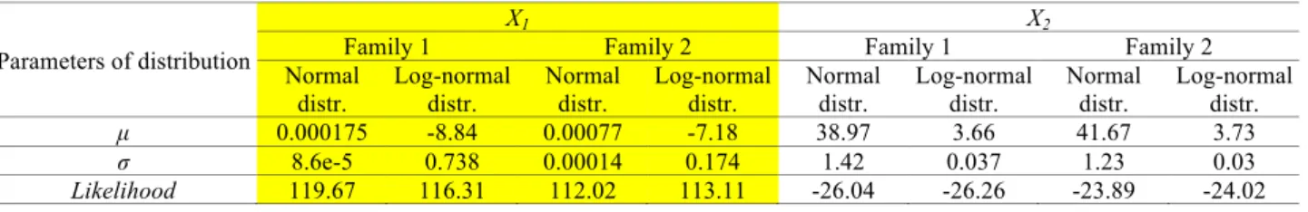
The correlation between two variables is considered by calculating the correlation coefficients between X1 and X2 for two families of tierods. These coefficients are respectively 0.1252 and -0.423 for families 1 and 2. They are low, this result allows us to formulate an assumption of independent random variables. We present the results of X2 only here. From Fig. 10 it is shown that the distribution can be well fitted by normal or log-normal pdf and that the support of the distributions contains acceptable values in comparison to litterature, the scatter being not too large (Table 6).

Table 6. Parameters of distributions of X1 and X2

Parameters of distribution

X1 X2

Family 1 Family 2 Family 1 Family 2

Normal distr. Log-normal distr. Normal distr. Log-normal distr. Normal distr. Log-normal distr. Normal distr. Log-normal distr. µ 0.000175 -8.84 0.00077 -7.18 38.97 3.66 41.67 3.73 σ 8.6e-5 0.738 0.00014 0.174 1.42 0.037 1.23 0.03 Likelihood 119.67 116.31 112.02 113.11 -26.04 -26.26 -23.89 -24.02 Group 2 Group 1

11 36 36.5 37 37.5 38 38.5 39 39.5 40 40.5 41 0 0.05 0.1 0.15 0.2 0.25 0.3 X2=φ (°) PD F

DISTRIBUTION OF X2-FAMILY 1, CMAR69 Donnée X2 Distr. normale Distr. lognormale 39 39.5 40 40.5 41 41.5 42 42.5 43 43.5 44 0 0.05 0.1 0.15 0.2 0.25 0.3 X2=φ (°) PD F

DISTRIBUTION OF X2, FAMILY 2, CMAR69 Donnée X2

Distr. normale Distr. lognormale

Figure 10. Distribution of X2, family 1 (left) and 2 (right)

5.2 Verification and validation

Let us now verify and validate the results from direct Monte-Carlo simulations using the fitted distributions above. Two periods of the tide are considered to analyze the accuracy of the response surface model. Fig. 11 left allows us to verify, here for tie-rod #4, that the model fits very well the measured loads: the measurements are very closed to the mean value and stay in the range of 5%-95% fractile of the output distribution of the model. Fig. 11 right gives the same plot for the same tie-rod but with another tide (CMAR=89). The plot shows a very good agreement between measurements and model: the measurements stay always in the range of 5%-95% fractile of the output distribution of the model.

0 5 10 15 20 25 30 310 320 330 340 350 360 370 380 390 400 410

Phases of tide (CMAR 69)

Loadi

ng

(k

N

)

LOADING IN THE TIE6ROD T4, NORMAL DISTRIBUTION OF PARAMETERS

Fmoy. Fmoy.5% Fmoy.95% Fmesuré 0 5 10 15 20 25 30 35 230 240 250 260 270 280 290 300 310 320 330

Phases of tide (CMAR 89)

Loadi

ng

(k

N

)

LOADING IN THE TIE-ROD T4, NORMAL DISTRIBUTION OF PARAMETERS

Fmoy. Fmoy.5% Fmoy.95% Fmesure

Fig. 11. Evolution of measured and modeled loading with time for T4 of CMAR=69 (left) and 89 (right)

6 CONCLUSION

Monitoring of infrastructures is currently used for damage detection. This paper focuses on another challenge: the identification of model characteristics from measured data. The application concerns geotechnical parameters of an embankment of a wharf. Due to intrinsic uncertainties on model and hazard on physical parameters, a probabilistic modeling is suggested. The question is first to provide a surrogate to the original model, here a quadratic response surface, and second a numerical database for the calibration. Here the full quadratic response surface is shown to be the most efficient to fit the finite element model. A reduction of the number of random variables is suggested and the model is used to identify distributions of parameters. Two groups of tie-rods are

12

then identified and the corresponding empirical distributions are provided. It is shown that both normal and log-normal pdf are convenient for the fitting of frictional angle. Verification and validation of the response surface model show that both the QRS and the distribution of identified parameters are convenient for a reliability analysis.

7 AKNOWLEGMENTS

This work is supported by nantes harbour and the European Community and FEDER founds within the duratiNet Interreg (Atlantic space, project N° N°2008-1/049) (duratiNet: Durable Transport Infrastructures in the Atlantic Area).

REFERENCES

[1] Baroth J., Breysse D., Schoefs F. (coord). 2011, Construction reliability, ISTE Ltd - Wiley, 368p.

[2] Bergado D., T. Youwai S., Teerawattanasuk C., Visudmedanukul S., 2003. « The interaction mechanism and behavior hexagonal wire mesh reinforced embankment with silty sand backfill on soft clay”. Computers and Geotechnics, vol. 30(6), 517-534.

[3] Boéro J. 2010. Fiabilité des infrastructures portuaires : Approche innovante d’analyse et de modélisation probabiliste des données d’inspection. PhD Thesis. Thèse sciences l’ingénieur Génie Civil et mécanique. Université de Nantes-UFR Sciences et techniques, Ecole doctorale « Sciences pour ingénieur, Géosciences, Architecture ».

[4] Boéro J., Schoefs F., Yáñez-Godoy H., Capra B., 2012, “Time-function reliability of harbour infrastructures from stochastic modelling of corrosion”, European Journal of Environmental

and Civil Engineering, in press.

[5] Borges J.L., 2004. “Three dimensional analysis of embankment on soft soils incorborating vertical drains by finite element method”. Computers and Geotechnics, vol. 31(8), 665-676. [6] Borges J.L., Cardoso A.S., 2001. “Structural behavior and parametric study of reinforced

embankment on soft clays”. Computers and Geotechnics, vol. 28(3), 209-293.

[7] Bouyssy V., Rackwitz R. 1994, “Approximation of Non-normal Responses for Drag Dominated Offshore Structures”. Reliability and Optimization of Structural Systems. proc. 6 th, IFIP WG

7.5, Chapman and Hall, 1994, pp. 161-168.

[8] Chang K.T., Sture S., 1997. “Microplane modelling of sand behavior under non-proportional loading”. Computers and Geotechnics, vol. 21(3), 183-216.

[9] Del Grosso A., 2000, “Monitoring of infrastructures in the marine environment”, Int. Workshop

on Structural Control for Civil and Infrastructure Engineering. Communication.

[10] Donahue M. J., Dickenson S. E., Miller T. H., Yim S. C., 2005, “Implications of the Observed Seismic Performance of a Pile Supported Wharf for Numerical Modeling”, Earthquake Spectra, EERI, Vol. 21, No. 3, pp. 617-634, August 2005.

[11] Faravelli L. 1989, “Response Surface Approach for Reliability Analysis”. Journal of

Engineering Mechanics (ASCE), 115(12), 1989, pp. 2763-2781.

[12] Faravelli L. 1992, “Structural Reliability via Response Surface, in N. Bellomo and F. Casciati (Ed.)”, Proceedings of Iutam Symposium on Nonlinear Stochastic Mechanics, Springler-Verlag, 1992, pp. 213-223.

[13] Hinchberger S.D., Rowe K.R., 2003. “Geosynthetic reinforced embankment on soft clay foundations: predicting reinforcement trains at failure”. Geotextiles and Geomembrances, vol. 21(3),151-175.

13

[14] Jie Huang, Jie Han. 2010. “Two-dimensional parametric study of geosynthetic reinforced colum-supported embankment by coupled hydraulic and mechanical modeling”. Computers and

Geotechnics, vol. 3796), 638-648.

[15] Labeyrie J., 1997, “Response Surface Methodology in Structural Reliability”. Probabilistic

Methods for Structural Design, C. Guedes Soares (Ed.), Solid Mechnics ans its Applications,

Vol. 56, Kluwer Academic Publishers, pp. 39-58.

[16] Lagarias J.C., Reeds J.A., Wright M.H., Wright P.E., 1998. “Convergence Properties of the Nelder-Mead Simplex Method in Low Dimensions”. SIAM Journal of Optimization, vol. 9, no. 1, pp. 112-147.

[17] Lanata F., Schoefs F., 2012, “Multi-algorithm approach for identification of structural behaviour of complex structures under cyclic environmental loading”. Journal Structural

Health Monitoring, Published online before print February 22th 2011, Volume 11, No 1/January

2012, pp. 51-67, doi: 10.1177/1475921710397711.

[18] Le K.T (2012). Identification des caractéristiques aléatoires de remblais à partir du suivi de santé des structures : application aux structures portuaires. PhD Thesis.

[19] Leira B.J., Holmås T., Ferfjord K., 2003, “Response Surface Parametrization for Estimation of Fatigue Damage and Extreme Response of Marine Structures”, 9th Int. Conf. on Application of

Statistics and Probability in Civil Engineering, (ICASP9), Vol. 1, Theme E "Damage and

Deterioration", 2003 Millpress Rotterdam, pp. 589 - 598.

[20] Martel S., 2005. Etude expérimental et méthologique sur le comportement des écrans de soutènement. PhD Thesis. Thèse géotechnique de docteur de l’école nationale des ponts et chaussées.

[21] Martin N.J., Bell S.I., 1999, “The Restoration of Shuaiba Oil Pier, Kuwait”. Int. Conf. on

Monitoring and Control of Marine and Harbour Structures. Communication.

[22] Muzeau J.-P., Lemaire M., Besse P. et Locci J.-M. 1993, “Evaluation of reliability in case of complex mechanical behavior”. In Proc. OMAE, editor, Safety and Reliability, volume II, pages 47–56, 1993.

[23] PLAXIS, (2003), Reference manual, Version 8.

[24] Rechea C., Levasseur S., Finno R., 2008. “Inverse analysis techniques for parameter identification in simulation of excavation support systems”. Computers and Geotechnics, vol. 35, 331-345.XX.

[25] Schoefs F., 2008, “Sensitivity approach for modeling the environmental loading of marine structures through a matrix response surface”, Reliability Engineering and System Safety, Available online 19 June 2007, Vol. 93, Issue 7, July 2008, pp. 1004-1017, doi: dx.doi.org/10.1016/j.ress.2007.05.006.

[26] Schoefs F., Yáñez-Godoy H., Lanata F., 2011, “Polynomial Chaos Representation for Identification of Mechanical Characteristics of Instrumented Structures: Application to a Pile Supported Wharf”, Computer Aided Civil And Infrastructure Engineering, spec. Issue “Structural Health Monitoring”, First published online 2nd November 2010, Volume 26, Issue 3, pages 173–189, April 2011, doi: 10.1111/j.1467-8667.2010.00683.x.

[27] Sharma J.S., Bolton M.D., (2001). “Centrifugal and numerical modelling of reinforced embankment on soft clay installer with wick drain”. Geotextiles and Geomembrances, vol. 19(1), 164-174.

[28] Sundaravadivelu R., Gopala Krishna M., Chellappan V., 1999, “Monitoring the Behaviour of Diaphragm Walls of a Dry Dock”, Int. Conf. on Monitoring and Control of Marine and Harbour Structures. Communication; 1999.

[29] Takahaskhi A., Takemura J., 2005. “Liquefaction-induced large dispacement of pile-supported wharf”. Soil dynamics and Earthquake Engineering, vol. 25(11), 811-825.

14

[30] Tanchaisawat T., Bergado D.T., Voottipruex P., 2008. “Numerical simulation and sensitivity analyses of full-scale test embankment with reinforced lightweight geomaterials on soft Bangkok clay”. Geotextiles and Geomembrances, vol. 26(6), 498-511.

[31] Tandjiria V., Low B.K., The C.I., (2002). “Effect of reinforcement force distribution on stability of embankment”. Geotextiles and Geomembrances, vol. 20(6), 423-443.

[32] Vallone M., Giammarinaro S., 2007, “Monitoring of Termini Imerese harbour (Sicily, Italy) using satellite DInSAR data”, Applied Geophysics for Engineering. Communication.

[33] Yáñez-Godoy H., Schoefs F., Casari P., 2008, “Statistical Analysis of the Effects of Building Conditions on the Initial Loadings of On-piles Quays”. Journal Structural Health Monitoring 2008; 7-3: 245-63.

[34] Yáñez-Godoy H., Schoefs F., Nouy A., Casari P., 2006. “Extreme storm loading on in-service wharf structures: interest of monitoring for reliability updating”. Revue Européenne de Génie

Civil; 5-10:565-81.

[35] Youssef M.A., Levasseur S., Asouli A., Finno R., Malecot Y., (2010). “Comparison of two inverse analysis techniques for learning deep excavation response”. Computers and