Fundamentals of manipulator stiffness modeling using matrix structural analysis

HAL Id: hal-01984946

https://hal.archives-ouvertes.fr/hal-01984946

Submitted on 7 Aug 2019

HAL is a multi-disciplinary open access

archive for the deposit and dissemination of

sci-entific research documents, whether they are

pub-lished or not. The documents may come from

teaching and research institutions in France or

abroad, or from public or private research centers.

L’archive ouverte pluridisciplinaire HAL, est

destinée au dépôt et à la diffusion de documents

scientifiques de niveau recherche, publiés ou non,

émanant des établissements d’enseignement et de

recherche français ou étrangers, des laboratoires

publics ou privés.

matrix structural analysis

Alexandr Klimchik, Anatol Pashkevich, Damien Chablat

To cite this version:

Alexandr Klimchik, Anatol Pashkevich, Damien Chablat. Fundamentals of manipulator stiffness

modeling using matrix structural analysis. Mechanism and Machine Theory, Elsevier, 2018, 133,

pp.365-394. �10.1016/j.mechmachtheory.2018.11.023�. �hal-01984946�

Fundamentals of manipulator stiffness modeling using matrix structural analysis

Fundamentals of manipulator stiffness modeling

using matrix structural analysis

Alexandr Klimchik

,

Anatol Pashkevich

, Damien Chablat

c _{Laboratoire des Sciences du Numérique de Nantes (LS2N), UMR CNRS 6004, 1 rue de la Noe, 44321 Nantes, France} d _{Centre National de la Recherche Scientifique (CNRS), France}

Abstract

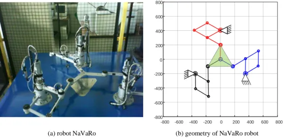
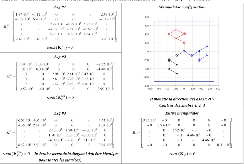
The paper generalizes existing contributions to the stiffness modeling of robotic manipulators using Matrix Structural Analysis. It presents a unified and systematic approach that is suitable for serial, parallel and hybrid architectures containing closed-loops, flexible links, and rigid connections, passive and elastic joints, flexible and rigid platforms, taking into account external loadings and preloadings. The proposed approach can be applied to both under-constrained, fully-constrained and over-constrained manipulators in generic and singular configurations, it is able to produce either non-singular or rank-deficient Cartesian stiffness matrices in a semi-analytical manner. It is based on a unified mathematical formulation that presents the manipulator stiffness model as a set of two groups of matrix equations describing elasticity of separate links and connections between the links in the form of constraints. Its principal advantage is the simplicity of the model generation that includes straightforward aggregation of link/joint equations without conventional merging of rows and columns in the global stiffness matrix. The advantages of this method and its application are illustrated by an example that deals with the stiffness analysis of NaVaRo parallel manipulator. Keywords:

Manipulator stiffness modeling, Matrix Structural Analysis, Cartesian stiffness matrix, Hybrid architectures, Passive joints

1

Introduction

In many modern robotic applications, manipulators are subject to essential external loadings that affect the positioning accuracy and provoke non-negligible positioning errors caused by the compliance of mechanical components [1, 2]. For this reason, manipulator stiffness analysis becomes one of the most important issues in the design of robot mechanics and control algorithms. It allows the designer to achieve required balance between the dynamics and accuracy since the usual reduction of manipulator moving masses or cross-sections leads to increasing of achievable speed and acceleration but also deteriorating undesirable compliance errors. However, to make the stiffness analysis efficient, it should rely on a simple and computationally reasonable method that is able to deal with complex architectures including numerous closed-loops, flexible links, rigid connections, passive and elastic joints that are common for hybrid robots.

At present, there exist three main techniques in this area, that are Finite Element Analysis (FEA), Matrix Structural Analysis (MSA) and Virtual Joint Modeling (VJM) [3-6]. The most accurate of them is the FEA [7-9], which allows modeling links and joints with their true dimension and shape. However, this technique is usually applied at the final design stage because of the high computational expenses required for high order matrix inversion [10, 11]. In contrast, the VJM method is treated as the simplest one, it is based on the extension of the traditional rigid model by adding the virtual joints (localized springs), which describe the elastic deformations of the links, joints and actuators [12-15]. This technique is widely used for serial and strictly parallel robots, but it can be hardly applied to the manipulators with more complex topology. The MSA is considered as a compromise technique, which incorporates the main ideas of the FEA, but operates with rather large elements such as flexible links connected by the actuated and passive joints in the overall manipulator structure [16-18]. This obviously leads to the reduction of the computational expenses that are quite acceptable for robotics, but it requires some non-trivial actions for including of passive and elastic joints in the related mathematical model. From the other side, the MSA is very convenient for a description of complex structures with numerous closed-loops and cross-linkage. For this reason, this paper focuses on some enhancement and generalization of the MSA technique for robotic applications providing a compromise between complexity of the stiffness model generation and complexity of subsequent computations.

Several reviews of existing works on manipulator stiffness analysis can be found in the literature [19-29], where the authors addressed different aspects of the FEA, MSA and VJM and particularities of their application in robotics. These reviewers cover results starting from the early works of Salisbury (1980) [30] till nowadays, excluding last few years. Among recent contributions devoted to the MSA, it is worth mentioning the work of Cammarata [31], who introduced the notion of the Condensed Stiffness Matrix that merges together flexibilities of the link and adjacent joints. Further, the obtained stiffness matrices of a two-node super-elements are used in a traditional for MSA way, which includes the manual merging of the lines and columns in the global stiffness matrix. Besides, despite the apparent simplicity, this technique does not allow direct computing of the Cartesian Stiffness

1

Fundamentals of manipulator stiffness modeling using matrix structural analysis

Matrix, which is the main outcome of the manipulator stiffness analysis. In addition, here the influence of the external loading and buckling analysis cannot be executed in a simple way. Another contribution in this area [32] deals with MSA-based stiffness analysis of a parallel manipulator composed of several L-structures. The authors applied classical MSA, with the connectivity matrix for lines/columns merging. Although they took into account both the link and joint flexibility, there are still several open questions related to the definition of link/joint stiffness properties and invertibility of local stiffness matrices describing the L-structures. Another useful extension of the MSA for the case of links and joints with non-linear stiffness was proposed in [33]. Here, a passive revolute joint with ball bearings was presented as an element with a rank-deficient force-dependent stiffness matrix, whose parameters were estimated experimentally. The relevant computational procedure included several iterations of conventional MSA linear model. This technique was applied to PARAGRIP handling system and validated by measurements of the end-effector deflection under vertical load. There are also several works the deal with the MSA application to the stiffness analysis of particular parallel and serial manipulators. In [34] the MSA method was applied to EAST articulated maintenance arm with 11 degrees of freedoms (EAMA robot), which is used for remote inspection of inner components inside the vacuum vessel. In [35] the MSA technique was employed to obtain a dynamic model of the industrial machining robot ABB IRB 6660 in order to predict vibration instability in machining (chatter). In [36] the MSA was applied to derive the static stiffness model of 9-dof redundant reconfigurable 3×PPPRS parallel manipulator for meso-Milling Machine Tool (RmMT).

To our knowledge, the most essential contribution to the robot-oriented modification of the MSA was done by Deblaise and his co-authors [18]. They proposed a general technique that is able to take into account passive joints and rigid connections, which are common for parallel robots, without modification of 12 12 stiffness matrices describing structural elements (in contrast to some authors who integrated the passive joints and rigid connections in the link stiffness matrices). The properties of passive joints and rigid connections were described by means of matrix linear constraints, which complemented the classical MSA formulation containing the stiffness models of individual elements. This idea allowed to simplify assembling of the MSA global matrix and avoid tedious merging of the matrix rows and columns. To integrate these two sets of equations (conventional MSA relation and additional constraints) the authors used the energy approach with Lagrange multipliers to obtain the desired extended stiffness matrix describing all force-deflection relations for the entire robotic manipulator.

Recent advances in computing power of commercially available facilities motivate re-thinking in the selection of the stiffness analysis technique for the robotic manipulators, making reasonable some increase of computational expenses related to the MSA method. This allows the user to apply the MSA to the stiffness analysis of complex manipulators with numerous closed-loops, preloadings and external forces/torques while operating with matrices of relatedly higher dimension that within the traditional MSA are reduced to the minimum size by means of rows/columns merging. This paper proposes an advancement in the MSA-based stiffness modeling of robotic manipulators allowing to analyze in a similar way both serial, parallel and hybrid architectures containing closed-loops, flexible links, and rigid connections, passive and elastic joints, flexible and rigid platforms, external wrenches and preloading, etc. The proposed approach leads to essential simplification of the stiffness model development while slightly increasing the time for the stiffness analysis stage. In addition, it also provides the user with additional data on the manipulator internal force/torque and corresponding deflections in links/joints.

2

MSA method background

2.1

MSA-based stiffness model of a separate link

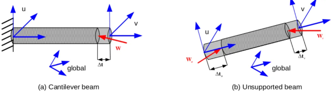
In classical mechanics, the stiffness properties of the cantilever beam (fixed at one side, see Figure 1a) are described by the Hook’s law that defines a linear relation between the applied external wrench (force/torque) W and corresponding deflection t at the free-end

 

W K t (1)

where K is

6 6



x F Fy z F  F and torque [ , , ]T x My Mz M  M components. u v

(a) Cantilever beam (b) Unsupported beam

t W u t v t u W v W u v global global

Fundamentals of manipulator stiffness modeling using matrix structural analysis

In general case, the stiffness matrixKfrom the Hook’s law is symmetric and positive definite but may include a number of off-diagonal elements [37]. For typical beams commonly used in practice (with regular cross-section) the stiffness matrix can be computed analytically as follows

3 2 3 2 2 2 , 0 0 0 0 0 12 6 0 0 0 0 12 6 0 0 0 0 0 0 0 0 0 6 4 0 0 0 0 6 4 0 0 0 0 u v E S L E Iz E Iz L L E Iy E Iy L L G J L E Iy E Iy L L E Iz E Iz L L       _{    }                _               _{    }        K (pourquoi u, v ?) (2)

where L the beam length, S is the beam cross-section area, Iy , Iz are the second moments, J is the polar moment, E and G are Young’s and Coulomb’s modules of the beam material, respectively.

It should be also stressed that for the cantilever beam, both the wrench W and deflection t are usually expressed with respect to the coordinate system attached to the beam’s fixed-end. However, in general case, the vectors W and tmay be presented in the global coordinate system, which requires some revision of (1) and (2). In fact, for small angular displacements, the deflection and wrench vectors in the global system can be presented as

global 3 3 global 3 3 6 6        _        _ _ _ _    p R 0 p φ 0 R φ (3) global 3 3 global 3 3 6 6      _      _ _  _{ }    F R 0 F M 0 R M (4)

where the orthogonal matrix R defines the orientation of the local coordinate system relative to the global one. The letter allows us to present the stiffness model of the cantilever beam in the global coordinate system

global 3 3 3 3 global 6 6 global 3 3 6 6 3 3 6 6 global T T              _  _      _ _ _        F R 0 R 0 p M 0 R K 0 R φ (5)

that gives a simple rule for transforming the local stiffness matrices of all mechanical components to a single coordinate frame. For the unsupported beams (with two non-fixed ends, see Figure 1b) that are used in Matrix Structural Analysis (MSA) as principal components, it is necessary to define the deflections and wrenches for both sides. The latter will be further referred to as “u” and “v” or “1” and “2”. In this case, the stiffness model is presented in an extended form

1 11 12 1 2 21 22 12 12 2    _  _       _       W K K t W K K t (6)

that relates the deflections on both sides t₁,t₂ and corresponding wrenches W W₁, ₂ by means of 12 12 extended stiffness matrix composed of four

6 6



1, 2

W W should satisfy the static equilibrium equation that defines linear dependence between the matrix rows in eq. (6).

To find the desired

6 6



6 6



1 12 2 2 22 2       W K t W K t (7)

Relevant static equilibrium equation is written at the point “1” allows us to express the wrenches W W₁, ₂ via the force F₂ and torque

2 M at the point “2” as 2 2 1 2 2 2 2 ;      _{ } _{ }       F F W M L F W M (8)

where L is the beam length vector directed from the point “1” to the point “2” (i.e. along the beam principal axis). Applying further the cantilever beam standard equation W₂Kt₂ one can get explicit expressions for the matrices K₁₂,K₂₂:

Fundamentals of manipulator stiffness modeling using matrix structural analysis 3 3 22 3 3 3 22 12 3 ; [ ]T       _{   }    I 0 K K K K L I (9)

where [L]denotes the 3 3 skew-symmetric matrix derived from the vector L .

Similarly, in the second case, the global system is located at the right-end of the beam (with the same orientation as in the previous case), which yields  t₂ 0 and simplifies eq. (6) to

1 11 1 2 21 1       W K t W K t (10)

The static equilibrium equation leads to the following expressions

2 1 1 1 1 1 1 ;      _{ } _{   }     F F W W M M L F (11)

where L is the same beam length vector (directed from the point “1” to point “2”). However, the cantilever beam equation should be slightly modified to take into account standard directions of the coordinate axes

3 3 3 3 3 1 3 1 3 3 z z z z                        R 0 R 0 W K t 0 R 0 R (12)

where R_z diag( 1, 1, 1)  is 3 3 rotation matrix around z axis by the angle , which changes directions of the axes x, y. The latter allows us to obtain explicit expressions forK₁₁, K₂₁

 

The physical interpretation of the matrices K₁₁,K₁₂,K₂₁,K₂₂ can be done in the following way. The stiffness matrix K₁₁ describes the force/torque reaction at the beam left-end point caused by the left-end deflection t₁. The stiffness matrix K₁₂describes the force/torque reaction at the beam left-end point caused by the right-end deflection t₂. The stiffness matrix K₂₁describes the force/torque reaction at the beam right-end point caused by the left-end deflection t₁. The stiffness matrix K₂₂describes the force/torque reaction at the beam right-end point caused by the right-end deflection t₂ . The physical meaning of

11, 12, 21, 22

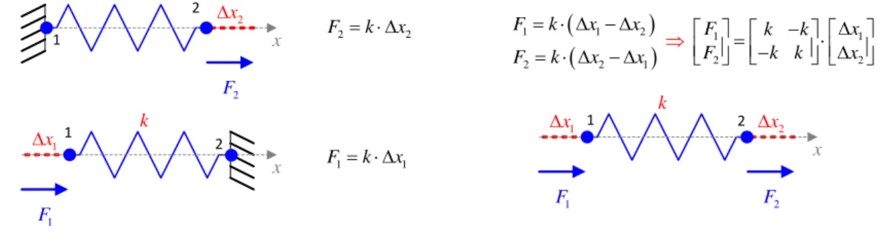
K K K K is also illustrated for the simplest case of the 1D linear spring (Figure 2), where

6 6



x x x 2 x  1 x  x1 x2 2 F 1 F F1 F2 2 2 F   k x k k k 1 1 F   k x









Figure 2 Stiffness models of a simple spring with fixed and free ends

For the beam with a regular shape (with uniform cross-section) the above stiffness matrices can be computed analytically using the following expressions

Fundamentals of manipulator stiffness modeling using matrix structural analysis 3 2 3 2 11 2 2 0 0 0 0 0 12 6 0 0 0 0 12 6 0 0 0 0 0 0 0 0 0 6 4 0 0 0 0 6 4 0 0 0 0 E S L E Iz E I L L E Iy E Iy L L G J L E Iy E Iy L L E Iz E Iz L L       _{   }                 _                _{   }        K (14) 3 2 3 2 12 2 2 0 0 0 0 0 12 6 0 0 0 0 12 6 0 0 0 0 0 0 0 0 0 6 2 0 0 0 0 6 2 0 0 0 0 E S L E Iz E Iz L L E Iy E Iy L L G J L E Iy E Iy L L E Iz E Iz L L        _{    }                  _{ }               _{    }        K (15) 3 2 3 2 21 2 2 0 0 0 0 0 12 6 0 0 0 0 12 6 0 0 0 0 0 0 0 0 0 6 2 0 0 0 0 6 2 0 0 0 0 E S L E Iz E Iz L L E Iy E Iy L L G J L E Iy E Iy L L E Iz E Iz L L        _{     }                 _{ }                _{   }        K (16) 3 2 3 2 22 2 2 0 0 0 0 0 12 6 0 0 0 0 12 6 0 0 0 0 0 0 0 0 0 6 4 0 0 0 0 6 4 0 0 0 0 E S L E Iz E I L L E Iy E Iy L L G J L E Iy E Iy L L E Iz E Iz L L       _{    }                _               _{    }        K (17)

where all notations have the same meaning as in the cantilever beam stiffness matrix (2).

Similar to the cantilever bean case, the stiffness matrix of the unsupported beam can be transformed to the global system using an extended version of eq. (5)

Fundamentals of manipulator stiffness modeling using matrix structural analysis

global global local local

11 12 11 12

global global local local

21 22 21 22 T T T T            _{  }       _{  }           _{ }   R 0 0 0 R 0 0 0 K K 0 R 0 0 K K 0 R 0 0 0 0 R 0 K K K K 0 0 R 0 0 0 0 R _{0 0 0 R} (18)

where the orthogonal matrix R defines the orientation of the local coordinate system relative to the global one.

2.2

MSA-based stiffness models of simple linkages

2.2.1

Two-link serial system with rigid connection

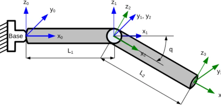
Now let us apply the MSA method to a mechanical system composed of two beam elements of lengths L1, L2 with the rigid connection between them (Figure 3). It is assumed that the beams are not aligned and the angle between them is equal to q. Here, each beam has two local coordinate systems: 0, 1 for the first beam and 2, 3 for the second one, as shown in Figure 3.

Base x0 y0 z0 y1, y2 z1 z3 x3 y3 z2 x1 q L1 x2

(il n’y a pas de points sur la figure) Figure 3 Two-link serial system with rigid connection

Let us assume that the global coordinate system is located at the left-end of the first beam (point 0) and the global coordinate axes are aligned with the local ones. Under this assumption, the force deflection relations for the first link can be written as

1 1 0 11 12 0 1 1 1 21 22 1     _{ }      _        W K K t W K K t (19)

where the upper superscript denotes the link number and relevant matrices are computed using eqs. (14)-(17). For the second beam, the similar relation should be written taking into account that the local axes ( ,x z_{2 2}) and ( ,x z_{3 3}) are turned with respect to the global ones. This yields the following force-deflection relation

2 2 2 11 12 2 2 2 3 21 22 3 T T T T            _{ }      _         W Q K Q Q K Q t W Q K Q Q K Q t (avec K 1

la matrice de rigidité de la poutre 1 et K2 la matrice de rigidité de la

poutre 2) (20)

where ( q, q)

y y

diag 

Q R R is the 6 6 matrix that is expressed via the orthogonal rotation matrix q y

R describing rotation around y-axis by the angle q . For further convenience let us denote K2_ijq Q K _i2_jQ and rewrite the above equation in a more compact T form 2 2 2 11 12 2 2 2 3 21 22 3 q q q q     _{ }      _        W K K t W K K t (21)

After collecting equations (19) and (21) in a single system one can get

1 1 11 12 6 6 6 6 0 0 1 1 21 22 6 6 6 6 1 1 2 2 2 6 6 6 6 11 12 2 2 2 3 24 1 6 6 6 6 21 22 24 24 3 24 1 q q q q                       _        _                 _{ }   K K 0 0 W t K K 0 0 W t W 0 0 K K t W _{0 0 K K} t

(doit on écrire la deuxième dimension pour un vecteur?) (22)

Further, taking into account the boundary condition  t₀ 0 the above system can be reduced down to

1 22 6 6 6 6 1 1 2 2 2 6 6 11 12 2 2 2 3 18 1 6 6 21 22 _{18 18} 3 18 1 q q q q      _             _{  }      _      _{ }   K 0 0 W t W 0 K K t W 0 K K t (23)

Fundamentals of manipulator stiffness modeling using matrix structural analysis

Furthermore, the rigid connection between the beams yields relations   t₁ t₂ and W₁ W₂, where the last one directly follows from Newton's third law. The latter agrees on us to sum-up the first and second lines in the system (23) and obtain the final expression allowing us to compute deflections at the beam ends caused by external loading W₃ applied to the free end of the considered 2-beam system 1 2 2 2 22 11 12 2 2 3 121 21 22 1212 3 121 q q q q           _{ }       _       t K K K 0 W K K t (24)

It is worth mentioning that here the 12 12 matrix is invertible, and equations can be easily solved with respect to the deflections

2, 3

t t . In particular, an analytical solution for the free-end deflection t₃ caused by W₃ may be presented in the following form

3 C 3

W K t (25)

where K_C is the Cartesian stiffness matrix of the two-link system under study





that depends on both beams stiffness parameters included in the matrices K1_ij,K_ij2qand relative orientations of the links described by the matrix Q. It is worth mentioning that here the matrix K_C is non-singular and invertible.

Hence, for this simplest case study, the MSA approach allowed rather easy compute the system stiffness matrix. It is clear that this approach can be also generalized for the multi-beam serial systems with rigid connections, however, the final analytical expression will include the matrix inversion of higher dimension. Besides, it is worth mentioning that the above-presented example implements the general MSA assembling technique that usually produces the matrices similar to (24), which includes a number of matrix sums.

2.2.2

Two-link serial system with a passive joint

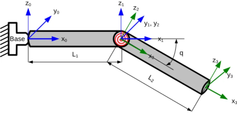
Let us apply the MSA method to a mechanical system composed of two beam elements of lengths L1, L2 with a revolute passive joint between them (Figure 4). In structural mechanics, this type of connection is also called as a pin joint. It is assumed that the passive joint axis is directed along y1 and y2, the beams are not aligned and the angle between them is equal to the passive joint coordinate q . It is worth mentioning that this problem cannot be solved straightforwardly using the standard MSA method, which was primary designed for rigid and elastic connections. However, it is possible to apply some special techniques to adjust MSA for the passive joint case. Base x0 y0 z0 y1, y2 z1 z3 x3 y3 z2 x1 q L1 _x 2

Figure 4 Two-link serial system with a passive joint It is clear that the basic MSA equations for this 2-beam system have the same structure as above

1 22 6 6 6 6 1 1 2 2 2 6 6 11 12 2 2 2 3 18 1 6 6 21 22 _{18 18} 3 18 1 q q q q      _    _         _{  }      _      _{ }   K 0 0 W t W 0 K K t W 0 K K t (27)

but here the matrices K_ij2q are not constant and depend on the passive joint coordinate q, which may vary under the influence of the external loading W₃. However, in contrast to the previous case, where the connection is described by equations   t₁ t₂ and

1  2

W W, here these relations must be replaced by









where the matrices Λr diag(1,1,1,1, 0,1) and Λp diag(0, 0, 0, 0,1, 0) describe the passive joint geometry, and the superscripts ‘r’ and ‘p’ are referred to the “rigid” and “passive” connections. The first of these relations takes into account that the connection 1 and 2 ensures equality of all components of t₁,t₂ except of  1_y, 2_y (since the passive joint axis is directed along y axis). The second

Fundamentals of manipulator stiffness modeling using matrix structural analysis

group of relations shows that the passive joint ensures the validity of the 3rd Newton law for five wrench components only (except of

y

M ), but the torques 1 y

M and 2 y

M are equal to zero. It should be noted that in general case the matrices _Λr _{and Λ}p _{may be}

non-diagonal, but their rank remains the same and is equal to 5 and 1, respectively (as in the case of diagonal matrices). Combining equations (27) and (28) one can get the following linear system

6 6 1 22 6 6 6 6 1 2 2 2 6 6 11 12 1 2 2 3 18 1 22 11 12 2 2 3 30 1 _{6 6 21 22} 1 30 8 q q q q r r p p p q r q r r              _{ }   _{ }     _{      }   _{   }       _{ }       _{ }  Λ Λ 0 0 Λ K 0 0 t 0 0 0 Λ K Λ K t 0 _{Λ K Λ K Λ K} t W _{0 K K} (29)

that should be solved with respect to t₃. It should be mentioned that here the system matrix is non-square (of the size 30 18 ), but it contains 12 zero rows that are caused by zero diagonal components in _Λr _{and Λ}p _{(each Λ}r _{produces one zero-row and each Λ}p

produces five zero-rows). To eliminate the zero-rows that are useless here, let us introduce the modified non-singular matrices





and rewrite the system (29) in the reduced form (with a square matrix of size 18 18 )

* * 5 6 5 1 1 * 22 1 6 1 6 1 1 1 2 2 1 1 1 6 * 11 * 12 2 1 2 2 5 1 * 22 * 11 * 12 3 18 1 2 2 3 _{18 1} 6 6 21 22 ₁₈₁₈ q q r r p p p r q r q q q r        _   _           _{   }   _{     }     _{ }      _    _{  }     _ _  Λ Λ 0 0 Λ K 0 0 0 t 0 0 Λ K Λ K t 0 Λ K Λ K Λ K t W _{0 K K} (31)

This system can be presented in more compact form after defining relevant block matrices

1 12 1 2 3 18 1 18 8 3 18 1 1          _  _{  }   _ _{  }   _{ } t 0 A B t W C D t (32) where * * 5 6 1 1 6 * 22 1 6 2 2 * 12 1 6 * 11 2 1 2 * 12 12 * 22 * 11 12 2 2 6 6 6 12 21 _{6 12} 22 ; ; r r p p p r r r q q q q q q                       _                  _    Λ Λ 0 0 Λ K 0 A B Λ K 0 Λ K Λ K Λ K Λ K C 0 K D K (33)

Further, after elimination t₁,t₂ one can get the following expression for the wrench applied to the system end-point

3 C 3 W K t (34) where 1 C      K D C A B (35)

is the desired Cartesian stiffness matrix of the two-link system under study. It has a similar structure as (26) corresponding to the case of the rigid connection. However, it is easy to verify numerically that here the stiffness matrix K_C is rank-deficient, which is the result of the passive joint connection.

Hence, for this case study, some modification of the MSA approach allowed us to compute the rank deficient stiffness matrix. However, relevant transformations include a number of non-trivial steps, which will be generalized in the following Sections.

Fundamentals of manipulator stiffness modeling using matrix structural analysis

2.2.3

Two-link serial system with an elastic joint

Let us apply the MSA method to a mechanical system composed of two beam elements of lengths L1, L2 with an elastic joint between them (Figure 5). It is assumed that the elastic joint axis is directed along y1 and y2, the beams are not aligned and the angle between them is equal to the elastic joint coordinate q.

It is clear that the basic MSA equations for this 2-beam system have the same structure as in the cases (a) and (b)

1 22 6 6 6 6 1 1 2 2 2 6 6 11 12 2 2 2 3 18 1 6 6 21 22 _{18 18} 3 18 1 q q q q      _    _         _{  }      _      _{ }   K 0 0 W t W 0 K K t W 0 K K t (36)

Here the matrices K2q_ij are not constant and depend on the elastic joint coordinate q, which may vary under the influence of the external loading W₃. However, in contrast to the cases of the rigid and passive connections, here the joint static equations must be replaced by





where K is the stiffness coefficient of the elastic joint, the matrices _{q Λ}r _diag(1,1,1,1, 0,1) _{and Λ}e _{diag(0, 0, 0, 0,1, 0) describe}

the passive joint geometry, and the superscripts ‘r’ and ‘e’ are referred to “rigid” and “elastic” connections. The first of these relations takes into account that the connection 1 and 2 ensures equality of all components of t₁,t₂ except of 1_, 2

y y

  (since the elastic joint axis is directed along y). The second group of relations shows the elastic joint ensures validity of the 3rd Newton law for all wrench components, and the third relation describes the Hooke’s law for the elastic joint.

Base x0 y0 z0 y1, y2 z1 z3 x3 y3 z2 x1 q L1 x2

Figure 5 Two-link serial system with an elastic joint After combining equations (36) and (37) one can get the following linear system

6 6 2 2 1 11 12 2 1 2 2 22 11 12 3 18 1 2 2 3 24 1 _{6 6 21 22} 8 24 1 q q q q q q r r e e e e q q K K     _      _{   }   _    _{  }      _{   }   _{  } _  _    _ Λ Λ 0 0 t Λ Λ K Λ Λ K 0 t 0 _{K K K} t W _{0 K K} (38)

that should be solved with respect to t₃. It should be mentioned that here the system matrix is non-square of the size 24 18 , but it contains 6 zero rows that are caused by zero diagonal components in _Λr _{and Λ}e _{(each Λ}r _{produces one zero-row and each Λ}e

produces five zero-rows). To eliminate the zero-rows that are useless here, let us introduce the modified non-singular matrices Λ of _*r the size 5 6 (see eq. (30)) and Λ_*e 





* * 6 6 5 1 2 2 ₁ * * 11 * * 12 1 1 2 1 2 2 6 1 _{22 11 12} 3 2 2 18 1 3 _{18 1 6 6 21 22} 8 18 1 q q q q q r r e e e e q q q K K              _{ }     _    _{  }      _{ }     _{ }       _{ }   Λ Λ 0 0 t Λ Λ K Λ Λ K 0 t 0 _{K K K} t W _{0 K K} (39)

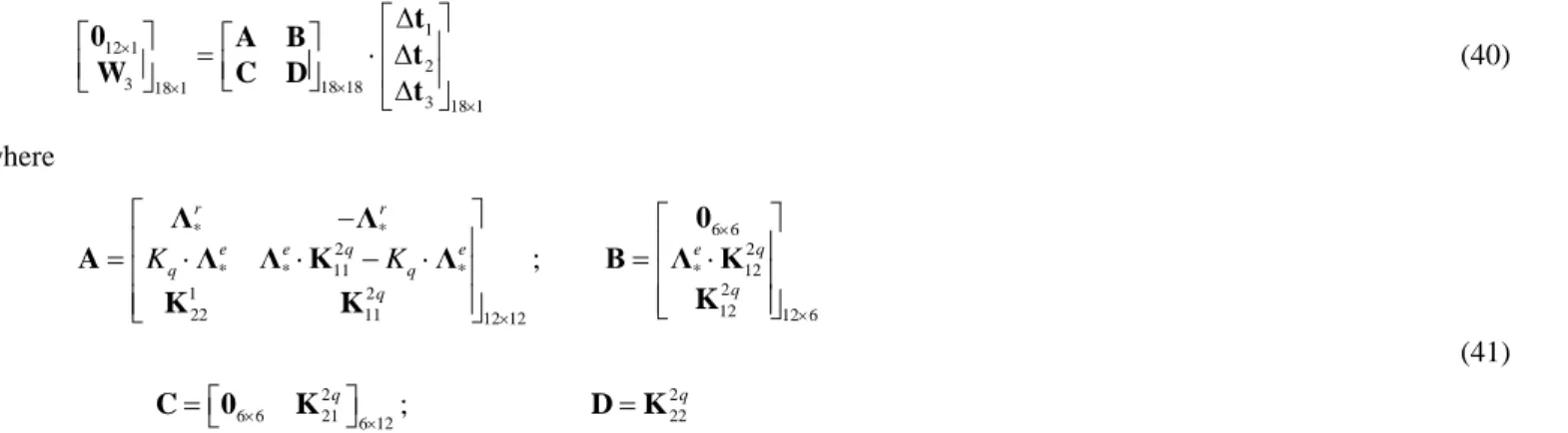
Fundamentals of manipulator stiffness modeling using matrix structural analysis 1 12 1 2 3 18 1 18 8 3 18 1 1          _  _{  }   _ _{  }   _{ } t 0 A B t W C D t (40) where 6 12 6 6 * * 2 2 * * 11 * * 12 2 1 2 12 22 11 12 12 2 2 6 6 21 _{6 12} 22 ; ; r r e e q e e q q q q q q q K K               _   _ _  _               0 Λ Λ A Λ Λ K Λ B Λ K K K K C 0 K D K (41)

Further, after elimination t₁,t₂ one can get the following expression for the wrench applied to the system end-point

3 C 3 W K t (42) where 1 C      K D C A B (43)

is the desired Cartesian stiffness matrix of the two-link system under study. It has a similar structure as (26) and (35) corresponding to the cases of the rigid and passive connections. It is easy to verify numerically that here the stiffness matrix K_C is full-rank, which is in a good agreement with the nature of the elastic joint.

2.2.4

Two-link parallel system with passive joints

Let us apply the MSA method to a closed-loop mechanical system composed of two beam elements with three revolute passive joints, which connect the beams to the rigid base at the left-hand side and to the end-effector on the right-hand side (Figure 6). It is assumed that the passive joint axes are directed along y and the angle between the beams is equal to q.

Base Base x0 y0 z0 y1, y3 z1 z3 x1 q L1 x2 x2 y2 z2

Figure 6 Two-link parallel system with passive joints Similar to all previous cases the basic elasto-static equations and are written as follows

1 1 11 12 6 6 6 6 0 0 1 1 21 22 6 6 6 6 1 1 2 2 2 6 6 6 6 11 12 2 2 2 3 24 1 6 6 6 6 21 22 24 24 3 24 1 q q q q                       _        _                 _{ }   K K 0 0 W t K K 0 0 W t W 0 0 K K t W _{0 0 K K} t (44)

where the matrices K2q_ij depend on the system geometric parameter q. However, because of the non-rigid connections between the beams and the base, here  t₀ 0 and  t₂ 0 that does not allow us to reduce the matrix dimension in a trivial way (as it was done in all previous examples, where the lines corresponding to W₀ were simply removed).

For the considered system, the left-hand side connections between the beam and rigid base (via the passive joints) produce the following equations 0 2 0 2 ; ; r r p p           Λ t 0 Λ t 0 Λ W 0 Λ W 0 (45)

Fundamentals of manipulator stiffness modeling using matrix structural analysis

where the first group describes the passive joint geometry and the second group follows from the 3rd Newton’s law (the matrices _Λr

and _Λp _{are defined above in the example (b)). For the right-hand side connections between the beams and end-effector, it is}

necessary to define additional variables t and W_e describing the end-effector deflection and wrench, respectively. Using these notations, the end-effector wrench may be expressed as follows

r ( _{3 1})

e  

W Λ W W (46)

Besides, the passive joint geometry and the 3rd Newton’s law at the right-hand side yield equations









that allows us to take into account particularities of the end-effector connection. Combining equations (44)-(47) yields the following linear system

6 1 _{6 6 6 6 6 6 6 6} 6 1 6 6 6 6 6 6 6 6 6 1 6 6 6 6 6 6 6 1 6 6 6 6 6 6 1 1 6 1 11 12 6 6 6 6 6 6 6 1 1 1 21 22 6 6 6 6 6 6 6 1 6 6 6 6 11 6 1 6 1 54 1 r r r r r r p p p p p e  _{   }  _{   }  _{  }                              _                  0 _{Λ 0 0 0 0} 0 _{0 0 Λ 0 0} 0 _{0 Λ 0 0 Λ} 0 0 0 0 Λ Λ 0 Λ K Λ K 0 0 0 0 Λ K Λ K 0 0 0 0 0 0 Λ K 0 0 W 0 1 2 3 2 2 30 1 12 6 6 2 2 6 6 6 6 21 22 6 6 1 1 2 2 21 22 21 22 6 6 54 30 q p p p r r r q r q q q q                    _{ }   _{ }     _{ }   _ _   _{ }         t t t t t Λ K 0 0 0 Λ K Λ K 0 Λ K Λ K Λ K Λ K 0 (48)

that should be solved with respect to t. It should be mentioned that here the system matrix is non-square of the size 54 30 , but it contains 24 zero rows that are caused by zero diagonal components in _Λr _{and Λ}p _{(each Λ}r _{produces one zero-row and each Λ}p

produces five zero-rows). To eliminate the zero-rows, let us use the modified non-singular matrices _{Λ and *}r * p

Λ (defined in example (b)) and rewrite the system (48) in the reduced form

* 5 6 5 6 5 6 5 6 5 1 5 6 5 6 * 5 6 5 6 5 1 5 6 * 5 6 5 6 * 5 1 5 6 5 6 5 6 * * 5 1 1 1 1 1 * 11 * 12 1 6 1 6 1 6 1 1 1 1 * 21 * 22 1 6 1 6 1 6 1 1 1 6 1 6 1 1 30 1 r r r r r r p p p p e                        _{  }  _{ }         _                     Λ 0 0 0 0 0 0 0 Λ 0 0 0 0 Λ 0 0 Λ 0 0 0 0 Λ Λ 0 0 Λ K Λ K 0 0 0 0 _{Λ K Λ K 0 0 0} 0 _{0 0 Λ} 0 W 0 1 2 3 2 2 30 1 * 11 * 12 1 6 2 2 1 6 1 6 * 21 * 22 1 6 1 1 2 2 21 22 21 22 6 6 _{30 30} p p p p r r r q q q q r q q       _             _{ }   _{ }     _{ }   _ _   _{ }         t t t t t K Λ K 0 0 0 Λ K Λ K 0 Λ K Λ K Λ K Λ K 0 (49)

where the main matrix of size 30 30 is obviously rank-deficient (since the 29th column is equal to zero). The latter is in a good agreement with physical nature of the system, where the end-effector is connected to the beams via the passive joints. To obtain the final expression, the reduced system can be presented in a compact form

0 1 24 1 2 30 1 3 30 0 8 1 3 1 e        _    _  __    _ _     _{ }     t t 0 A B t W C D t t (50)

Fundamentals of manipulator stiffness modeling using matrix structural analysis * 5 6 5 6 5 6 _{5 6} 5 6 5 6 * 5 6 5 6 5 6 * 5 6 5 6 * 5 6 5 6 5 6 * 1 1 * 11 * 12 1 6 1 6 1 1 * 21 * 22 1 6 1 6 2 2 1 6 1 6 * 11 * 12 2 2 1 6 1 6 * 21 * 22 24 24 ; r r r q r r p p p q q q p p p p p    _                               _                Λ 0 0 0 ₀ 0 0 Λ 0 0 0 Λ 0 0 _Λ 0 0 0 Λ _Λ A B Λ K Λ K 0 0 Λ K Λ K 0 0 0 0 Λ K Λ K 0 0 Λ K Λ K 6 * 1 6 1 6 1 6 1 6 24 1 1 6 2 2 2 21 22 21 22 ₄; 6 6 r r r q r r q                                _{ }  0 0 0 0 C Λ K Λ K Λ K Λ K D 0 (51)

Further, after elimination t₀, t₁, t₂,t₃ one can express the end-effector wrench as

C e  W K t (52) where 1 C      K C A B (53)

is the desired Cartesian stiffness matrix of the two-link closed-loop system under study. It has a similar structure as in the above examples. Also, it is easy to prove analytically that the stiffness matrix K_C is rank-deficient (here rank( )B 5 because of a zero column), which is the result of the passive joint connection to the end-effector.

Summarising all above-presented case studies, one can conclude that some modifications of the MSA approach allowed us to obtain the desired Cartesian stiffness matrix that may be either a full-rank or rank-deficient one. However, relevant techniques include a number of non-trivial steps, which will be generalized in the following Section to be applied to more complex structures.

2.3

General methodology of classical MSA

As follows from the above case studies, basic ideas of the classical MSA can be successfully used in robotics but some enhancement is required in order to take into account numerous passive and actuated connections. Before presenting the proposed enhancement, let us remind briefly basic steps of the classical MSA that is perfectly suited for computer-aided analysis of complex structures such as trusses, bridges, high voltage towers, etc. In general, the MSA based stiffness analysis includes the following steps:

Step 1: Decoupling the original system into generic structural members such as beams, rods, etc. and presenting the system as a set of member elements connected at the nodes (MSA idealization).

Step 2: Creating “free-free” master stiffness models for each element using 12 12 stiffness matrices and presenting them in the global coordinate system (MSA members modeling).

Step 3: Creating the node-element connectivity matrix that defines links between model members via rigid, elastic or passive connections (MSA members connecting).

Step 4: Merging the individual stiffness matrices to the global stiffness matrix for the entire structure using the node-element connectivity matrix and overlapping technique (MSA assembling).

Step 5: Defining nodal loads and system supports, incorporating them in the global stiffness model, application of the boundary conditions/constraints and reducing the global stiffness matrix dimension (MSA constraints).

Step 6: Solving the resulting set of the reduced equations for unknown nodal displacements corresponding to given external loads (MSA solving).

Step 7: Computing reaction forces at the supports, the nodal internal forces and stresses for all system members (MSA post-processing).

It should be noted that practical computer implementation of the MSA method significantly differs from the manual technique presented in the previous Section. There are two main differences: (i) at the assembling stage the individual stiffness matrices are not expanded but are directly merged through the use of special “freedom pointer array”; (ii) both the individual and global stiffness matrices are stored using a special format that takes advantage of symmetry and sparseness. There are also some differences in the application of boundary conditions and the global stiffness matrix reduction. Nevertheless, relevant computer-oriented routines ensure satisfaction of two basic rules of structural mechanics: compatibility of displacement and force equilibrium, which are equivalent to the simple merging of 6-dimensional rows and columns in the global stiffness matrix. Hence, some modifications of these routines are required to apply MSA in robotics where the size of the global stiffness matrix is not very high but the connections between the structural members (passive and actuated joints) should be treated in a different manner.

Fundamentals of manipulator stiffness modeling using matrix structural analysis

3

MSA enhancement for robotic manipulators

In contrast to structural mechanics where the main interest is in the area of the nodal displacements, reaction/internal forces and stresses, the stiffness analysis in robotics concentrates on computing of the Cartesian stiffness matrix defining the force-deflection relation for the manipulator end-effector. Let us present the MSA based technique adapted for robotic applications, which is issues from previous works [18, 38] and also contains some new contributions and generalizations.

3.1

MSA models of manipulator links and platforms

3.1.1

Modeling of a flexible link

If the link flexibility is non-negligible, the 2-node “free-free” stiffness model should be used, which can be obtained either from the approximation of the link by a beam or using the CAD-based technique [9] allowing to evaluate the stiffness parameters taking into account the link real shape and geometry. In both cases the link is described by the linear matrix equation, containing 12 12

“free-free” stiffness matrix

( ) ( ) 11 12 ( ) ( ) 21 22 1212 ij ij i i ij ij j _ j     _{ }      _        W K K t W _{K K} t (54)

where t_i,t are the deflections at the link ends, _j W W are the link end wrenches, i and j are the node indices corresponding to _i, _j the link ends, and ( ) ( ) ( ) ( )

11 , 12 , 21, 22 ij ij ij ij

K K K K are

6 6



It is clear that in general case when the link is arbitrary oriented with respect to the global coordinate system, the above equations should be slightly modified by simply rotating the local stiffness matrices

( ) ( ) ( ) ( ) ( ) ( ) ( ) ( ) 11 12 11 12 ( ) ( ) ( ) ( ) ( ) ( ) ( ) ( ) 21 22 21 22 g ij g ij ij ij ij ij ij ij g ij g ij ij ij ij ij T T i ij T T j                      K K Q K Q Q K Q K K Q K Q Q K Q (55) where ( )ij ( ( )ij, ( )ij) diag 

Q R R is composed of two similar orthogonal matrices ( )ij

R defining the orientation of the local coordinate system of the link (ij) relative to the global one and left superscript “g” indicates that matrix is presented in the global coordinate system.

3.1.2

Modeling of a rigid link

If the link flexibility is negligible, the above stiffness model should be replaced by two types of equations describing the displacement and force equilibriums. The first of them can be treated as a simple “rigidity constraint” that keeps constant the distance between the nodes i and j. Applying to this link the rigid body kinematic equations, one can get the following relations between the nodal displacements ti [pi;φi], tj [pj;φj] expressed via the linear and angular components

( ) j i ij j i i         φ φ p p φ d (56)

where the vector d( )ij [d_x( )ij,d( )_yij,d_z( )ij]T describes the link geometry and is directed from the ith to jth node. This constraint can be also rewritten in the matrix form

3 3 3 3 3 3 6 1 3 3 3 3 3 3 3 3 ( ) _] [ i T j j i              _ _  _  _ _   I d t I 0 I t I 0 0 0 (57)

where _[d( )ij_{] denotes the}

3 3 skew-symmetric matrix derived from the vector ( )ij

d . Further, after definition 6 6 block matrix

( ) _{3 3} 3 3 3 ) 3 6 ( 6 [ j ]T ij _ i        _I d _ D 0 I (58)

the displacement constraint for the rigid-link can be presented in the following form

( ) 6 6 6 1 ij i j        _{ } D I  _tt _ 0 (59)

that is convenient for further aggregation of the stiffness model components.

The second group of equations describing the force equilibrium can be derived using the rigid body static equations, which yields the following relations

Fundamentals of manipulator stiffness modeling using matrix structural analysis ( ) ₀ 0 ij j i j j i       F F d M M F (60)

where F F_i, _j and M M_i, _j denote the forces and torques applied at the nodes i and j respectively. In a matrix form, they can be presented as follows ( ) 0 0 ij i   j   _{ }     I W W I d (61)

Similarly, using the above-introduced definition for ( )ij

D , this equation can be rewritten in a more compact form

( )

6 1 ij T

iD j 0

W W (62)

Hence, the rigid link produces 12 scalar equations describing the displacement and force equilibriums

( ) 6 6 6 1 ( ) 6 6 6 1 ij i j ij T i j          _{ }   _ _     _{ }  _{  } D I D t W W I 0 t 0 (63)

which are written with respect to 24 scalar variables contained in six-dimensional vectors t_i,t_j and W W_i, _j , similar to the flexible link case (the rank deficiency of the matrix is also equal to 12 here).

3.1.3

Modeling of a rigid mobile platform

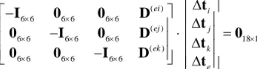
If the platform can be treated as a rigid body, it can be included in the global stiffness model by means of several virtual rigid links connecting the nodes i j k, , ,... of the manipulator leg clamping points and the virtual rigid node e corresponding to the manipulator end-effector reference point (see Figure 7a). From the displacement equilibrium, one can derive several equations similar to (59) that may be aggregated in a common matrix equation

( ) 6 6 6 6 6 6 ( ) 6 6 6 6 6 6 18 1 ( ) 6 6 6 6 6 6 ei i ej j ek k e                _{ }   _ _{ }   _{ }      _ _ I 0 0 D 0 I 0 D 0 0 0 I D t t t t (64)

where _D( )ei_,D( )ej _,D(ek) _{describe the virtual links geometry in the same way as in (58). However, the force equilibrium produces here}

a single equation only

( ) ( ) ( ) 6 1 ei T ej T ek T j e i D kW   D W D W W 0 (65)

which is an extended form of (62). In a matrix form, it can be presented as

( ) ( ) ( ) 6 6 6 1 i ei T ej T ek T j k e                   W W D D D I 0 W W (66)

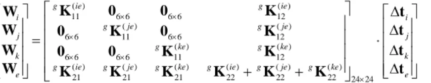
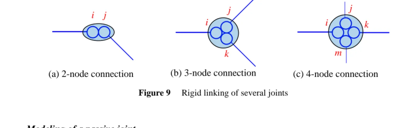
Hence, for this example where the number of the leg clamping points is assumed to be equal to three, the model includes 24 scalar equations and 48 scalar variables. The rank deficiency of the model matrix is equal to 24, which agrees with the rigid body mechanics. It is clear that this model can be easily generalized to the case of 4, 5, … of attached legs by straightforward expanding the matrix sizes. e i k j e3 e1 e2 d(ie) d(ke) d(je) e i k j e3 e1 e2 K(ke) K(je) K(ie)

(a) rigid platform (b) non-rigid platform

Chain #1 Chain #2 Chain #3 Chain #1 Chain #2 Chain #3