HAL Id: hal-01390487
https://hal.inria.fr/hal-01390487
Submitted on 7 Nov 2016
HAL is a multi-disciplinary open access
archive for the deposit and dissemination of
sci-entific research documents, whether they are
pub-lished or not. The documents may come from
teaching and research institutions in France or
abroad, or from public or private research centers.
L’archive ouverte pluridisciplinaire HAL, est
destinée au dépôt et à la diffusion de documents
scientifiques de niveau recherche, publiés ou non,
émanant des établissements d’enseignement et de
recherche français ou étrangers, des laboratoires
publics ou privés.
An Application of SMC to continuous validation of
heterogeneous systems
Alexandre Arnold, Massimo Baleani, Alberto Ferrari, Marco Marazza, Valerio
Senni, Axel Legay, Jean Quilbeuf, Christoph Etzien
To cite this version:
Alexandre Arnold, Massimo Baleani, Alberto Ferrari, Marco Marazza, Valerio Senni, et al.. An
Application of SMC to continuous validation of heterogeneous systems. Simutools 2016 - Ninth EAI
International Conference on Simulation Tools and Techniques, Aug 2016, Prague, Czech Republic.
�hal-01390487�
An Application of SMC to continuous validation of
heterogeneous systems
∗Alexandre Arnold
1, Massimo Baleani
2, Alberto Ferrari
2, Marco Marazza
2, Valerio Senni
2, Axel
Legay
3, Jean Quilbeuf
3, Christoph Etzien
41AIRBUS, 2ALES - UTSCE,
3Inria 4OFFIS
ABSTRACT
This paper considers the rigorous design of Systems of Sys-tems (SoS), i.e. sysSys-tems composed of a series of heteroge-neous components whose number evolves with time. Such components coalize to accomplish functions that they could not achieve alone. Examples of SoS includes (among many others) almost any application of the Internet of things such as smart cities or airport management system.
Dynamical evolution of SoS makes it impossible to design an appropriate solution beforehand. Consequently, existing approaches build on an iterative process that takes its evo-lution into account. A key challenge in this process is the ability to reason and analyze a given view of the SoS, i.e. ver-ifying a series of goals on a fixed number of SoS constituents, and use the results to eventually predict its evolution.
To address this challenge, we propose a methodology and a tool-chain supporting continuous validation of SoS behav-ior against formal requirements, based on a scalable formal verification technique known as Statistical Model Checking (SMC). SMC quantifies how close the current view is from achieving a given mission. We integrate SMC with exist-ing industrial practice, by addressexist-ing both methodological and technological issues. Our contribution is summarized as follows: (1) a methodology for continuous and scalable val-idation of SoS formal requirements; (2) a natural-language based formal specification language able to express complex SoS requirements; (3) adoption of widely used industry stan-dards for simulation and heterogeneous systems integration (FMI and UPDM); (4) development of a robust SMC tool-chain integrated with system design tools used in practice. We illustrate the application of our SMC tool-chain and the obtained results on a case study.
∗Research supported by the European Community’s
Sev-enth Framework Programme [FP7] under grant agreement no 287716 (DANSE).
ACM ISBN 978-1-4503-2138-9. DOI:10.1145/1235
Keywords
Systems of systems, statistical model checking, FMI, tool-chain, simulation.
1.
INTRODUCTION
Context and challenges.
A System of Systems (SoS) is a large-scale, geographically distributed set of independently managed, heterogeneous Constituent Systems (CS). Those entities are collaborating as a whole to accomplish functions/goals that could not be achieved otherwise by any of them, if considered alone [26]. Those goals can either be global to the system, or local to some of its constituents. Constituent Systems are loosely coupled and pursue their own objectives, while collaborat-ing for achievcollaborat-ing SoS-level objectives. An SoS adapts itself to its environment through (1) an evolution of the functions provided by its Constituent Systems and (2) an evolution of its architecture. A typical example of an SoS is the Air Traffic Management System of an airport, which coordinates incoming and outgoing aircraft as well as ground-based vehi-cles and controllers. Such an SoS may evolve in order to ac-commodate a larger number of passengers, difficult climatic conditions or a modification in the laws regarding security.
Misbehaviors of the functions provided by an SoS can be dangerous and costly. Therefore, it is important to identify a set of analysis and tools to verify that the SoS implementa-tion meets funcimplementa-tional and non funcimplementa-tional requirements and correctly adapts to changes of the environment during any phase of the design and operation life-cycle. The manager of a SoS should be able to run these analysis in order to take decisions regarding the evolution of the SoS. The main characteristics of an SoS have been long debated since [26]. Nevertheless, one of the key characteristics of an SoS is dy-namical evolution, that is, the fact that Constituent Systems may evolve, leave, fail, or be replaced.
In fact, dynamical evolution of SoS makes it impossible to design an appropriate solution beforehand. Consequently, the design flow of a SoS is reiterated multiple times during the operation of the SoS, in order to adapt to its evolu-tions. As a summary, SoS rigorous design methodologies thus introduce two major challenges. The first one is to check whether a given view of the system (i.e. a fixed num-ber of components) is able to achieve a mission. The second challenge is to exploit the solution to the first challenge in an engineering methodology that permits dynamical evolution
of the system in case new missions are proposed, in case the environment has changed, or in case the current view cannot achieve the mission. This design approach has been followed by the DANSE project which developed a new SoS design and operation methodology [15].
Contributions.
This paper focuses on Challenge one described above, that is to reason on a given view of the system. A corner stone to solve the challenge is to develop a usable language for ex-pressing formal requirements independent from the number and identity of CSs and thus from the architectural choices. In this paper, we propose Goal Contract Requirement Language (GCSL). This is a very expressive pattern-based language to specify requirements on an SoS and its CSs. The language uses an extension of OCL to express con-straints independent of the view such as : “the total fire area (over a set of districts) is smaller than 1 percent of the total area of the districts.”. By combining those constraints with temporal patterns, we express timing requirements on the behaviors of the view. For instance, the GCSL formula “always [SoS.itsDistricts.fireArea→sum()<0.01∗SoS.itsDistricts.area →sum()]” checks that the above constraint is verified at any point of the simulation. A first version of GCSL was intro-duced in [27]. In this paper we propose additional patterns for expressing properties about the amount of time during which a given predicate remains satisfied. We show that GCSL is powerful enough to capture most of SoS goals and emergent behaviors proposed by our industry partners. The reader shall observe that the language can methodologically be extended to capture more requirements on demand.
The second main difficulty is to detect emergent behav-iors and verify the absence of undesired ones. This requires a suitable verification technique. A first solution would be to use formal techniques such as model checking. Unfortu-nately, both the complexity and the heterogeneous nature of the constituent systems prevent this solution. To solve this problem, we rely on Statistical Model Checking (SMC) [37]. SMC works by monitoring executions of the system, and then use an algorithm from the statistics in order to as-sess the overall correctness. Contrarily to classical Valida-tion techniques, SMC quantifies how close the view is from achieving a given mission. This information shall latter be exploited in the reconfiguration process.
The objective of the paper is not to improve existing statistical algorithm, but rather to expand the SMC ver-ifier Plasma [9] which proposes several algorithms such as Monte Carlo or hypothesis testing. In order to implement an SMC algorithm for SoS, one has to propose a simu-lation approach for heterogeneous components as well as a monitoring approach for GCSL requirements. While a GCSL monitor is easily obtained by translating GCSL to Bounded Temporal Logic (BLTL) as in [6], simulating SoS requires that one defines a formal representation for SoS constituents. In this work, we exploit the Functional Mock-up Interface (FMI) [33] standard as a unified representation for heterogeneous systems. In recent years, the develop-ment of DESYRE, a new simulator, provided us joint simu-lation for FMI/FMU. One of the main contributions of the paper is a full integrated tool-chain between the statistical model checker Plasma [9], FMI/FMU, and DESYRE. This tool-chain is, to the best of our knowledge, the first one that offers a full SMC-based approach for the verification of
complex heterogeneous systems.
The third main difficulty of our work is to make sure that the technology will be accepted by practitioners, both in terms of usability and in terms of seamless integration with existing industrial practice and tools. Our first con-tribution provides a solution for expressing requierements. However, we need a language to specify the system itself. In this paper, we propose to support wide-spread industry standards for SoS. This is done by exploiting UPDM [34] for SoS architecture design and the FMI standard for con-stituent systems. We build on Rhapsody which is a tool used to describe UPDM views, that we enrich with prob-ability distribtutions. The latter capture uncertainty on the environment so that the verification accounts for pre-dictions on environment’s evolution. We then integrate the Constituent Systems behavioral models with the UPDM ar-chitecture through the FMI standard. By exploiting our SMC tool chain, we thus provide the full integration of our SMC-based tool for FMI/FMU within Rhapsody.
Our approach has been illustrated on a firefighting SoS, at the scale of a city. The constituent systems are the dis-tricts of the city, the cars, the firemen, the fire stations and the central command center. We show how our tools are used to model the architecture and the constituents systems of the SoS. The architecture indicates how the Constituent Systems cooperate to provide an emergent behavior, namely the extinction of the fires. Using our tool chain, we evaluate the probability of this emergent behavior.
Structure of the paper.
The paper is organized as follows. In Section 2 we pro-vide a summary of the Statistical Model Checking approach adopted in our tool-chain. Following this, in Section 3 we introduce the GCSL formal language for specifying formal requirements on SoS and CSs behavior. Finally, we discuss in Section 4 the SMC tool-chain and its integration with ex-isting industrial tools for System design. This tool-chain is demonstrated on an industrial case study in Section 5, where we show its application to a Fire Emergency Response sys-tem designed in DANSE [2], modeling a complex SoS that manages fire emergencies in a large city.
2.
BACKGROUND ON STATISTICAL MODEL
CHECKING
Analyzing Systems of Systems requires a careful choice of the verification technique to use. A first solution would be to use model checking. However, this formal approach often requires an input written in a dedicated language, which con-flicts with industry acceptance. Even if a complete model were made in a suitable language, analysis would not be feasible because of the very large size of SoSs and its het-erogeneous nature. Therefore, we rely on Statistical Model Checking (SMC), which is a trade off between testing and model checking. SMC works by simulating the system and verifying properties on the simulations. An algorithm from the statistic area exploits those results to estimate the prob-ability for the system to satisfy a given requirement.
The quantitative results provided by SMC is richer than a Boolean one. Indeed, if the system does not satisfy the requirement, a Boolean tool returns “not satisfied” without any evaluation of the probability of a correct behavior.
be-havior of the system is governed by a stochastic semantic, that is the choice of the next state in an execution depends on a probability distribution. This hypothesis shall not be seen as a drawback. Indeed, most of SoS do make stochas-tic assumptions on their external environment or on their hardware. In case no distribution is known, one relies on the uniform distribution which has the maximal entropy.
In the rest of this section, we first present the BLTL logic used to express properties on system’s executions. Then, we present some statistical algorithms used by the SMC engine.
2.1
BLTL Linear Temporal Logic
In this paper, we focus on requirements of SoS that can be verified on bounded executions. This assumption is used to guarantee that the SMC algorithm will terminate. The bounded hypothesis shall not be viewed as a problem. In-deed, like it is the case in the testing world, it is sufficient to consider that the system has a finite live time.
Definition 1. Given a set of variables V and their do-main D, a state σ is a valuation of the variables, that is σ∈ DV. A trace τ is a sequence of states and timestamps
(σ0, t0), · · · , (σk, tk), where ∀i ti∈ R+∧ ti< ti+1.
We present here BLTL, a variant of LTL [30] where each temporal operator is bounded. Properties of SoS will be ex-pressed in GCSL, that instantiates to BLTL (see Section 3). The core of BLTL is defined by the following grammar, where the time subscript t is interpreted as an offset from the time instant where the sub-formula is evaluated: ϕ ::= true | false | p ∈ AP | ϕ1∧ϕ2| ¬ϕ | ϕ1U≤tϕ2| X≤tϕ
Here, AP is a set of atomic predicates defined in Section 3.2. In our case, an atomic predicate depends on the past states. The temporal modalities F (the “eventually”) and G (the “al-ways”) can be derived from the “until” U as Ftϕ= true U≤tϕ
and Gtϕ= ¬Ft¬ϕ, respectively. The semantics of BLTL is
defined with respect to finite traces τ . We denote by τ, i |= ϕ the fact that a trace τ = (σ0, t0), · · · , (σℓ, tℓ) satisfies the
BLTL formula ϕ at point i of execution. The meaning of τ, i|= ϕ is defined recursively:
τ, i |= true and τ, i 6|= false;
τ, i |= p if and only if p(τ, i) (cf. Subsection 3.2); τ, i |= ϕ1∧ ϕ2 if and only if τ, i |= ϕ1 and τ, i |= ϕ2;
τ, i |= ¬ ϕ if and only if τ, i 6|= ϕ;
τ, i |= ϕ1Utϕ2 if and only if there exists an integer j ≥ i such
that (i) tj ≤ ti+ t, (ii) τ, j |= ϕ2, and (iii) τ, k |= ϕ1, for each
i ≤ k < j;
τ, i |= X≤tϕ if and only if τk, 0 |= ϕ where k = min{j > i | tj>
ti+ t} and τk = ((s′0, t′0), · · · , (s′ℓ−k, t′ℓ−k)) with s′i = si+k and
t′ i= ti+k;
Typically, a monitor, such as in [17], is used to decide whether a given trace satisfies a given property.
2.2
Statistical Model Checking
Given a stochastic system M and a property ϕ, SMC is a simulation-based analysis technique [37, 32] that answers two questions: (1) Qualitative : whether the probability p for M to satisfy ϕ is greater or equal to a certain threshold ϑ or not; (2) Quantitative : what is the probability p for M to satisfy ϕ. In both cases, producing a trace τ and check-ing whether it satisfies ϕ is modeled as a Bernoulli random variable Bi of parameter p. Such a variable is 0 (τ 6|= ϕ) or
1 (τ |= ϕ), with P r[Bi = 1] = p and P r[Bi= 0] = 1 − p.
We want to evaluate p.
Qualitative Approach.
The main approaches [36, 32] proposed to answer the qual-itative question are based on Hypothesis Testing. In order to determine whether p ≥ ϑ, we follow a test-based ap-proach, which does not guarantee a correct result but con-trols the probability of an error. We consider two hypoth-esis: H : p ≥ ϑ and K : p < ϑ. The test is parameterized by two bounds, α and β. The probability of accepting K (resp. H) when H (resp. K) holds is bounded by α (resp. β). Such algorithms sequentially execute simulations until either H or K can be returned with a confidence α or β, which is dynamically detected. Other sequential hypothe-sis testing approaches exists, which are based on Bayesian approach [22].
Quantitative Approach.
In [18, 23] Peyronnet et al. propose an estimation pro-cedure to compute the probability p for M to satisfy ϕ. Given a precision ǫ, Peyronnet’s procedure, which we call PESTIM , computes an estimate p′of p with confidence 1−δ,
for which we have: P r(|p′− p|≤ǫ) ≥ 1 − δ. This procedure is
based on the Chernoff-Hoeffding bound [19], which provides the minimum number of simulations required to ensure the desired confidence level.
The quantitative approach is used when there is no known approximation of the probability to evaluate, i.e. to obtain a first approximation. This method is useful when the goal of the analysis is to have a idea on how well the model be-haves. On the contrary, the qualitative approach determines whether the probability is above a given threshold, with a high confidence and in a minimal number of simulations.
3.
TIMED OCL CONSTRAINTS FOR SOS
REQUIREMENTS
The challenge in promoting the use of formal specification languages in an industrial setting is essentially to provide a good balance between expressiveness and usability. In this section we present the requirements language, called GCSL (Goal and Contract Requirement Language). The full GCSL language specification, as well as the details of translation of the GCSL patterns into BLTL, can be retrieved in [3]. In this section we focus on providing a brief recap of the language and illustrate why it is appropriate to define SoS and CSs requirements. We also discuss an explicit contribution of this paper to GCSL.
3.1
A Survey of GCSL
A GCSL contract is a pair of Assume/Guarantee asser-tions denoting requirements on SoS and CSs inputs and outputs, respectively. Contracts allow us to decompose re-quirements and perform local or global verification on need. Assertions are built upon GCSL natural-language patterns, some of which are shown in Figure 1. GCSL patterns are inspired by and extend the Contract Specification Language (CSL) patterns [1], developed in the SPEEDS European project. These natural-language based requirements have their formal semantics defined by translation into correspond-ing BLTL formulas, enablcorrespond-ing the application of SMC. To simplify the specification of properties of complex systems
and architectures, GCSL integrates the Object Constraint Language (OCL) [35], a formal language used to describe static properties of UML models. OCL is an important means to improve the expressiveness and usability of GCSL patterns. Using OCL we can describe properties about types of CS in the SoS architecture, while being independent of their actual number of instances and, thus, defining require-ments that are adaptable to the natural evolution of the SoS, without the need of rewriting them.
To show the expressiveness of GCSL, consider the follow-ing simple example (based on Pattern 12 from Fig. 1):
SoS.its(CriticalComponent) → forAll(cc | whenever
[ cc.its(TempSensor) → exists(ts | ts.temp > cc.threshold) ] occurs,
[ cc.connected(CoolingFan) → exists(f | f.on) ] occurs within [ 1 min, 5 min ] )
This architecture-abstract requirement says that if any CS of type CriticalComponent has one of its TempSensor measur-ing at time t a temperature that is higher than the threshold set by the specific CriticalComponent (the threshold may be different for distinct components) then one of the CoolingFan connected to that component should be switched on within the [t+1 min,t+5 min] time frame. This property does not depend on a concrete architecture or on the number of the mentioned CSs. It can be used as a requirement for any SoS that integrates the mentioned CSs types.
The idea of mixing OCL and temporal logic originates from the need of specifying static and dynamic properties of object-based systems. In [14, 39] OCL has been extended with CTL and (finite) LTL, respectively, without support for real-time properties. The work in [16] is more similar to ours and it is based on ClockedLTL, a real-time extension of LTL. ClockedLTL is slightly more expressive than BLTL, because it allows unbounded temporal operators, whereas BLTL is decidable on a finite trace.
Patterns provide a convenient way to represent frequently occuring and well-identified schemes, while avoiding errors due to the complexity of the underlying logic. The method-ology developed during the DANSE project prescribes to have a library of patterns [3] that captures the most rele-vant temporal constraints for the considered domain. In the rest of this section we are going to discuss a number of these pre-defined patterns. The expressiveness of BLTL, jointly with OCL, makes the patterns library easily extensible to cover future, domain-specific needs.
Figure 1 shows some of the behavioural patterns of GCSL (all the patterns can be found in [3]). Patterns 2 and 3 are typical safety properties, where Ψ denotes an argument where an OCL property can be used to describe a state of the SoS. The translation of pattern 2 into BLTL states that the atomic property Ψ should be true at every real-time instant within simulation end time k. Pattern 3 is translated simi-larly. Pattern 8 shows the joint use of events counting (the n indicates a number of occurrences triggering the pattern) within a real-time interval, such as [3.2 seconds, 25.7 minutes]. Its translation relies on the BLTL operator occ and, even if it does not involve any temporal operator, it cannot be de-cided on a single state but it needs to be checked across the entire trace. In this case we have no explicit mention-ing of the simulation time k but we have the overall con-straint on all patterns requiring a, b to have appropriate
values (a ≤ b ≤ k). Pattern 12 is used to express a liveness property which is triggered by an initial condition Ψ1
occur-ring at time t and discharged by a following condition Ψ2
occurring within the interval [t+a, t+b] that is relative w.r.t. the time t of occurrence of Ψ1. Its translation into BLTL
underlines a number of important aspects of this pattern. First, the pattern is verified on the entire simulation up to time k − b. This is needed because if a condition Ψ1 occurs
at k − b, we need to have enough remaining time (actually b) to verify whether either it is discharged by a condition Ψ2
(making the pattern true) or not. As a consequence, a con-dition Ψ1 occurring after time k − b would not require any
following discharging condition. Second, on the occurrence of a condition Ψ1 the pattern requires a shift to time a (as
close as possible, depending on the actual states produced by simulation) which is indicated by the next operator X≤a.
From that point onwards, we can check for the occurrence of the condition Ψ2 in the remaining interval using F≤b−a.
3.2
Contribution to GCSL
Before illustrating the new patterns, we enrich the set of atomic predicates of BLTL with adequate timing operators.
On extending BLTL.
Usually atomic predicates describe properties of system states, e.g. by comparing a variable with a constant. We propose here an extension where atomic predicates also de-pend on the past (i.e. from states before the current one). In particular, we are interested in measuring the amount of time during which a given atomic predicate has been true. The syntax for our predicates is as follows:
AP ::= true | false | AP ◦ AP | N exp ⊲⊳ N exp
N exp ::= #Time | Id | Constant | dur (AP ) | occ(AP, a, b) | N exp ± N exp
Here, ◦ contains the usual boolean connectors , ± the usual arithmetic operators and ⊲⊳ the usual comparison operators. Given a trace τ = (σ0, t0), · · · , (σk, tk) and a step i, our
predicates are interpreted as follows:
[[true]](τ, i) = true and [[false]](τ, i) = false; [[#T ime]](τ, i) = ti is the simulation time at step i;
[[id]](τ, i) = σi(id) is the value of var id at step i;
Operators and comparisons have their usual semantics; [[dur (p)]](τ, i) = 0, if i = 1,
[[dur (p)]](τ, i) = dur (p)(τ, i − 1), if i > 1 ∧ ¬[[p]](τ, i − 1), [[dur (p)]](τ, i) = dur (p)(τ, i − 1) + ti− ti−1, otherwise.
[[occ(p, a, b)]](τ, i) =Pa≤t
j≤b
1{true}([[p]](τ, j))
The dur function computes the amount of time during which the predicate p has been true since the beginning of the trace. The #T ime notation returns the simulation time at the current point. The occ function computes the number of steps in which a predicate holds within the given time bound. For instance, G≤t(dur (UP) > 0.9 · #T ime) is true
iff for every step between 0 and t, the amount of time during which UP holds is at least 90% of the elapsed time.
On monitoring extended BLTL.
In order to support the new #T ime and dur constructs, we extend the atomic predicates available in BLTL. Con-cerning the #T ime variable, we first recall that each state in a trace contains a timestamp, according to Definition 1.
In-ID Pattern (below, k is the simulation time and a < b ≤ k)
2 always [Ψ] G≤k(Ψ)
3 whenever [Ψ1] occurs [Ψ2] holds G≤k(Ψ1→ Ψ2)
. . . .
8 [Ψ1] occurs at most n times during [a,b] occ(Ψ1, a, b) ≤ n
. . . .
12 whenever [Ψ1] occurs [Ψ2] occurs within [a,b] G≤k−b(Ψ1→ X≤aF≤b−aΨ2)
13 always during [a,b], [Ψ] has been true at least [e] % of time G≤b(#Time < a ∨ dur (Ψ) ≥ (100e ∗ #Time))
14 at [b], [Ψ] has been true at least [e] % of time F≤b(dur (Ψ) ≥100e ∗ b)
Figure 1: GCSL Patterns extract and their BLTL translations, with Ψ, Ψ1,Ψ2 ∈ OCL-prop, a, b ∈ R, e ∈
OCL-expr
deed, this value is necessary for verifying patterns involving time bounds. At a given state, each predicate is evaluated by replacing #T ime by the timestamp of that state. The predicate dur (φ) is evaluated by accumulating the amount of time during which the predicate φ evaluates to true, ac-cording to its semantics defined above.
On GCSL extension.
We are now ready to present our new contribution to GCSL, that is patterns 13 and 14. Those patterns are suit-able for expressing safety and reliability constraints, such as the availability of a SoS. As shown in Figure 1, the BLTL translation of these patterns relies on the novel #T ime and dur . Pattern 13 checks that, at each simulation point dur-ing [a,b], the amount of time durdur-ing which Ψ has been seen to be true so-far is at least e% of the currently elapsed simulation time. We use the operator dur to accumulate the overall time during which Ψ is true, and we compare the accumulated value with the required portion of the cur-rent simulation time, extracted with the operator #Time, at each simulation point. Pattern 14 checks that, at time [b] the amount of time during which Ψ has been seen to be true is at least the required portion of b.
Figure 2 shows a (simplified) portion of the grammar defin-ing the OCL integration within the GCSL atomic properties (indicated by OCL-prop). Properties are constructed using usual boolean operators (◦) and basic arithmetic compar-isons (⊲⊳) between expressions. Attributes of Constituent Systems can occur in properties or expressions and can be accessed by using their Fully Qualified Name (FQN ), such as SoS.Sensor03.isOn.
OCL propositions can describe properties about sets of Constituent Systems that are unknown at requirements-defi-nition time. These sets are left undetermined because (1) the requirements may apply to several variant architectures of the same SoS and (2) the SoS architecture may evolve during the SoS life-cycle. Indeed in [26] one of the five SoS-specific properties of a complex system is that the number and type of systems participating to a SoS may change over time. Ide-ally, the specifications of the system should remain indepen-dent of the number and type of CSs, which is exactly what OCL provides as a feature within GCSL. In order to support properties that are parametrized by the SoS architecture, GCSL provides the quantifiers forAll and exists that allow us to instantiate properties over finite collections (OCL-coll ) of Constituent Systems (the var ranges over these collections and occurs in the OCL-prop which is the scope of the quan-tifier). A corner case of quantification is provided by the set operators empty and notempty that simply return a truth value after testing the emptiness of the collection. Standard
OCL allows to concatenate object names (here indicated as csName) by the “.”-containment relation, until reaching an attribute. In GCSL we add (1) another (weak) containment operator (its) that allows to navigate the systems hierarchy in terms of CSs types and (2) an operator (connected) that allows to navigate the neighborhood of a CS, again in terms of types.
Quantifiers occur also in expressions (OCL-expr ) and al-low to aggregate the values of (equally-typed) attributes. E.g. the simple expression
(SoS.its(Sensor).temp → sum( ))/(SoS.its(Sensor) → size( )) can be used to compute the average temperature in a SoS independently of the number of CS of type Sensor.
Since BLTL does not interpret the OCL syntax (except for FQN ), the translation from GCSL to BLTL is done once the architecture is fully known and fixed. OCL operators can be nested and their elimination is performed by induction over the structure of the formula in an outside-in fashion. Con-ceptually, this can be done by repeated application of three steps: (1) resolution of the outermost OCL collections (that is, replacing a collection with a finite set of FQN ), which eliminates its and connected operators, (2) elimination of the universal (existential) quantifiers, replaced by the cor-responding conjunctions (disjunctions) of the instantiated scopes, (3) elimination of the remaining operators by re-placement with corresponding Boolean or arithmetic expres-sions, and (4) recursion on new outermost OCL collections. Termination of this procedure is trivially proved. In prac-tice, this procedure is reiterated each time the SMC analysis is called in order to capture every architecture change.
4.
SMC TOOL-CHAIN
This Section describes the tool-chain we have set-up to address the challenges listed in the introduction. The tool-chain has been adopted by the industry partners of the DANSE Project project, that are CARMEQ, IBM, EADS, and Thal`es. The core of our SMC tool-chain is composed of three main tools: IBM Rhapsody is the tool implement-ing the UPDM language, DESYRE is the tool providimplement-ing the joint simulation engine for SMC and PLASMA [9] is the tool providing the SMC analysis engine. A SoS model con-sists of a model of the architecture and a model of each Constituent System. Our choice is to use UPDM to de-scribe the architecture, that is the interconnection between the instances of Constituent Systems. In order to encom-pass heterogeneity of the CSs model, our only requirement is that they comply with the Functional Mock-up Interface (FMI) [33]. Additional modeling and simulation tools like for example Modelica, JModelica, Dymola, Rhapsody and
OCL-prop ::= true| false | FQN | not OCL-prop | OCL-prop ◦ OCL-prop | OCL-expr ⊲⊳ OCL-expr | OCL-coll → forAll( var | OCL-prop [var ] ) | OCL-coll → exists( var | OCL-prop [var ] ) | OCL-coll → empty() | OCL-coll → notempty()
OCL-expr ::= FQN | OCL-coll → sum() | OCL-coll → size() | . . .
OCL-coll ::= attribute| csName | its(type) | connected(type) | OCL-coll . OCL-coll
Figure 2: Simplified OCL fragment for GCSL Atomic Properties, with ◦ ∈ {∧, ∨, →, ↔} and ⊲⊳ ∈ {>, ≥, =, <, ≤}.
Simulink/StateFlow or any tool exporting models to FMI 1.0 can be seamlessly integrated with this core tool-chain thanks to our choice to adopt that standard. The remaining of this Section describes our core SMC tool-chain.
4.1
Describing SoS Architecture in IBM
Rhap-sody
UPDM, or Unified Profile for DoDAF1
and MoDAF2
[34], is a modeling language based on UML 2 standardized by the Object Management Group (OMG) in 2012. Profiles, such as UPDM, extend the UML meta-model in order to model specific systems. A profile basically includes additional mod-eling elements that are frequently used in that domain. IBM Rational Rhapsody [20] is a model-based system engineer-ing environment implementengineer-ing industry-standard languages such as UML, SysML and UPDM.
The SoS architecture is specified in Rhapsody by using UPDM, extended with a new profile enabling pseudo-random number generation according to uniform, normal or custom probability distributions. More precisely, this profile pro-vides additional functions for constituent systems to which it is applied. These additional functions can be used in-side constituent systems model whenever a random value is needed, for instance to model a sensor input, the waiting time before the occurrence of an event, or to make global hypotheses on the environment for future predictions.
Rhapsody provides a Java API for integration with exter-nal tools. We developed a Java Exporter Plug-in to translate informations from the UPDM SoS architecture model to a format intelligible by DESYRE, the joint simulation engine.
4.2
Performing Joint Simulation in
DESYRE Joint simulation capabilities are provided by DESYRE [27], a simulation framework based on the SystemC standard and its discrete-event simulation kernel. Inputs to DESYRE are the SoS architecture exported from Rhapsody and the Func-tional Mock-up Units (FMUs) associated to CS types. Joint simulation of several FMUs, that are units complying with the FMI standard, is implemented by a Master Algorithm (MA), with two alternatives. In co-simulation, each FMU embeds its own ODE solver and computes autonomously the evolution of its continuous-time variables. In model exchange, the MA is in charge of computing evolution of continuous-time variable. In general the implementation of a Master Algorithm (MA) is not a trivial task having to guar-antee: (1) correctness of the composition according to the model(s) of computation (MoC) of both the host environ-ment and the constituent FMUs, (2) termination of the inte-gration step and (3) determinism of the composition. Chal-lenges related to the implementation of Master Algorithms for model composition, have been extensively addressed in the literature. In [25] the authors define the operational and denotational semantics of the (hierarchical) composition of1Department of Defense Architecture Framework 2
Ministry of Defence Architecture Framework
Algorithm 1 DESYRE FMI MA for DANSE.
Input: simStartT ime, simEndT ime, maxIntStep;
1: simT ime= simStartT ime;
2: isCT= determineIf CT (); 3: for all cs∈ csList do
4: csEvt= cs.initialize(simT ime); 5: if (csEvt 6= ∅); then
6: evtQueue.addEvt(cs.getID(), csEvt);
7: end if
8: if (((evtQueue.getClosestEvtTime()−simT ime) >
maxIntStep) and isCT ) then
9: evtQueue.addEvt(cs.getID(), maxIntStep); 10: end if
11: end for
12: while (simT ime ≤ simEndT ime and not(simStopEvt)) do 13: simT ime= getSimT ime();
14: while (not(isSoSF ixP tReached())) do 15: for all cs∈ csList do
16: cs.updateDiscrState(simT ime);
17: end for
18: end while
19: for all cs∈ csList do
20: cs.updateContState(simT ime);
21: end for
22: evtQueue.updateEvts();
23: simT ime= evtQueue.getClosestEvtTime();
24: waitNextActivationEvt(); 25: end while
Synchronous Reactive (SR), Discrete Event (DE), and Con-tinuous Time (CT) models. Termination and determinacy properties of MA for co-simulation are addressed in [10].
4.2.1
DESYREMaster Algorithm
Within the context of the DANSE project a specific FMI Master Algorithm has been developed in DESYRE to ad-dress the unique needs of Systems of Systems simulation and SMC. The main focus is on simulation efficiency due to SoS model complexity and large observation (i.e. simu-lation) time span (up to several years) and to support large number of runs (tens or hundreds of thousands) as required by SMC analysis. The MA builds on a set of assumptions that are typically satisfied by the CS models used within the DANSE context. The choice of a MA for model exchange rather than co-simulation provides us with full control of the overall integration algorithm. The MA assumes that none of the FMUs contains direct feed-through i.e. FMU output does not depend on the value of its inputs at the current simulation time, removing the need for a causality analysis during the fixed point computation at each step.
Lines 1 to 11 in Algorithm 1 represent the initialization phase, while lines 12 to 25 describe the SoS system simu-lation loop. The algorithm determines the time synchro-nization instants for the different FMUs composing the SoS model. Time synchronization points represent those time instants in which (1) the different FMUs are executed, (2) the generated outputs are propagated among their interfaces (line 16) and (3) FMU continuous state is updated (line 20). Synchronization points are calculated based on time events,
Figure 3: CS behaviour modelled in other tools (e.g. OpenModelica)
state events and step events notified by the different FMUs [33].
4.3
SMC Analysis in
PLASMAPLASMA is a tool for performing SMC analysis. Con-trary to existing tools, PLASMA offers a modular archi-tecture which allows to plug new simulators and new in-put languages on demand. This architecture has been ex-ploited to verify systems and requirements from various lan-guages/specific domains such as systems biology [13], a train station [11], or an autonomous robot [12].
The core of PLASMA is thus a set of SMC algorithms, which includes those presented in Subsection 2.2 as well as more complex ones [9]. This core is completed by two types of plug-ins, that are controlled by the SMC algorithm. First, the simulator plug-ins which implements an interface between PLASMA and a dedicated simulator to produce traces from a dedicated input language on demand. Second, there is a checker plug-ins that verify whether a finite trace satisfy a property.
In this paper we extended the facilities of PLASMA as follows. First, we built a new plug-in between PLASMA and DESYRE in order to produce traces from FMI-FMU model. Second, we used the BLTL checker plug-in that we enrich with the two new primitives dur and #T ime in or-der to monitor those traces and report the answer to the SMC algorithm. As a last implementation effort, we also implemented a compiler from GCSL to BLTL.
5.
A CASE STUDY
This section illustrates the application of our technology to a concept alignment example that was defined for the DANSE Project. This case study has the particularity to embed all the difficulties of the case studies proposed by EADS, THALES, and CARMEQ that, for confidentiality reasons, cannot be described in this paper.
5.1
Modeling
We modeled an emergency response SoS for a city fire sce-nario in UPDM. The city is partitioned into 10 districts, and we focus on a few fire-fighting constituent systems (CS). We consider the following CSs: the Fire Head Quarter (FireHQ), the Fire Stations, the Fire Fighting Cars and the Fire Men. The behavior of the CSs has been modeled in several FMI-compliant authoring tools. For example, the FireMan has
Figure 4: SoS architecture in Rhapsody
been modeled in OpenModelica (as shown in Figure 3) which is an open-source multi-domain modeling tool based on the Modelica language. Other CSs have been modeled using Rhapsody state-charts. The CSs rely on the new UPDM profile to include probabilistic behavior. For instance, each District models occurrences of fires by randomly choosing the time before the next fire according to a exponential dis-tribution. The time before a fire is reported to the head quarter is also randomly chosen. We remind the reader that the objective of this work is not to learn the probability dis-tribution itself (this has to be done via observations), but rather to show that it is conceptually possible to incorporate such information within the model.
The SoS integrated architecture was built by instantiating the CSs and by specifying how to connect them through an Internal Block Diagram, shown in Figure 4. The SoS archi-tecture is exported to DESYRE using a DANSE-specific ex-porter plug-in. Each CS behavioral model is exported from the corresponding authoring tool into FMUs, according to the FMI standard. This enables the DESYRE platform to simulate the whole SoS model and to plot some selected variables – see Figure 5 for an illustration.
The simulation is parameterized by its duration, expressed in the time of the model. For our experiments, we choose to simulate 10 000s of execution. Since our model of com-putation is event based, the comcom-putation time needed for running this simulation depends on the number of events occurring during the simulation. Whenever there are few events, such as in the top of Figure 5, the simulation takes a few seconds. In that case, there is no event between two pikes, corresponding to two fires that are very quickly extin-guished. Simulations involving more events, such as the one at the bottom of the Figure, require a few dozen of seconds to complete. In that case, fires are not extinguished and the time between two events is kept small to describe the evolution of the fire.
5.2
Expressing Goals of the SoS
Our main objective is to check that the fire area remains small enough. In order to define “small enough” indepen-dently of the number of components, we require that the fire is less than a given percentage of the total area.
In our model, each district has two variables of interest, its area and the fire area.
Our first formulation states that the fire area is always less than X percent of the total area. The total fire area is
Figure 5: Simulation results in DESYRE
the sum of the fire area in each district, which can be ex-pressed in GCSL by SoS.itsDistricts.fireArea->sum(). We define Pattern 1 as follows:
always [SoS.itsDistricts.fireArea → sum() < (X/100)∗SoS.itsDistricts.area → sum()]
As Pattern 1 might be too strong, we propose an alternative formulation. More precisely, we allow the fire area to exceed X% of the total area, but no more than 10% of the time. For technical reasons, we define Pattern 2 as the negation of the above property, namely:
at [ 10000 ], [SoS.itsDistricts.fireArea → sum()
> (X/100)∗SoS.itsDistricts.area → sum()] has been true at least [ 10 ] % of time
Pattern 2 is true whenever the fire area is above the thresh-old for more than 10% of the time, that is when the SoS behaves incorrectly. As we want the probability that the system behaves correctly, we have to compute the probabil-ity of the complementary event. This is done by subtracting the probability that Pattern 2 holds from 1.
5.3
Unwanted Emergent Behaviors Detection
and Evaluation
One of the challenges in SoS design is the detection and analysis of unwanted emergent behaviour. In our case, sim-ulation allowed us to detect an (undesired) emergent be-haviour which is depicted in the lower part of Figure 5. Our analysis of this emergent behaviour is the evaluation of the probability of its occurrence. The first step is to define a GSCL pattern that characterizes the absence of the emer-gent behaviour. One key characteristic of this behaviour is that fires spread over entire districts. We assume that the emergent behaviour does not occur if there is no area where the fire has taken the whole district. This is specified in Pattern 3:
always [SoS.itsDistricts → forAll(district |
district.fireArea < district.area ) ]
5.4
Analysis and Discussions
In this section, we use SMC to compute an estimate of the probability for Pattern 1, 2 and 3 to hold. We use the PESTIM method which is parameterized by an allowed er-ror ǫ, and a confidence 1 − δ. We chose an erer-ror of 0.1 and a confidence of 99% (δ = 0.01), which requires 265 simulations traces. These traces are obtained by running stochastic sim-ulations of the model. The length of a simulation is set to
10000s. We present the analysis results and time for Pat-tern 1 in Table 1. The analysis result is an estimation of the probability that Pattern 1 holds, based on the 256 traces.
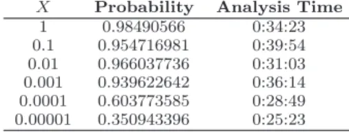
Table 1: Probability that fire is always smaller than X percent of the total area during 10000 seconds.
X Probability Analysis Time 1 0.98490566 0:34:23 0.1 0.954716981 0:39:54 0.01 0.966037736 0:31:03 0.001 0.939622642 0:36:14 0.0001 0.603773585 0:28:49 0.00001 0.350943396 0:25:23
As expected, the probability that the fire remains smaller than X% of the total area increases when X increases. In-deed, “the fire area remains smaller than X% of the total area” implies that “the fire area remains smaller than Y % of the total area” for any Y ≥ X. However, the probability returned is an approximation, with an error up to 0.1 with a confidence of 99%. Therefore, the fact that the probability decreases from 0.96 to 0.95 when X increases from 0.01 to 0.1 is not significant. Indeed, the difference between the two values is less than the error. On the contrary, the differ-ence between the probabilities obtained for X = 0.0001 and X = 0.001 are significant since they are more than twice the error. In our model, the total area is about 23 square kilo-meters. Therefore the two last lines of the table correspond to respectively an area of 23 and 2.3 square meters.
Table 2: Probability that fire area is smaller than X percent of the total area at least 90% of the time.
X Probability Analysis Time 1 0.954716981 00:40:05 0.1 0.981132075 00:34:25 0.01 0.966037736 00:43:22 0.001 0.977358491 00:42:37 0.0001 0,973584906 00:42:59 0.00001 0,996226415 00:37:25
In order to obtain the probability presented in Table 2, we subtract from 1 the probability that Pattern 2 holds. We obtain the probability that the fire is smaller than X percent of the total area for at least 90% of the time (over 10000s). Again, since for each value of X we ran a different set of simulations, it is not clear that the probability that the pattern holds increases when X increases. With this more permissive definition, we see that even small fires have a low probability to stay on for more that 10% of the simulation time. By comparing with Table 1, we can conclude that frequently occurring fires (i.e. very small ones) are quickly extinguished, because the probability of the last two lines are significantly higher in Table 2.
Finally, we evaluate the probability to obtain the un-wanted emergent behavior depicted in Figure 5, that is the probability that Pattern 3 holds. The returned result is 0.9622, which means that the probability that the contract holds is between 0.8622 and 1 with a confidence of 99%.
We showed here how our tool chain is used to evaluate whether a given pattern holds. By evaluating the probabil-ity of Pattern 1, 2 and 3, we were able to discover that small fire occur often (last two lines of Table 1) but are not likely to last long (last two lines of Table 2). Finally, the emer-gent behavior occurs with a probability between 0 and 0.14,
which explains why Pattern 1 and Pattern 2 do not occur with a probability of 1. This problem could be resolved by studying the causes of the emergent behavior and evolving the SoS to avoid it, for instance by adding more fire fighting cars.
At this level of analysis, a precision of 0.1 is sufficient to obtain a good general idea about the probability that each of the patterns occur. In general, using SMC requires to find the appropriate trade-off between the required preci-sion and the time available for the analysis and subsequent re-engineering.
Our Patterns are independent on the actual number of components. Indeed, adding constituent systems such as districts or cars, even if they have a new behavior, do not require specifying new patterns. The analysis is still possi-ble on the modified SoS model.
In the framework of the DANSE project, Industrial Part-ners built models of their SoS under analysis. SMC and other methods provided them a higher confidence in their models [4]. More precisely, one Partner verified Mean Time Between Failures (safety) requirements in an Air Traffic Con-trol case study. Another Partner verified sufficient water availability (robustness to failures) in a water distribution system of national scale.
6.
CONCLUSION, FUTURE WORK AND
RE-LATED WORK
This paper proposes a full tool-chain for the rigorous de-sign of Systems of Systems via formal reasoning and Statis-tical Model Checking.
Recent work promotes simulation techniques as the prin-cipal way to perform SoS analysis. In [38] the authors use discrete event specification (DEVS) concepts and tools to support virtual build and test of systems of systems. Their MS4-Me environment enables modeling and simulation (M&S) of SoS by allowing the user to specify constituent systems’ behavior in terms of a so-called Constrained Natural Lan-guage. The tool is implemented in Eclipse and employs Xtext, Eclipse Modeling Framework and the Graphical Mod-eling Project.
Recent work in [31] provides an overview of the under-lying theory, methods, and solutions in M&S of systems of systems, to better understand how modeling and simula-tion can support the Systems of Systems engineering pro-cess. However, simulation is an incomplete analysis and it is not able to assess the likelihood of the simulated behav-iors. This is not acceptable from the point of view of SoS analysis, as it does not provide to the designer sufficient confidence of correctness. Other approaches to verification of complex systems are based on exhaustive formal analysis, such as model checking, or simulation-based formal analy-sis, such as run-time monitoring. Industrial model check-ing techniques [8] are not adequate to the complexity and dynamicity of SoS. Run-time monitoring does not seem to be adequate to the context of SoS, where failures detection should provide a likelihood estimate of the failure and suffi-cient time for devising failure-avoidance corrections. In this perspective, a very promising approach to provide sufficient coverage of the SoS behavior while keeping the analysis cost low is based on Statistical Model Checking (SMC) [37]. SMC is a simulation-based formal analysis providing an estimate of the likelihood of requirement satisfaction and a tunable
level of confidence in the accuracy of analysis results. Some frameworks, such as BIP [7] or Reo [5] allow the user to describe architecture of systems using alternative composition operators. Both these frameworks theoretically permit composition of heterogeneous system, by including existing code into the components. However, they provide no standard such as FMI/FMU allowing to compile a par-ticular component independently of the architecture, which make them unsuitable for an industrial environment. They both include a stochastic extension [29, 28], which is not part of the core framework.
Contracts for reasoning about heterogeneous systems are presented in [24]. However, these contracts are considered at a very abstract level, and thus are not as useful as FMI/FMU from an industrial point of view.
Future Work.
Our objective is to improve our solution by exploiting rare-event techniques [21] that would allow us to detect rare emergent behaviors with a minimal amount of simulations. Our second future work is to automatize the relationship between the outcome of SMC and the reconfiguration pro-cess, in order to automatically find an architecture satisfying sufficiently the GCSL contracts.
7.
REFERENCES
[1] Speeds (2008): D2.5.4: Contract Specification Language. Public deliverable, Available at http://speeds.eu.com/downloads/D 2 5 4 RE Contract Specification Language.pdf, 2008. [2] Vv. Aa. D3.3.2 - Concept Alignment Example
description. Technical report, DANSE deliverable, 2013.
[3] Vv. Aa. D6.3.3 - GCSL Syntax, Semantics and Meta-model. Public deliverable, DANSE deliverable, 2015.
[4] Vv. Aa. DANSE Final Report. Technical report, DANSE deliverable, 2015.
[5] FARHAD ARBAB. Reo: a channel-based coordination model for component composition. Mathematical Structures in Computer Science, 14:329–366, 6 2004. [6] A. Arnold, B. Boyer, and A. Legay. Contracts and
behavioral patterns for sos: The EU IP DANSE approach. In K.G. Larsen, A. Legay, and U. Nyman, editors, Proc. 1st Workshop on Advances in Systems of Systems (AiSoS) 2013, volume 133 of EPTCS, pages 47–66, 2013.
[7] Ananda Basu, Marius Bozga, and Joseph Sifakis. Modeling heterogeneous real-time components in BIP. In Fourth IEEE International Conference on Software Engineering and Formal Methods (SEFM 2006), 11-15 September 2006, Pune, India, pages 3–12, 2006. [8] J.L. Boulanger. Industrial Use of Formal Methods.
John Wiley and Sons, 2012.
[9] B. Boyer, K. Corre, A. Legay, and S. Sedwards. Plasma lab: A flexible, distributable statistical model checking library. In QEST’13, pages 160–164, 2013. [10] D. Broman, C. Brooks, L. Greenberg, E.A. Lee,
M. Masin, S. Tripakis, and M. Wetter. Determinate composition of fmus for co-simulation. In Proc. of the 11th ACM Int. Conference on Embedded Software, EMSOFT ’13, pages 2:1–2:12. IEEE Press, 2013.
[11] Quentin Cappart, Christophe Limbr´ee, Pierre Schaus, Jean Quilbeuf, Louis-Marie Traonouez, and Axel Legay. Verification of interlocking systems using statistical model checking. submitted to IFM2016. [12] Alessio Colombo, Daniele Fontanelli, Axel Legay,
Luigi Palopoli, and Sean Sedwards. Efficient customisable dynamic motion planning for assistive robots in complex human environments. JAISE, 7(5):617–634, 2015.
[13] Alexandre David, Kim G. Larsen, Axel Legay, Marius Mikucionis, Danny Bøgsted Poulsen, and Sean Sedwards. Statistical model checking for biological systems. STTT, 17(3):351–367, 2015.
[14] D. Distefano, J.P. Katoen, and A. Rensink. On a temporal logic for object-based systems. In S.F. Smith and C.L. Talcott, editors, 4th International
Conference on Formal Methods for Open Object-Based Distributed Systems (FMOODS) 2000, volume 177 of IFIP Conference Proc., pages 305–325. Kluwer, 2000. [15] L. Mangeruca et al. D4.3 - DANSE Methodology V2.
Technical report, DANSE deliverable, 2013. [16] S. Flake and W. M¨uller. Past- and future-oriented
time-bounded temporal properties with OCL. In 2nd International Conference on Software Engineering and Formal Methods (SEFM 2004), pages 154–163. IEEE Computer Society, 2004.
[17] Klaus Havelund and Grigore Rosu. Synthesizing monitors for safety properties. In Tools and Algorithms for the Construction and Analysis of Systems, 8th International Conference, TACAS 2002, Held as Part of the Joint European Conference on Theory and Practice of Software, ETAPS 2002, Grenoble, France, April 8-12, 2002, Proceedings, pages 342–356, 2002. [18] T. H´erault, R. Lassaigne, F. Magniette, and
S. Peyronnet. Approximate Probabilistic Model Checking. In VMCAI, pages 73–84, 2004. [19] W. Hoeffding. Probability inequalities. J. of the
American Statistical Association, 58:13–30, 1963. [20] IBM. Rhapsody.
[21] Cyrille J´egourel, Axel Legay, and Sean Sedwards. Importance splitting for statistical model checking rare properties. In Computer Aided Verification - 25th International Conference, CAV 2013, Saint
Petersburg, Russia, July 13-19, 2013. Proceedings, pages 576–591, 2013.
[22] SumitK. Jha, EdmundM. Clarke, ChristopherJ. Langmead, Axel Legay, Andr´e Platzer, and Paolo Zuliani. A bayesian approach to model checking biological systems. In Pierpaolo Degano and Roberto Gorrieri, editors, Computational Methods in Systems Biology, volume 5688 of Lecture Notes in Computer Science, pages 218–234. Springer Berlin Heidelberg, 2009.
[23] S. Laplante, R. Lassaigne, F. Magniez, S. Peyronnet, and M. de Rougemont. Probabilistic abstraction for model checking: An approach based on property testing. ACM TCS, 8(4), 2007.
[24] ThiThieuHoa Le, Roberto Passerone, Uli Fahrenberg, and Axel Legay. A tag contract framework for heterogeneous systems. In Carlos Canal and Massimo Villari, editors, Advances in Service-Oriented and Cloud Computing, volume 393 of Communications in
Computer and Information Science, pages 204–217. Springer Berlin Heidelberg, 2013.
[25] Edward A Lee and Haiyang Zheng. Leveraging synchronous language principles for heterogeneous modeling and design of embedded systems. In Proceedings of the 7th ACM & IEEE international conference on Embedded software, pages 114–123. ACM, 2007.
[26] M.W. Maier. Architecting principles for systems-of-systems. Systems Engineering, 1(4):267–284, 1998.
[27] A. Mignogna, L. Mangeruca, B. Boyer, A. Legay, and A. Arnold. Sos contract verification using statistical model checking. In K.G. Larsen, A. Legay, and U. Nyman, editors, Proc. 1st Workshop on Advances in Systems of Systems (AiSoS) 2013, volume 133 of EPTCS, pages 67–83, 2013.
[28] Young-Joo Moon, Alexandra Silva, Christian Krause, and Farhad Arbab. A compositional model to reason about end-to-end qos in stochastic reo connectors. Science of Computer Programming, 80, Part A:3 – 24, 2014. Special section on foundations of coordination languages and software architectures (selected papers from FOCLASA’10), Special section - Brazilian Symposium on Programming Languages (SBLP 2010) and Special section on formal methods for industrial critical systems (Selected papers from FMICS’11). [29] Ayoub Nouri, Saddek Bensalem, Marius Bozga, Benoˆıt
Delahaye, Cyrille J´egourel, and Axel Legay. Statistical model checking qos properties of systems with SBIP. STTT, 17(2):171–185, 2015.
[30] A. Pnueli. The temporal logic of programs. In Proc. of the 18th Annual Symposium on Foundations of Computer Science, SFCS ’77, pages 46–57,
Washington, DC, USA, 1977. IEEE Computer Society. [31] L.B. Rainey and A. Tolk. Modeling and simulation
support for system of systems engineering applications. Wiley, Jan 2015.
[32] K. Sen, M. Viswanathan, and G. Agha. Statistical model checking of black-box probabilistic systems. In CAV, LNCS 3114, pages 202–215. Springer, 2004. [33] Vv.Aa. FMI standard specification. Modelica
association, https://www.fmi-standard.org/, 2012. [34] Vv.Aa. UPDM 2.0 formal specification. OMG,
http://www.omg.org/spec/UPDM/2.0/, 2012. [35] Vv.Aa. OCL language specification. OMG,
http://www.omg.org/spec/OCL/, 2014. [36] H.L.S. Younes. Verification and Planning for
Stochastic Processes with Asynchronous Events. PhD thesis, Carnegie Mellon, 2005.
[37] H.L.S. Younes and R.G. Simmons. Statistical probabilistic model checking with a focus on time-bounded properties. Inf. Comput., 204(9):1368–1409, 2006.
[38] B.P. Zeigler. Guide to Modeling and Simulation of Systems of Systems - User’s Reference. Springer Briefs in Computer Science. Springer, 2013.
[39] P. Ziemann and M. Gogolla. OCL extended with temporal logic. In M. Broy and A.V. Zamulin, editors, 5th Conference on Perspectives of Systems Informatics (PSI) 2003, volume 2890 of LNCS, pages 351–357. Springer, 2003.