Active versus passive fault-tolerant control of a redundant multirotor UAV

HAL Id: hal-02569240

https://hal.archives-ouvertes.fr/hal-02569240

Submitted on 11 May 2020

HAL is a multi-disciplinary open access

archive for the deposit and dissemination of

sci-entific research documents, whether they are

pub-lished or not. The documents may come from

teaching and research institutions in France or

abroad, or from public or private research centers.

L’archive ouverte pluridisciplinaire HAL, est

destinée au dépôt et à la diffusion de documents

scientifiques de niveau recherche, publiés ou non,

émanant des établissements d’enseignement et de

recherche français ou étrangers, des laboratoires

publics ou privés.

redundant multirotor UAV

Majd Saied, Benjamin Lussier, Isabelle Fantoni, Hassan Shraim, Clovis Francis

To cite this version:

Majd Saied, Benjamin Lussier, Isabelle Fantoni, Hassan Shraim, Clovis Francis. Active versus

pas-sive fault-tolerant control of a redundant multirotor UAV. Aeronautical Journal -New Series-, Royal

Aeronautical Society, 2019, 124 (1273), pp.385-408. �10.1017/aer.2019.149�. �hal-02569240�

Active versus Passive Fault-Tolerant Control of a

Redundant Multirotor UAV

M. Saied

, B. Lussier

, I. Fantoni

, H. Shraim

and C. Francis

Abstract

This paper considers actuator redundancy management for a redundant multirotor Unmanned Aerial Vehicle (UAV) under actuators failures. Different approaches are proposed: using robust control (passive fault tolerance), and reconfigurable control (active fault tolerance). The robust controller is designed using high order super-twisting sliding mode techniques, and handles the failures without requiring information from a Fault Detection scheme. The Active Fault-Tolerant Control (AFTC) is achieved through redistributing the control signals among the healthy actuators using reconfigurable multiplexing and pseudo-inverse control allocation. The Fault Detection and Isolation problem is also considered by proposing model-based and model free modules. The proposed techniques are all implemented on a coaxial octorotor UAV. Different experiments with different scenarios were conducted for the validation of the proposed strategies. Finally, advantages, disadvantages, application considerations and limitations of each method are examined through quantitative and qualitative studies.

NOMENCLATURE

X= [x y z]T Position vector w.r.t the inertial frame, m

Ω = [p q r]T _{Body axes Euler rates vector, rad/s}

uf Total thrust input, N

τ = [τφτθτψ]T Torque inputs vector, N.m

φ, θ, ψ Euler angles w.r.t the inertial frame, degrees

ωi Motor i speed, r pm

m Mass of the UAV, Kg

g Acceleration due to gravity, m/s2

Jr Propeller inertia, Kg.m2

e3 unit vector along the z axis

S(.) Skew symmetric operator

J= [Ixx, Iyy, Izz] Inertia matrix, Kg.m2

R Rotation matrix

Fi j Resultant thrust of two coaxial motors i and j

Fi Thrust produced by the motor i

τi Torque produced by the motor i

ωr Residual propeller speed, r pm

(.) Time derivative

I. Introduction

Over the last decades, the number of applications benefiting from unmanned aerial vehicles has increased considerably. Their introduction into the airspace leads to a number of safety issues. These include both safety issues on ground level to prevent

UAVs from falling and injuring people and/or damaging property, and safety issues in the air to prevent mid-air collisions.

Thus new generations of these vehicles must be designed to accomplish their work not only with high efficiency, but also

with increased safety and security. First, they are required to have an effective standardized collision avoidance system that

guarantees that the UAV can identify and be identified within the shared airspace and avoid risks to the surrounding traffic(1).

On the other hand, they should be equipped with fault-tolerant control systems (FTCSs) that enable the vehicle to continue operating correctly in the event of errors.

The implementation of fault tolerance requires redundancy in the system. An octorotor is an example of a multirotor UAV characterized by a built-in hardware redundancy, and will be taken as a case study in this paper. For a conventional quadrotor, complete loss of a rotor results in a vehicle that is not fully controllable. Partial failures of quadrotor actuators are investigated

in(2)_,(3) _{for system recovery and in}(4) _and(5) _{for fault detection and diagnosis. Up to three complete actuators failures are}

considered in(6) _{where relaxed hover solutions are proposed to allow a multirotor to maintain flight in spite of extreme centre}

of mass offsets while rotating at a constant velocity in hover.

1 _{Sorbonne Universit´es, Universit´e de Technologie de Compi`egne, UMR CNRS 7253 Heudiasyc, Compi`egne, France} 2 _{Lebanese University, Faculty of Engineering, Scientific Research Center in Engineering, Beirut, Lebanon}

Actuator redundancy available in an octorotor can be exploited, when an actuator fails, to re-allocate correctly the control effort among the healthy ones in order to retain complete controllability allowing the UAV to complete its mission.

The fault tolerant control of this type of vehicles has been recently studied and different strategies have been proposed:

Linear Parametric Varying (LPV) based sliding mode control allocation(7), neural network interval type-2 fuzzy sliding mode

controller(8), integral sliding mode scheme combined with fixed control allocation(9), cascade inverse method of control

allocation(10).

All the fault tolerant control papers cited above presented numerical simulations on an octorotor UAV in order to validate the proposed strategies.

This paper considers the problem of actuator redundancy management of a coaxial octorotor after failures resulting from

complete loss of actuator effectiveness. Its contribution is twofold. First, it extends our previous works presented in(11) and(12)

and validates in real flights three fault tolerant control architectures, two active and one passive, for a multirotor UAV:

• Active fault-tolerant control based on Inertial Measurement Unit for fault diagnosis and rule-based control mixing for

system recovery;

• Active fault-tolerant control based on motors speeds sensing for fault diagnosis and Pseudo-Inverse Control Allocation

for system recovery;

• Passive fault-tolerant control based on robust super-twisting sliding mode controller;

Second, the paper presents a comparative study of the proposed active and passive techniques from the viewpoint of technical, practical and theoretical performance. The main concern of this paper is to deal with some practical significant considerations in fault diagnosis and fault tolerant control of redundant multirotor UAVs such as tuning, complexity of design, real-time applicability, robustness, etc. It provides also an objective assessment of active and passive fault tolerant control methodologies applied on multirotor UAVs in a comparative setting. The comparison is carried out with real data from the Robotex coaxial

octorotor of the Heudiasyc Laboratory, France1.

The remainder of the paper is organized as follow. Section 2 presents the octorotor UAV: octorotor model, octorotor reconfigurability analysis and experimental platform. Section 3 presents the fault-tolerant control strategies: concepts, design and experimental results. These results are compared and discussed in section 4. Concluding remarks with future work are finally given in Section 5.

II. Octorotor UAV

The implementation of a FTCS requires the existence of redundancy in the system: hardware, software, information or time redundancy. An octorotor UAV has actuators redundancies, which make it an ideal system for FTC studies. We present in this section the equations of motion of the octorotor. A controllability analysis after actuators failures is investigated based on the distribution of the motors on the arms.

A. Octorotor Model

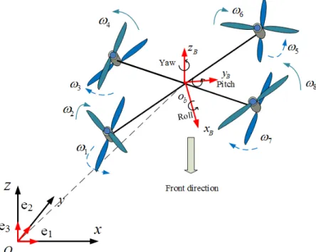
An octorotor UAV is a 6-Degrees Of Freedom (DOF) rigid body that consists in eight motors on which propellers are fixed

as shown in Fig. 1. They are attached at the ends of arms under a symmetric frame.

The state variables chosen to model the dynamics of the octorotor are the position and the altitude X = [x y z]T_{, in the}

inertial frame, the translational velocities ˙X, the Euler angles (φ, θ, ψ) and the angular velocitiesΩ = [p q r]T_{. The total thrust}

F= [0 0 uf]T, the roll, pitch and yaw torques τ= [τΦτθτψ]T are the virtual control inputs, while the motors speeds ωi,i=1...8 are

the real inputs. Using the Newton-Euler formalism, the nonlinear model of the octorotor UAV is obtained as follows:          m ¨X= −mge3+ RF ˙ R= RS(Ω) J ˙Ω + S(Ω)JΩ = τ (1)

S(.) is the skew-symmetric operator and J is the inertia matrix. The orientation of the octorotor with respect to the inertial

frame is represented by the rotation matrix R. The thrusts of the propellers are related to the virtual inputs as in (2) with Fi j

being the resultant thrust of two coaxial motors i and j(11) and τi the torque produced by the motor, Fi= kfω2_i and τi= ktω2_i:

               uf = F12+ F34+ F56+ F78 τφ= (F78+ F56− F34− F12)l √ 2/2 τθ= (F34+ F56− F78− F12)l √ 2/2 τψ= (τ2+ τ3+ τ6+ τ7) − (τ1+ τ4+ τ5+ τ8) (2)

The chosen platform for our experiments is the Modul-Air octorotor shown in Fig. 2 and built at Heudiasyc laboratory,

University of Technology of Compi`egne in France(13) shown in Fig. 1.b. Its parameters are given in(11). In the next sections,

passive and active FTCS will be tested on this octorotor. Only actuator failures are considered in this study due to their impact on the UAV stability.

Fig. 1: The coaxial counter-rotating octorotor and the reference frames

Fig. 2: The experimental Octorotor UAV

B. Reconfigurability Analysis

The analysis of the dynamics stabilization of a multirotor UAV starts with the definition of the necessary and sufficient

conditions for the system controllability and the control reconfigurability. An octorotor UAV is a nonlinear system with

positive control inputs since the rotors only provide a unidirectional thrust. Thus classical controllability theory(14) will have a

major limitation if applied to this system: the unilateral constraints do not pass the Kalman Rank Test. A slight modification of this test, however, can account for these constraints.

Consider a linear time invariant system written as:

˙x(t)= Ax(t) + Bu(t) (3)

with x(t) ∈ Rn_{. The rank condition for the controllability matrix M}

c= [ c1 c2 ... cm ]T = [ B AB ... An−1B ]T can

be expressed as:

Rank({α1c1+ α2c2+ ... + αmcm|α1, α2, ..., αm∈ R})= n (4)

To include the unilateral constraints, this condition is simply modified to a positive span,

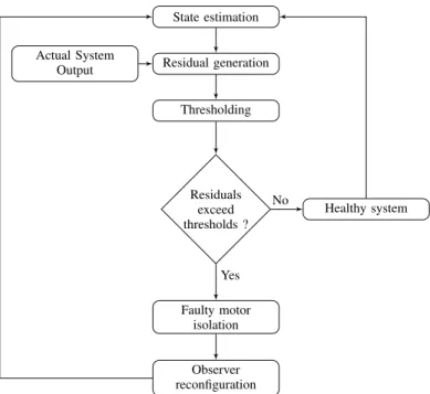
State estimation Residual generation Thresholding Actual System Output Residuals exceed thresholds ? Healthy system Faulty motor isolation Observer reconfiguration No Yes

Fig. 3: Fault detection and isolation algorithm

Considering the attitude system of the octorotor with x(t) = [φ ˙φ θ ˙θ ψ ˙ψ]T _{and u(t) = [ω}2

1ω 2 2... ω

2 8]

T_{, the application of the}

modified Kalman Test shows that the octorotor is not fully controllable when the two failed motors are not diagonally opposing

while rotating in the same direction or when they are coaxial motors(15)_.

III. Fault-Tolerant Control Strategies

Fault-tolerant control aims at ensuring that the system’s behavior stays correct despite the occurrence of faults and subsequent errors caused in the system. Generally speaking, fault tolerant control systems can be divided into two types: those that detect errors in the system and recovers from them (for example through reconfiguration or control allocation techniques) are known as active fault-tolerant control systems (AFTCSs), and those that tolerate faults without error detection (for example through robust control) are known as passive fault-tolerant control systems (PFTCSs).

A. Active Fault-Tolerant Control Design

An AFTCS typically consists of a Fault Detection and Diagnosis (FDD) scheme, a reconfigurable controller, a controller

reconfiguration mechanism and a command/reference governor(16). Based on this architecture, the design objectives of an

AFTCS are to design: (1) an FDD scheme with high sensitivity to faults that will not trigger false positive from model uncertainties and external disturbances; (2) a controller which can easily be reconfigured; (3) a reconfiguration mechanism which leads as much as possible to the recovery of the pre-fault system performance after failures occurrence, or at least to a degraded mode that ensures the safety of the system and its environment.

The critical issues in any AFTCS are the limited amount of time available for the FDD to detect and identify the error, the accuracy of the fault identification and the time taken to synthesize and deploy the new control schemes.

1) Design of fault detection modules: For this paper, we develop two different FDD modules for actuators failures: the first

one uses the Inertial Measurement Unit to detect uncontrolled movements of the UAV, the second one is based on the direct supervision of the motors speed and current.

a) Design of a model-based FDD: Model-based fault diagnosis is defined as the detection, isolation and identification

of faults from the comparison of a system available measurements, with a priori information represented by the system

mathematical model. Fault detection is supported by thresholding applied on residuals generated from the difference between

real and estimated measurements. A set of residuals must be designed, where each one is sensitive to a subset of faults. Model-based FDD comprises two main stages, residual generation and evaluation. For the octorotor case, residuals are generated using a nonlinear sliding mode observer, then they are evaluated according to the angles signature of each motor. The fault detection

and isolation strategy is illustrated in Fig.3.

Residual Generation: Residuals are constructed using Euler angles and their corresponding angular velocities. They are

functions of the difference between real and estimated outputs:

Real outputs yk are given by an Inertial Measurement Unit and estimated outputs ˆyk are deduced from a super-twisting sliding

mode observer whose equations are given below:

˙ˆx1= ˆx2+ z1 ˙ˆx2= f (t, x1, ˆx2, u) + z2 (7) with x1= [φ θ ψ]T, x2= [ ˙φ ˙θ ˙ψ]T and f =              Iyy−Izz Ixx ˙ θ ˙ψ − Jr Ixx ˙ θωr+_I1_xxτφ Izz−Ixx Iyy ˙ φ ˙ψ + Jr Iyy ˙ φωr+_I1_yyτθ Ixx−Iyy Izz ˙ φ˙θ + 1 Izzτψ              (8)

is the nonlinear part of the attitude model. Jr is the propeller inertia and ωr is the overall residual propeller speed from the

unbalanced rotors rotation:

ωr= ω2+ ω3+ ω6+ ω7−ω1−ω4−ω5−ω8 (9)

z1 and z2 are output injections given by the equations below using a low-pass filter(17):

z1= λ|x1− ˆx1|

1

2sign(x₁− ˆx₁)

z2= α sign(x1− ˆx1)

(10) α and λ are matrices of positive gains that guarantee the finite-time convergence of the observer.

Residual Evaluation: Residuals are examined for the verisimilitude of faults using thresholding method. According to (2) all

residuals are affected once a failure of any of the actuators occurs. The first time they go above the threshold level, the fault

is supposed to be present. A diagnosis inference model, based on the analysis of the failure modes, is presented in Table I(13),

and the algorithm in (11) is used to detect the failure of one motor.

f1 f2 f3 f4 f5 f6 f7 f8 ˙ φ + + + + - - - -˙ θ + + - - - - + + ˙ ψ - + + - - + +

-TABLE I: Diagnosis inference model for one rotor failure

if (ri> thresholdi)

{if ( ˙φ < 0 & ˙θ < 0 & ˙ψ < 0)} then motor 6 in failure

(11)

b) Design of a hybrid FDD: Model-free approaches rely on historical data collected from sensors and measurements,

without a need for a detailed mathematical model of the system. In this section, we present a combination of a model-based thresholding and a model-free classification where the fault diagnosis is carried out in two stages. The measured motor speed and the desired speed estimated from the control laws outputs are first compared. If they are not equal for a fixed amount of time, the motor is said to be failed. Its speeds and currents are then used as input data for a support vector machine block to

classify faults as propeller loss or motor failure. The FDD diagram is shown in Fig. 4.

DC Motor Modeling: The equations governing the operation of a Brushless Direct Current BLDC motor with speed ωMare

given below in Laplace transform:

I(s)=−KvωM(s)+V(s)

Ls+R

ωM(s)= KTI(s)−T_{J s+BM}L(s)

(12)

I, V, R and L are the armature current, voltage, resistance and inductance. Kvand KT are respectively the back-electromotive

and torque constants. Jr and BM represent the inertia of the rotor and the damping coefficient and TL the load torque. When

the motor stops rotating, i.e. ωM, the armature current, I(t)= V(t)/R, will reach the maximum value for a given input voltage

V. However, this is not true when simulating a motor failure, since we inject the fault by adjusting the motor’s voltage and

current to zero. With no propeller attached on the motor, the speed will increase with a decrease in the current (12). Support

Vector Machine (SVM): Support Vector Machines(18) _{are supervised learning models that can perform pattern recognition and}

classification problems. In this application, a SVM classifier is used to discriminate between propeller loss and motor failure.

Only two features are to be used: the electrical current and the speed of the motor. Different experiments were carried out to

collect these measurements before, during and after a propeller loss or a motor failure. The gathered data are trained using a C type SVM with a radial basis kernel.

Calculate |ωi−ωre fi| |ωi− ωre fi|> threshold Healthy motor wait∆t |ωi− ωre fi|> threshold SVM Type of Failure Finish No Yes No Yes

Fig. 4: Hybrid fault diagnosis diagram

c) Performance evaluation of both FDD techniques: Experimental Validation: The proposed FDD modules are validated

experimentally using fault injection. Failures on actuators 6 and 2 are simulated when the octorotor was hovering around

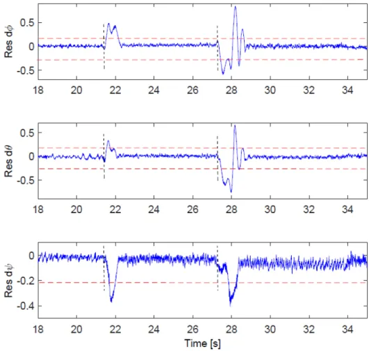
equilibrium. The position controller uses information from a motion capture system. For the first FDD module, figures5and6

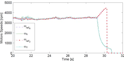
show respectively the residuals and orientation of the octorotor after the motors failures. The failures are injected respectively at times 21.37 s and 27.19 s, and isolated at times 21.65 s and 27.82 s, corresponding to detection delays of 0.28 s and 0.63 s. For the second FDD module, motors 6 and 2 are stopped simultaneously at time 29.18 s. The motor will no longer track

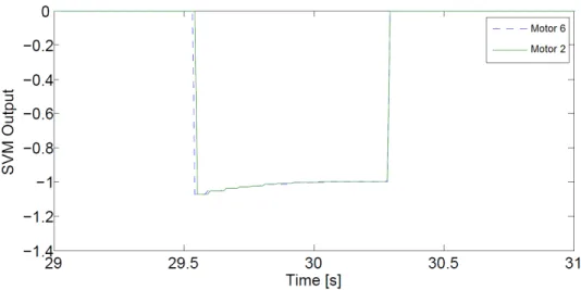
its reference speed as in Fig. 7 and the SVM prediction algorithm is triggered. Fig. 8 shows the variations of the armature

current and Fig. 9shows the SVM outputs (negative) corresponding to a motor failure. The detection delay is 0.36s.

Comparison: Generally speaking, it is not easy to compare fault detection schemes. The selection of a specific fault detection strategy depends upon several factors including characteristics of the process itself (linear or nonlinear, varying or time-invariant), the validity of the process model, and the application sensitivity. For critical applications, model-free approaches

are usually not recommended, as we have no guarantee that they will perform correctly in all situations(19)_{. Model-based}

approaches are preferred because their models and designs can be validated in the operation domain. In our case, we only used a model-free approach to distinguish between two types of faults. The fault detection and the failed component identification

were realized by a thresholding method, based on an electrical model of the motors, and are sufficient to perform system

recovery.

For the special case of an octorotor UAV, detecting motor or rotor faults directly using the motor controller offers several

advantages, as each motor can be considered as an auto-testable component:

• Only the motor/propeller model is necessary. The FDD module is then insensitive to the payload changes and the external

disturbances;

• It offers possibilities of detecting simultaneous faults since each motor is evaluated separately.

The main drawback of this method is the necessity of additional sensors to obtain motors information.

The proposed model-based FDD based on angle analysis makes use of the inertial measurement unit only, without need of any additional sensors. Although it shows good results during hovering flight after one or multiple successive failures, this model-based FDD is sensitive to external disturbances. In addition, it is not possible, using only the angular velocities, to isolate two or more simultaneous failures.

The performance criteria used to compare the two FDD methods are summarized in Table II.

Other performance criteria could be also used to compare the two FDD methods such as Diagnosis resolution and Error rate. The diagnosis resolution represents the average number of valid fault hypotheses per diagnosis, and the best possible value is 1. The error rate of a diagnosis system is defined as the average percentage of wrong diagnoses. An error rate of 0 is desirable. It is not easy to quantify these two variables in an experimental environment where parameters of both methods are

optimized in a way to reach the optimal point in the error rate/diagnostic resolution-plane, (0/1). However, according to the

previous comparison in terms of sensitivity to disturbances and uncertainties, one can deduce that the method based on motors information will probably be better in terms of error rate and diagnosis resolution, when considering missions specifications

Fig. 5: Residuals on angular velocities after consecutive motors failures.

Fig. 6: Euler angles after two consecutive motors failures.

different from what was considered during our experiments (for example aggressive maneuvers, outside flights), since these

specificities will have more effects on the system’s orientation than on the motors’ speeds and currents.

2) Design of system recovery techniques: We consider in this section two system recovery techniques: control allocation

and control mixing.

a) Design of a system recovery based on pseudo-inverse control allocation: The control allocation problem appears when

the controlled system has more physical actuators than control objectives(20)_{. Its design consists of several levels: (a) A high}

Fig. 7: Motors speeds and their references during hovering flight after two simultaneous motors failures.

Fig. 8: Motors currents during hovering flight after two simultaneous motors failures.

vector of these desired inputs into individual effector forces or moments. (c) A separate low-level controller to control the

actuators. For a multirotor UAV, four control objectives must be met (the thrust, the roll, pitch and yaw) using the available

actuators. After one or multiple actuator failures, the control effect can be re-allocated to the remaining working actuators by

the control allocation system without any need to reconfigure or re-design the controller. The pseudo-inverse is one the most used methods to solve unconstrained linear control allocation problems. Neglecting any constraints on the input, and giving

that τ= Bu, the control signal u is then written as:

u= [W−1BT(BW−1BT)−1]τ (13)

with W = diag{w1...w8} representing the effectiveness of the individual rotors and 0 < wi< 1. τ and u are defined previously.

The fixed matrix B is deduced from (2).

Angle Motor speed Analysis and current Quick detection and diagnosis √ √ Robustness to model uncertainties x √ Robustness to external disturbances x √ Low storage space and computation time √ √ Octorotor modeling requirement √ x Multiple successive fault identifiability √ √ Multiple simultaneous fault identifiability x √ Threshold identification √ √

Fig. 9: Diagnosis block output after two simultaneous motors failures.

b) Design of a system recovery based on offline rule-based control mixing: A nonlinear constrained optimization approach

is proposed to be used in order to calculate offline the solutions to a predefined set of failures and store them in a lookup

table. During the UAVs operation, the proper control mixing law is chosen according to the decision of the FDD module. This method presents the advantage of being facilely tested and validated before the first vehicle flight. The optimization problem is formulated as: minu1₂uTu such that: ( umin< u < umax Bu= τ (14)

with τ, B and u are as defined in the previous section. umax depends on the occurring failure. (6) is solved using the Matlab’s

multi-parametric programming tool. Based on the solution obtained, the control mixing gains are deduced for each failure case.

c) Performance Evaluation of the AFTCS: Performance Criteria: The following indices will be used for the performance

evaluation of the different FTCSs:

• The mean and maximum values of the tracking error;

• The settling time after fault injection;

• The control input energy;

• The practical applicability.

The reference tracking error is evaluated using the following measure:

e(t)= ||r(t) − yf tc||, (15)

where r(t) is the reference signal and yf tcis the system output with fault tolerance applied. Other performance indices can also

be used such as the mean and the maximum value of e(t), t ∈ [t1, t2], with t1 being the fault injection time, and t2 the settling

time of the control output with respect to the reference signal after the fault injection: ¯e=_t1 2−t1 Rt2 t1 e(t)dt emax= max t1≤t≤t2 {e(t)} (16)

For comparison, the longest settling time for a FTCS is selected for calculations.

The settling time is the time required for the state variables to return and remain within a range of certain percentage of their reference values. Since we are studying a real system response, we consider a percentage of 5% to determine the settling time.

The control input energy represents the mean value of energy of the control input signal u(t):

E=

Z ∞

−∞

|u2(t)|dt (17)

In all the tables below, the control input energy is evaluated only in the interval [t1, t2] defined previously.

Unlike the other indices presented above, which are quantitative, practical applicability is a qualitative performance criterion.

It consists of evaluating the possibility of real-time implementation and the difficulties that can be faced when a fault-tolerant

control strategy is applied on the system.

For the AFTCSs, an extra issue has to be considered: the time needed for the finalization of the controller reconfiguration after the fault occurrence. However, the uncertainty associated with the FDD decision will not be considered since we are

Fig. 10: Responses of pseudo-inverse control allocation under three different FDD delays

Fig. 11: Responses of reconfigurable rule-based control mixing under three different FDD delays

considering only complete actuator failures. Performance Evaluation: The evaluation of the AFTCSs is done under different

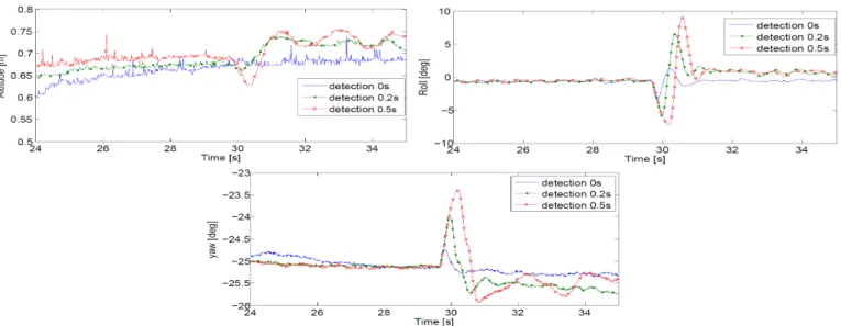
FDD time delays (0s, 0.2s and 0.5s). Since the response depends also on the fault injection time, all motors failures are injected once the UAV reaches the altitude reference and its attitude is stabilized around the equilibrium. Due to space limitations, only the responses in the roll (similar to the pitch response due to the system symmetry), the yaw and the altitude are illustrated

in Figures 10and11. Evidently, the performance of the multirotor deteriorates with the increase in FDD delays, assuming a

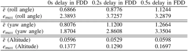
perfect fault estimation. The results of real time flights are summarized in Table IIIand TableIV. The AFTCSs without FDD

delay produce ¯e and emax of 0.6866 and 2.3893 using the reconfigurable control mixing method, and of 0.4717 and 2.8618

using the pseudo-inverse control allocation. Results are obviously worse with longer detection delays. B. Passive Fault-Tolerant Control Design

PFTCSs generally make use of only one robust controller, that deals with all the expected faults, without on-line fault information neither controller parameters reconfiguration. The main purpose is to develop a controller that makes the system insensitive to design basis faults. The critical issues in any PFTCS are first its reliability for the class of failures beyond design basis, and second the compromise between the nominal and the faulty performances. Note that a well known disadvantage of fault masking is that, as system errors are not detected, the fault masking can exceed its fault tolerance limit without warning, causing an unexpected failure of the whole system.

0s delay in FDD 0.2s delay in FDD 0.5s delay in FDD ¯e (roll angle) 0.4717 2.0360 2.5436 emax(roll angle) 2.8618 6.9843 9.4959

¯e (yaw angle) 0.1353 0.4220 0.5860 emax(yaw angle) 0.4007 1.1924 1.7765

¯e (Altitude) 0.0104 0.0404 0.0406 emax(Altitude) 0.0211 0.0694 0.0652

TABLE III: Performance indices of the AFTCS based on pseudo-inverse control allocation after one motor failure and under three time delays

0s delay in FDD 0.2s delay in FDD 0.5s delay in FDD ¯e (roll angle) 0.6866 0.8776 1.1244 emax(roll angle) 2.3893 3.7257 3.2879

¯e (yaw angle) 0.8076 1.1200 1.2664 emax(yaw angle) 1.8704 2.8608 3.3504

¯e (Altitude) 0.0596 0.0529 0.0598 emax(Altitude) 0.1377 0.1290 0.1697

TABLE IV: Performance indices of the AFTCS based on reconfigurable control mixing after one motor failure and under three time delays

1) Design of a PFTCS: Different passive FTC methods have been suggested in the literature, principally based on robust

theory, e.g. H∞, nonlinear regulation theory, Lyapunov and passivity-based FTC(21). It was proved in(9) that Sliding Mode

Control (SMC) has the ability to retain the desired performance without requiring fault detection and isolation. Sliding Mode

Control is a non linear robust state feedback control technique that uses switching control actions(22). It offers several advantages

in terms of low sensitivity to parameter uncertainties and external perturbations. This property makes it an excellent candidate for passive fault-tolerant control system.

The SMC presented here is based on the work introduced in(23)_{. It is a second order technique known as Super-Twisting}

Algorithm (STA). The design of this SMC for the coaxial octorotor starts by defining the state vector x: x1 = [z φ θ ψ]T,

x2 = [˙z ˙φ ˙θ ˙ψ]T and x= [x1x2]. The model describing the altitude and the attitude of the system is written as in (18) with

w(t)= [w1w2w3w4]T being the external disturbances vector:

(

˙x1= x2

˙x2= F(x) + G(x)u + w(t)

(18)

Different assumptions are considered: the state vector can be measured by sensors, the velocity and the acceleration of the

UAV are bounded and the aggressive behavior is not authorised. Under these constraints, the matrix is invertible, and the disturbances vector is bounded:

| ˙wi(t)| < δi (19)

The sliding surface is chosen as:

s= ˙e + λe (20)

with e= x1d− x1 and ˙e= x2d− x2 being the tracking errors, and λ is a positive definite matrix. The control that guarantees

that the system remains on the sliding surface can be found as: τ = G−1_{( ¨x} 1d−λ˙e − K1|s| 1 2sign(s) − K₂ Z t 0 sign(s(τ))dτ − f (x)) (21)

K1= diag(k11, k12, k13, k14) and K2= diag(k21, k22, k23, k24) are the gains matrices that verify:

K2i> δi

K_1i2 > 4K2i

i= 1, 2, 3, 4 (22)

The convergence proof is given in(23)_.

Normally, the main disadvantage of the sliding mode controller is the chattering: finite amplitude high-frequency oscillations of the controlled structure. However, the higher order sliding mode technique, which is a generalization of the first order sliding mode control with higher order derivatives of the sliding variable, reduces this undesirable phenomenon.

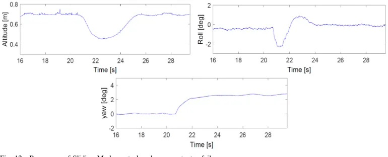
2) Performance evaluation of the PFTCS:: As for the AFTCS case, a failure on motor 6 is injected once the UAV reaches

its reference altitude. However, with PFTCS, no FDD nor controller reconfiguration delays need to be considered. The results

Fig. 12: Responses of Sliding-Mode control under one actuator failure

One Failure Two Failures ¯e (roll angle) 0.2674 0.8954 emax (roll angle) 1.8 2.666

¯e (yaw angle) 0.2520 2.8856 emax (yaw angle) 0.6 4.5

¯e (Altitude) 0.0991 0.1650 emax (Altitude) 0.1986 0.2420

TABLE V: Performance indices of the PFTCS based on robust SMC after one and two failures

IV. FTCSs Comparison Results

In the previous sections, the architectures of both active and passive FTCSs are introduced, and their performances are described. The experimental conditions of the system under AFTCS and PFTCS are chosen in a similar manner. Due to the design techniques used, some aspects of the results may be application-dependent. However, we believe that our general conclusions remain applicable.

In this study, the AFTCSs analysis assumes a precise diagnosis with a detection delay of 0.5s to focus the comparison on the recovery mechanisms. 0.5s is a rather pessimistic value for detection, guaranteeing under most circumstances a correct fault detection and identification. First, both approaches are designed under case 1: Failure of motor 6. Under this fault condition,

the Euler angles deviations resulting from the application of AFTCS and PFTCS are presented in Fig.13. It is observed that

the deviations in the AFTCSs cases have significant values when the reconfigurable controller or multiplexer are activated, which provokes considerable transients. In a PFTCS, the control surface deviations are much smoother, since it does not need to switch to a degraded mode. The performance of the AFTCS and PFTCS are evaluated considering the overshoot, settling

time, steady-state error, complexity design and tuning facility as illustrated in TableVI. Other criteria will also be considered

such as the applicability and control input energy. Table VI shows that the FTC scheme using the sliding mode controller

achieves better performances in terms of minimal overshoot, steady state error and settling time on the attitude. However, the input energy required by this controller is bigger than in the case of the tested AFTCSs. For the Pseudo-Inverse method, it is shown that using this technique, the steady state error remains greater than 5% of the reference value, and thus no settling

time is indicated in the table. The values of ¯e and emaxare calculated in the interval [t1, t2] where t2 is the longer settling time

for the other two techniques. In case of multiple failures, the performance of the robust controller degrades and AFTCSs are shown to be better. In practice, it is possible to tolerate up to four successive or simultaneous motors failures using AFTCS

but not more than two motors failures using PFTCS. Fig. 14 and Fig.15show that the AFTCS based on the reconfigurable

control mixing is better in terms of overshoot, settling time and steady-state error. A. Advantages and Limitations of AFTCS

Once a fault is detected, the AFTCS moves from the nominal mode to a different solution region to act against the fault and

reduce its effects. Within each of these regions, the optimal solution may exist with certain pre-determined performance criteria.

AFTC is less conservative than PFTC since the fault is treated as a scheduling variable and not an additional uncertainty against which robustness must be enforced. This is shown by the possibility of tolerating more faults using AFTCSs. For the special

Fig. 13: Comparison of responses of active and passive FTCS.

AFTCS: AFTCS: PFTCS: Reconf. Multiplexer Pseudo-Inverse CA SMC Overshoot (roll angle) (degrees) 3.2879 9.4959 1.9491 Overshoot (yaw angle) (degrees) 3.3504 1.7765 0.6 Overshoot (altitude) (m) 0.1697 0.0652 0.1986 Steady-state error (roll angle) (degrees) 1.1244 2.5436 0.9887 Steady-state error (yaw angle) (degrees) 1.2664 0.5860 0.2520 Steady-state error (altitude) (m) 0.0598 0.0406 0.0991 Settling time (roll angle) (s) 2.88 - 2.29 Settling time (yaw angle) (s) 5.41 - 1.07 Settling time (altitude) (s) 2.18 - 2.78 Time delay before control action 0.5 0.5 0 Complexity in design High High Low Control input energy Eroll 0.0191 0.0245 0.0432 TABLE VI: Performance comparison between active and a passive FTCS

Fig. 14: Euler angles [deg] after fault injection on motors 6 and 2 using Pseudo-Inverse Control Allocation;

case of an octorotor, during real applications, the PID controllers are the most used onboard UAVs since they present good performance and are easy to tune. In this context, the AFTCS scheme is able to provide fault tolerance to controllers that are not intrinsically fault tolerant.

The main limitation of an AFTCS is its high dependence on the FDD module outputs. Once an error occurs, no action can be performed until the fault is detected and diagnosed. The interval between the fault occurrence and its detection has a major

Fig. 15: Euler angles [deg] after fault injection on motors 6, 2, 8 and 4 using reconfigurable control mixing;

impact on the maintenance of the stability of the system. As illustrated in TablesIV,IIIand Figures11,10, the performance of

the system worsens with the increase in FDD time. The reconfigurable mixer or control allocation design depends heavily on

the output provided by the FDD scheme. Any wrong decisions in FDD can lead to loss of effectiveness in the system recovery.

In both of the presented AFTCS, the switching between the nominal and degraded modes leads to immoderate transients as

shown in Figures11,10and13. These transients, considered as shocks, can induce further damage in the system.

B. Advantages and Limitations of PFTCS

The main advantage of a PFTCS is its simple structure. Once designed, the controller does not change and no transients are caused by controller switching operation. The behavior of the system is much smoother than an AFTCS, as can be seen

in Fig. 13. Furthermore, as a fault masking technique, a PFTCS does not need a FDD scheme, thus there is no delay between

the fault and the recovery actions.

The robust controller is designed for both normal and post-fault system operation. Thus this solution cannot be optimum for all design scenarios. Moreover, the overall conservatism increases with the number of faults considered during the design stage. For an octorotor, no PFTCS can be found after more than two actuator failures and thus this method presents limited FTC capabilities. The main advantage of the PFTCS is the avoidance of the time delay required for FDD and control reconfiguration. However, by not detecting faults, successive failures may exceed the FTC capability without warning, causing unexpected failure of the whole system.

V. Conclusions

Although the development of fault-tolerant control strategies is the topic of many works in the multirotor UAVs community, some technical and real-time considerations in application to real multirotors are still missing. Rare are the studies that consider the design of methodologies that involve feasibility and real world requirements specifications.

This paper presents the design and real-time implementation of fault-tolerant control architectures for an octorotor under actuators failures. It deals with some practical considerations in fault diagnosis and fault-tolerant control for such systems including tuning, complexity of design, real-time applicability, etc.

In active FTC systems, both aspects, including fault detection and system recovery, are considered. The passive FTC system

capability is based on the robustness of a high order sliding mode controller. A comparative study between the different proposed

techniques, carried out from qualitative and quantitative perspectives, has been also presented in this paper and shows that

each technique has its own advantages and limitations. In general, active approaches are more flexible to deal with different

types of faults. However, they are highly dependent on the fault detection and identification accuracy and the detection delay. Passive FTC approaches are simpler to be implemented since they do not need neither an FDD scheme, nor a reconfiguration

mechanism. However, the main limitation of these approaches is that they can never be optimal for all design scenarios and the overall conservatism increases at the same time as the number of faults considered during the design phase, eventually restraining the set of possible tolerated faults. As a conclusion, the designer of the FTCS of a multirotor should select the appropriate method according to the targeted faults, their mean of detection and the probabilities of multiple failures.

Acknowledgements

This work was carried out and funded in the framework of the Labex MS2T (Reference ANR-11-IDEX-0004-02) and the ROBOTEX Equipment of Excellence (Reference ANR-10- EQPX-44). They were supported by the French Government, through the program “Investments for the future” managed by the National Agency for Research.

The authors would like to thank the Lebanese University research support program. References

[1] Mahjri, I., Dhraie, A. and Belghith, A. A Review on Collision Avoidance Systems for Unmanned Aerial Vehicles, International Workshop on Communication Technologies for Vehicles, 2015.

[2] Chamseddine, A., Zhang, Y., Rabbath, C.A., Join, C. and Theilliol, D. Flatness-Based Trajectory Planning/Replanning for a Quadrotor Unmanned Aerial Vehicle, IEEE Transactions on Aerospace and Electronic Systems, 2012, 48, (4), pp 2832-2848.

[3] Avram, R., Zhang, X. and Muse, J. Nonlinear Adaptive Fault-Tolerant Quadrotor Altitude and Attitude Tracking With Multiple Actuator Faults, IEEE Transactions on Control Systems Technology, 2018, 26, (2), pp 701-707.

[4] Avram, R., Zhang, X. and Muse, J. Quadrotor Actuator Fault Diagnosis and Accommodation Using Nonlinear Adaptive Estimators, IEEE Transactions on Control Systems Technology, 2017, 25, (6), pp 2219-2226.

[5] Chen, F., Jiang, R., Zhang, K., Jiang, B. and Tao, G. Robust Backstepping Sliding-Mode Control and Observer-Based Fault Estimation for a Quadrotor UAV, IEEE Transactions on Industrial Electronics, 2016, 63, (8), pp 5044-5056. [6] Mueller, M. and D’Andrea, R. Relaxed hover solutions for multicopters: application to algorithmic redundancy and novel

vehicles, The International Journal of Robotics Research, 2016, 35, (8), pp 873-889.

[7] Alwi, H. and Edwards, C. Sliding mode fault-tolerant control of an octorotor using linear parameter varying-based schemes, IET Control Theory and Applications, 2015, 9, (4), pp 618-636.

[8] Zeghlache, S., Saigaa, D. and Kara, K. Fault Tolerant Control based on neural network interval type-2 fuzzy sliding mode controller for octorotor UAV, Frontiers of Computer Science, 2016, 10, (4), pp 657-672.

[9] Alwi, H., Hamayun, M. and Edwards, C. An integral sliding mode fault tolerant control scheme for an octorotor using fixed control allocation, 13th International Workshop on Variable Structure Systems (VSS), 2014, pp 1-6.

[10] Marks, A., Whidborne, J.F. and Yamamoto, I. Control allocation for fault tolerant control of a VTOL octorotor, UKACC International Conference on Control, 2012, pp 357-362.

[11] Saied, M., Lussier, B., Fantoni, I., Francis, C. and Shraim, H. Fault Tolerant Control for Multiple Successive Failures

in an Octorotor: Architecture and Experiments, IEEE/RSJ International Conference on Intelligent Robots and Systems

(IROS), 2015, pp 40-45.

[12] Saied, M., Lussier, B., Fantoni, I., Shraim, H. and Francis, C. Passive Fault Tolerant Control of an Octorotor using Super-Twisting Algorithm: Theory and Experiments, 3rd Conference on Control and Fault-Tolerant Systems (SysTol), 2016, pp 361-366.

[13] Saied, M., Lussier, B., Fantoni, I., Francis, C., Shraim, H. and Sanahuja, G. Fault diagnosis and fault-tolerant control strategy for rotor failure in an octorotor, International Conference on Robotics and Automation (ICRA), 2015, pp 5266-5271.

[14] Sontag, E.D. Kalman’s controllability rank condition: From linear to nonlinear, Mathematical System Theory, Springer Berlin Heidelberg, 1991, pp 453-462.

[15] Saied, M., Shraim, H., Lussier, B., Fantoni, I. and Francis, C. Local controllability and attitude stabilization of multirotor UAVs: Validation on a coaxial octorotor, Robotics and Autonomous Systems, 2017, 91, pp 128-138.

[16] Zhang, Y. and Jiang, J. Bibliographical review on reconfigurable fault tolerant control systems, Annual Reviews in Control, 2008, 32, pp 229-252.

[17] Davila, J., Fridman, L. and Levant, A. Second-order sliding-mode observer for mechanical systems, IEEE Transactions On Automatic Control, 2005, 50, (11), pp 1785-1789.

[18] Vapnik, V. The Nature of Statistical Learning Theory, Springer, 2000.

[19] Sari, A.H. Data-Driven Design of Fault Diagnosis Systems: Nonlinear Multimode Processes, Springer Vieweg, 2013. [20] Boskovic, J. and Mehra, R. Control allocation in overactuated aircraft under position and rate limiting, American Control

Conference (ACC), 2002, pp 791-796.

[21] Benosman, M. Passive Fault Tolerant Control, Robust Control, Theory and Applications, InTech, 2011. [22] Edwards, C. and Spurgeon, S. Sliding Mode Control: Theory and Applications, Taylor & Francis, 1998.

[23] Derafa, L., Benallegue, A. and Fridman, L. Super twisting control algorithm for the attitude tracking of a four rotors UAV, Journal of the Franklin Institute, 2012, 349, (2), pp 685-699.