Chemical kinetics of SCRAMJET propulsion

Chemical Kinetics of SCRAMJET Propulsion

by

Rodger Joseph Biasca

S.B. Aeronautics and Astronautics, Massachusetts Institute of Technology, 1987 SUBMITTED IN PARTIAL FULFILLMENT OF THE

REQUIREMENTS FOR THE DEGREE OF

Master of Science in

Aeronautics and Astronautics

at the

Massachusetts Institute of Technology July 1988

©1988,

The author hereby grants to MIT and the Charles Stark Draper Laboratory, Inc. permission to reproduce and distribute copies of this thesis document in whole or in part.

Signature of Author

Department of Aeronautics and Astronautics July 1988 Certified by

Professor Jean F. Louis, Co- Thesis Supervisor Department of Aeronautics and Astronautics

Professor Manuel Martinez-Sanchez, Co- Thesis Supervisor pepartment of Aeronautics and Astronautics

nr Phillin T). Hattis, Technical Supervisor s Stark Draper Laboratory Accepted by

xtew, Ex3.*sh \. Professor Harold Y. Wachman, Chairman Department Graduate Committee

MAOHUSET1S r1nTSrn

OF TEO LOGY TH DRWN SEP 07 1988

Chemical Kinetics of SCRAMJET Propulsion by

Rodger Joseph Biasca

Submitted to the Department of Aeronautics and Astronautics

in partial fulfillment of the requirements for the degree of

Master of Science in Aeronautics and Astronautics

Recent interest in hypersonics has focused on the development of a single stage to orbit vehicle propelled by hydrogen fueled SCRAMJETs. Necessary for the design of such a vehicle is a thorough understanding of the chemical kinetic mechanism of hydrogen-air combustion and the possible effect this mechanism may have on the performance of the SCRAMJET propulsion system. This thesis investigates possible operational limits placed on a SCRAMJET powered vehicle by the chemical kinetics of the combustion mechanism and estimates the performance losses associated with chemical kinetic effects. The investigation is carried out through the numerical solution of one dimensional fluid flow equations coupled with the chemical kinetic expressions for the time rate of change of the fluid composition.

The results of the investigation show the hydrogen-air combustion process will place limitations on the pressure and temperature that must be maintained at the combustor entrance. For low initial pressures (P < 0.5 atm) and temperatures (T < 1000 K), the reactions become too slow for total heat release to be realized within a reasonable com-bustor length. In addition, hydrogen may fail to ignite for temperatures below 1000 K. Using a control volume method, it is shown that these required temperatures and pressures cannot be maintained over the entire trajectory for a vehicle with a fixed geometry.

In addition to the heat release problems, low pressures lead to substantial losses in nozzle performance. Low pressures mean third body reactions, the main path for recom-bination of free radicals, are inefficient. The dissociation energy in the flow exiting the combustor cannot be converted into kinetic energy in the nozzle. The nozzle freezes, leading to a drop in performance.

Finally, the specific impulse of the vehicle is shown to drop dramatically with decreas-ing combustor pressure. Best vehicle performance is achieved for flight at altitudes below the trajectories usually associated with hypersonic vehicles.

Thesis Co-supervisors: Jean F. Louis

Professor of Aeronautics and Astronautics

Manuel Martinez-Sanchez

Acknowledgements

Several days before the completion of this thesis, the life of Professor Jean Louis was tragically claimed in an auto accident. I dedicate this thesis to Professor Louis, whose guidance and encouragement have been so invaluable. The loss of Professor Louis is the loss of a good advisor and friend.

Many others have provided assistance in the course of writing this thesis. On this page, I only briefly mention a few and hope everyone understands my gratitude is more than can be expressed here. In particular, I would like to thank Professor Martinez-Sanchez, who has provided much of the direction of this thesis. Also, I owe a special debt of gratitude to Phil Hattis and Draper Laboratory for the foresight and financial support to pursue the topic of the once-again-fashionable hypersonic vehicle. On a more personal note, Mark Lewis, in addition to just being a good friend over the last year and a half, has provided a great deal of advice during my work on this thesis. Finally, I must thank my parents for 24 years of support and love.

OThis thesis was written under IR&D Task 236 of the Charles Stark Draper Laboratory, Inc. Publication of this thesis does not constitute approval by The Charles Stark Draper Laboratory, Inc. of the findings or conclusions contained herein.

Contents

Acknowledgements

1 Introduction

1.1 General Vehicle Configuration ...

1.2 Chemistry Models for SCRAMJET Analysis ... 1.3 Thesis Goals ...

2 Analysis

2.1 Inlet...

2.2 Quasi-One Dimensional Flow Equations ... 2.3 Finite Rate Chemistry ...

2.4 Equilibrium Flow ... 2.5 Numerical Solution.

3 Inlet Results

4 Static Reaction Results

4.0.1 Hydrogen-Air System .

4.0.2 Hydrogen-Air-Hydrogen Peroxide System. 4.0.3 Hydrogen-Air-Silane System .

5 Nozzle Results

6 Vehicle Performance Results 7 Conclusions

A Thermodynamic and Reaction Rate Data

1 7 7 8 11 12 12 14 17 19 26 28 32 32 38 38 45 57 66 71

List of Figures

1.1 General Configuration of a Hypersonic Vehicle. ... 8

2.1 Inlet at design conditions. ... 13

2.2 Inlet below design conditions. ... 13

2.3 Inlet above design conditions. ... 13

2.4 Model of the quasi-one-dimensional fluid element ... 15

3.1 Pressure and temperature delivered to the combustor for the first design point ... 29

3.2 Residence time per meter of a fluid element in the combustor assuming constant velocity (first design point). ... 29

3.3 Pressure and temperature of the flow delivered to the combustor for the second design point. ... 30

3.4 Residence time per meter in the combustor for the second design point. 30 4.1 Time history of the mass fractions in a stoichiometric hydrogen-air reaction with an initial temperature of 1000 K and an initial pressure of 1 atm. .. 34

4.2 Time history of the temperature in a stoichiometric hydrogen-air reaction with an initial temperature of 1000 K and an initial pressure of 1 atm. .. 34

4.3 Total reaction times for the H2-Air system as a function of initial tem-perature and pressure. . . . ... 35

4.4 Effect of equivalence ratio on the H2-Air reaction. 36 4.5 Required lengths of the combustor at the first design point for complete combustion to occur. ... ... 37

4.6 Required lengths of the combustor at the second design point for complete combustion to occur. ... 37

4.7 Total reaction times for the H2-air-2.5% H202 system as a function of initial temperature and pressure . . . ... 39

4.8 The effect of increased mass fraction of H202 on the total reaction time for various initial temperatures and pressure ...

4.9 Effect of hydrogen peroxide as a function of temperature for T< 1050 K. 4.10 Total reaction times for the H2-Air-2.5% mass fraction SiH4 system as a

function of initial temperature and pressure ... 4.11 Effect of increasing SillH4 on the reaction time ...

4.12 Total reaction times for mixtures containing 5% and 10% mass fraction silane as a function of temperature and pressure ...

4.13 The effect of 5% silane on the lengths required for total combustion. Design point 1 ...

4.14 The effect of 5% silane on the lengths required for total combustion. Design point 2 ...

4.15 The effect of 10% silane on the lengths required for total combustion. Design point 2 ...

5.1 , vs initial pressure and temperature for an initial velocity of 5500 m/s and 12.5 degree half angle conical expansion ...

5.2 r as a function of pressure and temperature for an initial velocity of 5500 m /s . . . . .. . . . ... . . . . 5.3 ¢ as a function of pressure and temperature for an initial velocity of 5500

5.4 5.5 5.6 5.7 5.8 5.9 5.10 5.11 5.12 6.1 6.2 6.3 6.4 6.5

m/s. o..

..o.. o

...

The effect of area ratio on ... The effect of area ratio on C . . The effect of nozzle half angle on . The effect of nozzle half angle on .. The effect of nozzle half angle on C.

Specific impulse vs. Mach number and altitude for the first design point. Specific impulse vs. Mach number and altitude for the second design point. Penalty for kinetic solution for first design point . ...

Penalty if nozzle were completely frozen for second design point .... Penalty for kinetic solution for second design point . ...

39 40 41 41 42 43 44 44 46 46

... ...47

... . ..49

... . ..49

... .... . 50

... . ..52

... . ..52

... . ..53

... . ..55

... . ..56

6.6 Penalty if nozzle were completely frozen for first design point. ... 62 6.7 Specific impulse vs. equivalance ratio for various flight conditions.

De-sign point 1. ... 63

6.8 Specific impulse vs. equivalance ratio for various flight conditions. Design

List of Tables

2.1 Influence Coefficients with Chemistry Added: Fuel and Area. ... 20 2.2 Influence Coefficients with Chemistry Added: Fuel and Pressure ... 20 2.3 Influence Coefficients with Chemistry Added: Fuel and Temperature. .. 20

5.1 Numbering system of lines ... ... 48

A.1 Polynomial curvefit coefficients for the enthalpy of individual chemical species in thermal equilibrium as a function of temperature ... 72 A.2 Polynomial curvefit coefficients for the enthalpy of individual chemical

species in thermal equilibrium as a function of temperature (con't)... 73 A.3 Reaction mechanism for the H2-Air system and values of the constants

for the Arrenhius expression. ... 74

A.4 Third body efficiency factors for the H2-air system ... 75 A.5 Silane reaction mechanism and values of the Arrenhius expression

Chapter 1

Introduction

In 1986 a new national effort began to develop a hypersonic aircraft: interest in hyper-sonics is once again growing after having lain nearly dormant since the cancellation of the X-15 project in 1968.

Several possible missions exist for such a hypersonic aircraft. The aircraft considered here is a single stage to orbit vehicle capable of horizontal take- off and landing and propelled throughout the flight exclusively by air- breathing engines.

1.1 General Vehicle Configuration

Figure 1.1 shows the general configuration of the hypersonic vehicle most prevalent in the current literature (see for example References [1], [2] and [3]). Since no single air-breathing propulsion system is capable of providing efficient thrust across the entire trajectory from take-off (Mach number, M=O) to orbital velocity (M=25), the airbreath-ing engines must actually consist of several propulsive modes. From takeoff to M=3, conventional turbojets provide efficient thrust. Above approximately M=3, however, the efficiency of the turbojet begins to drop as large total pressure losses are accrued in the turbomachinery. Such components as the compressor must be removed from the flow path.

With the turbomachinery removed from the flow path, the engine becomes a ramjet. In the ramjet, a series of shocks compresses the incoming flow to subsonic velocities. Fuel is then combusted in the subsonic stream, and the flow re-expanded through a nozzle.

Above Mach 6, the shocks required to decelerate the flow to a subsonic velocity become quite strong, again causing large total pressure losses. For high Mach numbers, the flow is not decelerated to subsonic velocities. Instead, the fuel is combusted in a supersonic airstream. The engine becomes a supersonic combustion ramjet, or SCRAMJET.

inletlforebody

SCRAMET

Figure 1.1: General Configuration of a Hypersonic Vehicle. The entire undersurface of the aircraft is integral to the propulsion system with the forebody acting as an inlet and the aftbody playing the role of a nozzle.

performance along the trajectory, the concern of this thesis is strictly limited to the chem-ical kinetic processes occurring in the SCRAMJET. With this in mind, the turbojet and ramjet modes will not be discussed further.

The figure shows the vehicle in the SCRAMJET propulsion mode. In this configuration, in order to increase thrust to weight ratios, the entire undersurface of the vehicle is integrated into the propulsion system. The forebody of the aircraft also acts as the engine inlet by providing a series of ramps to generate oblique shocks through which the incoming air is compressed. The compressed flow then enters the SCRAMJETs which act as the combustion chamber for the overall engine. Finally, the flow re-expands across the aftbody of the aircraft, which acts as the nozzle.

1.2 Chemistry Models for SCRAMJET Analysis

A single stage to orbit vehicle will encounter vastly varying flight regimes over its tra-jectory. Unfortunately, many of the conditions to be encountered are outside the range of conventional wind tunnel facilities. Without the conventional tool of the wind tunnel test, the aircraft's designers will need to rely heavily on computational fluid dynamics (CFD) to provide the analysis necessary for design.

In order to provide true performance estimates, the CFD codes need to solve the full 3-D Navier-Stokes equations. Integral to the success of these calculations is also the use of an accurate chemistry model. Unfortunately, even with the largest computers, calcula-tions incorporating the most accurate (and most complex) chemistry models are presently

-computationally and economically prohibitive. In addition, such solutions cannot easily be generalized to provide physical insight into the mechanisms affecting the performance of the vehicle. For preliminary designs, however, the calculations can be greatly simplified by hypothesizing simplified chemical models that adequately reproduce the true chemical effects.

Several chemical models of varying levels of complexity can be constructed: * Perfect Gas

In this model, the flow consists of a hypothetical perfect gas of constant composition and specific heat. Although quite simple, the model is inappropriate for situations above approximately 1200 K for air. Above this temperature, dissociation of oxygen changes both the chemical composition and specific heat of the gas. In addition, the model is obviously not suitable for combustion calculations where changing composition is the most important consideration.

e Frozen Gas

Here, the composition of the gas is constant, but the specific heat varies as a function of temperature. Although an improvement over the perfect gas model in some situations, the frozen gas model is still limited to situations where the chemical composition of the gas is slowly varying.

* Equilibrium Gas

In this model, the flow is assumed to be in chemical equilibrium at every point in the flow. This assumption allows the chemical composition of the flow to be determined from other thermodynamic variables such as pressure and temperature. Unfortunately, the determination of the chemical composition requires solving a set of nonlinear algebraic equations, a task that greatly increases the cost of computation over the previous models. In some situations, however, the equilibrium assumption can provide an adequate model of combustion without the additional complications introduced by the finite rate case discussed below. The equilibrium model fails when the characteristic times associated with the chemical reactions become of the same order as the characteristic time of the flow properties.

* Finite rate chemistry

Finite rate chemistry models integrate the expressions for the time rate of change of the chemical composition of the gas. Although providing "real" estimates of

the chemistry that is occurring, the model introduces widely varying times scales into the problem, i.e. the governing equations become quite stiff. The stiffness of the equations requires sophisticated techniques for efficient integration. Even then, integration of complete reaction mechanisms taxes the largest computers.

Since the integration of the stiff equations again reaches the point of being com-putationally prohibitive, a subclass of "two step global reaction models" has been developed. As an example, for the combustion of H2 in air, the complete reaction mechanism consists of approximately 60 reactions among 20 species. Many of these reactions and species are unimportant and can be ignored with negligible error. In the two step global model, the reaction mechanism is replaced by two hypothetical reaction paths among five species. The accurate reproduction of the true chemistry then requires the determination of the hypothetical reaction rates over a desired range of temperature and pressure. Several of these models have been developed in the literature.

e Finite rate chemistry with multiple modes of nonequilibrium

The models above have only considered chemical nonequilibrium. However, in some situations, rotational and vibrational nonequilibrium may also exist. For the most accurate calculations, these modes should also be included in the rate calculations. Since further time scales are introduced, these calculations are usually beyond the capability of even the most sophisticated computer systems. Fortunately, however, since the characteristic relaxation times for the rotational and vibrational modes are usually much faster than the chemical time scales involved, equilibrium assumptions are usually adequate.

Most CFD codes presently in use for combustion calculations use either an equilibrium assumption or a two-step global reaction mechanism. Before applying these models, however, the designer must have a reasonable concept of the effect the assumption may have on the final solution.

1.3 Thesis Goals

The purpose of this thesis is to investigate the effect of finite rate chemistry on a SCRAM-JET. The investigation includes

* predicting operational limits of the vehicle dictated by the kinetics of the combustion process, and

* estimating the performance losses incurred from the chemistry.

In order to evaluate the effect of finite rate chemistry, the complete reaction mechanism must be considered. As mentioned above, a three- or even two- dimensional solution with the complete reaction mechanism requires extensive computing facilities. In order to retain the full reaction mechanism, this thesis will only consider quasi-one-dimensional flow. The restriction to quasi-one- dimension reduces the partial differential equations to ordinary differential equations, a great simplification since efficient methods exist to integrate large sets of coupled, stiff ODEs. Although clearly not quantitatively correct in areas of complicated geometry, the model does provide insight into the effects of the finite rate chemistry and shows where simpler models may be inadequate.

In keeping with the simplicity of the quasi-one-dimension assumption, and in order to retain the emphasis on the effects of the chemical kinetics, several other major effects will be ignored. The major further assumptions are that

* the flow is inviscid, * heat losses are negligible,

* the fuel mixes instantaneously with the core flow in the engine.

The thesis is divided into seven chapters. Chapter 2 develops the analytic models of equilibrium and finite rate flow. In addition, a model of the inlet is included that is used to relate the combustor properties to the freestream flight conditions. The results of this inlet model are discussed in Chapter 3. Chapter 4 states the results of a static chemistry model. The static reaction model provides a way of easily investigating the operational limits placed on the vehicle by the combustion process. Chapter 5 presents the results for the vehicle nozzle and discusses the performance losses incurred from freezing in the nozzle. Chapter 6 presents the overall performance estimates of the propulsion system. Chapter 7 states the conclusions of the study.

Chapter 2

Analysis

The first section of this chapter develops a control volume method for the analysis of the engine inlet. Although the main focus of the thesis is the combustor and nozzle, the inlet analysis is required so the freestream flight conditions may be related to the initial conditions of the combustor/nozzle analysis. Following the inlet analysis, the governing equations for quasi-one-dimensional flow are stated, and the equations of the finite rate chemistry model derived. A section is also devoted to discussing the solution for equilibrium flow. The equilibrium flow solution is useful for comparative purposes with the finite rate case. The chapter concludes with short discussions on the numerical techniques used to integrate the equations.

2.1 Inlet

In order to relate the conditions at the beginning of the combustor to the freestream flight conditions, a model is needed for the inlet. For this thesis, the inlet consists of two ramps of equal turning angle. Figure 2.1 shows the general configuration of the inlet at the design conditions. At design, the shocks generated from the forward ramps intersect at the cowl lip. The cowl lip then reflects the shocks which are cancelled at the upper wall. A settling duct damps nonuniformities before the flow reaches the beginning of the combustor.

For a given design Mach number and ramp angle, the requirement that the shocks intersect at the cowl lip and are cancelled at the upper wall completely determines the geometry of the inlet. For flight off the design condition, the shocks no longer reflect from the cowl at the correct angle to be cancelled at the upper wall. As the vehicle moves below the design Mach number, the shocks move forward, missing the cowl (see Figure 2.2). At Mach numbers above the design condition (see Figure 2.3), the shocks intersect before reaching the cowl. They then enter the settling duct and weaken through a series

a -

--a -

-* -

-:.... . ... .... -. ' . . - :...

control volume

Figure 2.1: Inlet at design conditions. The shocks intersect at the cowl lip and are cancelled at the upper wall.

i -- .- ---... -.

-_a ,~ ' - .. " -.

- ~ ~ ~ ~ .s _

Figure 2.2: Inlet below design conditions. The shocks move forward missing the cowl lip. The shock generated from the cowl then intersects the upper wall, reflects, and begins a series of interactions with an expansion fan. m.-. ... ! a- -. _

Figure 2.3: Inlet above design conditions. The shocks intersect before reaching the cowl, reflect from the cowl, and begin a series of interactions with the expansion fan.

of reflections.

With the geometry of the inlet determined for a given design Mach number and ramp angle, the global conservation equations can be solved to find the values of the flow properties at the beginning of the combustor. Denoting freestream conditions by the subscript '0' and conditions at the beginning of the combustor by the subscript 'e', the conservation equations for the control volumes shown in Figures 2.1 to 2.3 are

* Mass

pouoAo = Pe Ue Ae (2.1) * Momentum

PO u A (ue - UO) = Pi Ai cos Oi (2.2) where the summation is taken over the sides of the control volume and Oi is the local inclination of the wall to the freestream velocity vector.

* Energy

ho + u/2 = he + u2/2 (2.3)

* State

P = pRT

(2.4)

The assumption is made that the gas is in equilibrium at point e. The enthalpy of the gas is then a function of pressure and temperature (the solution of the equilibrium composition is discussed in Section 2.4). Since the geometry is known from the design conditions,

global conservation provides four equations for the four unknowns (Pe, u, Pe, Te) at the combustor entrance. The solution of these four equations provides the conditions at the combustor entrance for any flight conditions.

2.2 Quasi-One Dimensional Flow Equations

This sections develops the equations of quasi-one-dimensional flow. The development follows closely the classical 'Influence Coefficient' method derived by Shapiro [4]. Figure 2.4 shows a differential element of gas of length dx travelling at a velocity, V, in the x-direction along a channel of cross sectional height, A. The fluid properties of interest are the pressure, P, temperature, T, density, p, enthalpy, h, and molecular weight, w. The fuel fraction, f, is defined as

A+dA

A :

iP

Figure 2.4: Model of the quasi-one-dimensional fluid element showing the change in fluid properties in the x-direction.

Mass is being injected into the stream at rate Mni df, energy is being added at a rate of dQ, and work is being done on external bodies at rate dW. In addition, a frictional force given by r, dA,, , where r, is the shear stress and dA, is the wetted surface area of the differential element acts on the fluid.

For this element of fluid, the governing equations in differential form for quasi-one dimensional flow are

* State: dP dp dw dT

P

p+

+T

(2.6)

P

p

w

T

+

(2.7)

dP

dV

+ Cf, dA +

df

(2.8)

V

2A

+

f

+df

where the shear stress -r has been expressed in terms of the friction coefficient, Cf. Also, the term hT represents the change in the total enthalpy of the injected gas between the wall temperature and the flow temperature, i.e. hT = (h + V2/2)T - (h + V2/2),,,, .

To find expressions for h and w, the fluid is considered to be a mixture of gases containing n molecular species, each of crj moles per kilogram flow. In addition, the

individual species are assumed to be in thermal equilibrium. (For justification of this assumption, the reader is referred to Vincenti and Kruger[5], where it is shown that rotational equilibrium will be reached within a few mean free paths of a strong shock. Comparison of the Landau-Teller model also shows the relaxation time for vibrational equilibrium to be much shorter than the chemical relaxation times for the gas of interest. Further information about the relaxation times for vibration can be found in the paper by Bussing [6]. )

For individual chemical species in thermal equilibrium, the enthalpy must be a function of temperature alone, i.e. h = h(T) [7]. The enthalpy as a function of temperature may be found from either the partition function or, more practically, polynomial curvefits derived from the partition functions. Excellent sets of these curvefits may be found in References [8], [9], and [10].

Since enthalpy is an extensive property, the enthalpy of the mixture is simply the sum of the enthalpies of the individual species:

ns

h =

h

j=l where h is the enthalpy of the j th species.

In addition, the molecular weight of the mixture is

W ,1 (2.11)

j=l j

The method for determining the values of the oj's will be discussed later for both finite rate and equilibrium flow.

Expressions are also assumed to be available for friction coefficient, work load, and heat losses (e.g. from boundary layer solutions). Although, as pointed out in the introduction, these terms will be considered negligible (Cf=dQ=dW=0), they will be retained for the sake of completeness throughout the algebraic development of the next few pages.

Equations (2.6) - (2.9) provide four equations for eight variables (dP, dp, dw, dT, dV, dA, dh, and df). As mentioned above, the dh and dw terms may be found in terms of the other variables by using an appropriate gas model. The solution of the problem then only requires specifying two of the remaining six variables as independent functions of x.

In the development of the influence coefficient method, Shapiro introduces the relations for Mach number, M, and ratio of specific heats, y, and then solves the above equations to provide a set of coefficients relating the dependent variables, dM2

dV dT and dp to

MT, 71f a- P such independent variables as dA _{such idpne} d _{v a} d ,and d-y The coefficients derived are functions_{s -- I}

of only the Mach number and the ratio of specific heats. Such a development is sufficient for perfect gases in which the Mach number and a are well defined. However for a flow in which chemical reactions are occuring, both Mach number and 7 lose meaning. Since the main focus of the work here is to study the effect of chemical reactions, M and are not introduced and the development of the equations is continued in terms of the primitive variables (P, T, V, h, etc).

2.3 Finite Rate Chemistry

This section develops the finite rate chemistry model following closely the development of Reference [11]. The fluid again is considered to be a gas mixture of n species with molar-mass concentrations aj . Between these chemical species, the chemical reactions are written in general as

ns ns

1Vij =

viisj

j=l j=l

where sj represent the chemical species, vij represents the stoichiometric coefficient of the jth species in the ith reaction, and nr is the number of reactions.

The forward production rate for a single reaction is ns

Rf,i = kf,i J (pa)'j i = 1,nr (2.13)

j=1

where the forward rate constant, kf,j, is given by the Arrhenius formula

kf,i = Ai Tni exp(-Bi/RT) (2.14)

where Ai is the rate constant of reaction i, n is an exponent, and B is the activation energy for the reaction.

Likewise, the expression for the backward rate constant is ns

Rb,i = kb,i

II

The forward and backward rate constants can also be related through

kb,i = kfi (2.16)

The net production rate of species j is the difference between the forward and backward rates of production, namely

dIjr ( v

Vdo

=r

kfK-,i

'

(po))

1-

j

+

du

(2.17)

~dt

P

f~[l

I

dt

i=1 t9

1

where -jt represents an external source term of species j to account for mass addition to the flow.

Several of the reactions in the H2-air reaction mechanism involve third bodies, M. In these reactions, any chemical species may act as the third body. The molar-mass fraction of the third body in reaction i is defined as

ns

rM,i = mijrj (2.18)

j=1

where mi,j is an 'efficiency factor' of the jth species in reaction i.

Equation (2.17) now provides a means of expressing the differential forms of Equations (2.10) and (2.11). For differentiation with respect to x:

d n

aj

d

dT

1

j=1 j=1

and

dw -1 ns daj(2.20

dx V(j(Es 1 Oj)2 dx

Equations (2.19) and (2.20) can now be combined with Equations (2.6)-(2.11). Tables (2.1)-(2.3) present the solution of these flow equations in a manner analogous to the influence coefficients of Shapiro. Each table shows the dependence of the derivative in the left most column on the derivatives in the upper row, e.g.

dP

M7-I

dA

M ( - 2 - 1) df +

(221)

P 7-(l-M)-1

A

(1-M)+ 1 +f *

pV

P

P

n3

-=

aj

,

T

(2.24)

where dQ and dW are again the heat added to and work done by the fluid element, respectively.

The three tables show the coefficients for different independent variables. The inde-pendent variables in the tables are, respectively,

* Fuel fraction and Area * Fuel fraction and Pressure * Fuel fraction and Temperature

The solution of the flow equations requires simultaneously integrating the expressions shown in the tables with the species conservation equations of Equation (2.17).

2.4

Equilibrium Flow

An equilibrium flow solution is useful for comparison with the results of the finite rate case. This section develops the equations for equilibrium flow. The development is modelled after that of Reference [12]

If the gas mixture containing ns species is ultimately comprised of n, elements, each of the species may be expressed from a set of stoichiometric coefficients aij , such that aij gives the number of i atoms present in mole species j. The total number of atoms of each element per unit mass of the mixture, b , can be found from the mass balance

ns

b0 = aijaj i = 1,ne (2.27) j=l

If the gas is in equilibrium, all thermodynamic properties of the gas are specified if two thermodynamic properties and the atomic composition (specified by knowing b ) are known. Throughout this work, the most convenient thermodynamic variables are

Table 2.1: Influence Coefficients with Chemistry Added: Fuel and Area. The derivatives in the left most row are related to the derivatives in the upper column through the given coefficients.

Table 2.2: Influence Coefficients with Chemistry Added: Fuel and Pressure.The derivatives in the left most row are related to the derivatives in the upper column through the given coefficients.

a.';l h d - dp dP Ž= 3 1 dW Cf l+f dW 1a.COT

W

-1,

_7-

_.

Table 2.3: Influence Coefficients with Chemistry Added: Fuel and Temperature. The derivatives in the left most row are related to the derivatives in the upper column through the given coefficients.

E'I h dj - d W Cf

dT df Ži=1h dW C dA

P

EM

M (: - 1)

-E.M

0

-M

A

1 +

- M) 1 + M + C(1 -M)

7(1

-M)

-1

M

pressure and temperature. With this functional dependence of h=h(P,T,bi) in mind, the differentiation of Equations (2.10) and (2.11) yields

Oh Oh n" Oh

dh

= ()dT

+

(-P

)dP + E(-

)dbi

and

d w = (W )dT + (-p) dP + E (a ) dbi /=1

Expanding Equations (2.10) and (2.11) and substituting intc (2.29), no OhQ h n&o

dh

=

(E

a

+

E

h )dT

+ (E h

j=1Tl

T

+

Z( Z

ho

0

'

)

db

-1

(Z)

dT+

aL

eP

ai

)

dj

)d

where the equilibrium values of rj and the partial derivatives have yet to be found as functions of P, T and b0.

First, to find the values of aj , the requirements for a gas to be in equilibrium are considered. Since the specified variables are pressure and temperature, the proper requirement for equilibrium is the minimization of the Gibb's free energy. For the mixture of gases, the free energy is [5]

(2.32) g = E Pj aj

j=1

where j is the chemical potential defined as

ag

-J

=

(D4

(2.33)

Equilibrium requires the minimization of Equation (2.32) subject to the mass constraint of Equation (2.27). Introducing the Lagrange multipliers, Ai, gives the following:

ne ns

G g +Z Ai(Z aiaj - b) = 0

i=l j=1

Differentiation gives

ns 7ne n. ne ns

S G = E pj nj + E 6A ( a aij - b?) + (Ai E aij aj) = 0 (2.35)

j=l i=1 j=l i=1 j=l

Or, rearranging,

ns n, ne ns

E

(Ij

+

E

Aiaij)

oj

+ E ( aij j - b)SAi = 0

(2.36)

j=1 i=l i=1 j=1

Each of the bracketed terms in Equation (2.36) must independently be zero. The second term again yields the mass constraint. The first term, however, introduces the further requirement that

ne

!j +

>

i=1

For a thermally perfect gas, the chemical potential is given by

Pj

grtot

where tt0 is the chemical potential of the fth species in the standard state, R is the universal gas constant, and tot is the total number of moles per unit mass of mixture,

ns

0(tot

Z

(2.39)

Combining Equations (2.27), (2.37), (2.38), and (2.39) now provides a set of nonlinear algebraic equations, the solution of which provides the equilibrium composition of the gas mixture: ns b0 = aijj Z i = l,n,

e

j=1 ne

(2.40)

I

1

+

RT ln

+ RT

InP+Aiaij

=0

j = l,n

l cj

i=1

Equation (2.40) provides n, + ns equations for the n, + ns unknowns ( n, A's and n, ao's ). The non-linear set of equations in general requires an iterative solution such as the Newton-Raphson method.

With the equilibrium values of the j 's determined from the solution of the nonlinear set of equations, the partial derivatives of the enthalpy and molecular weight may be

found. Equations (2.30) and (2.31) ultimately require the partial derivatives with respect to pressure, temperature, and atomic composition (b°). For the sake of brevity, let the parameter z be any one of these quantities.

Differentiation of Equations (2.27), (2.38) and (2.39) yields

E

=

0

i = l,e

(2.41)

1 0rj 1 aatot 1 ap

e

o'j z atot z z + j

=

l,n,

where 7ri = -A, and

O0rtot ns 3aj 1Jtoat = E5 a(2.43)Z

3=1

Equations (2.41), (2.42), and (2.43) provide m++ 1 equations for m+t+ 1 unknowns ( I, rm j, and I). Unlike the equations for the rj's however, these equations are linear and can easily be solved once the equilibrium concentrations are known.

Knowing the expressions for the equilibrium composition of the gas and the partial derivatives, Equations (2.6)-(2.11), (2.30) and (2.31) may be combined to provide a set of four equations for six unknowns. Since the interest here is the flow in a combustor and nozzle, the variables of interest are V, P, T, and f. As in the finite rate solution, the equations may be solved for different sets of independent variables. The solution is provided below for the following combinations of independent variables:

* Temperature and area * Pressure and area * Fuel fraction and area

* Temperature and fuel fraction * Pressure and fuel fraction

To reduce the rather extensive algebra, the following nondimensional variables are defined:

.P 44)

AC h (2.44)

hT V2

1 w

WH = w(O)(' +f)

a = WH - 1 b = 1 +wp C = SH - + V2 d = WH - 2 1 e = Sp

-M

dT

dP*

P,

df

1 + f*

M P

df

al+f

bl+f

Cf AW

-a2A

+

--

A

ae-bST

dP

a

d3

dSTd - ac P

STd - ac V

STd - ac A

Sd - ac2A

-With these definitions, the equations may be written as a series of coefficients similar to those given in the finite rate solution. The algebraic complexity, however, prevents this. Instead, after making the above substitutions, the flow equations are written:

* Temperature and are;a df

1+f

dP

P

ac - dST dT

dc - bc T

de - bc2A

dP*

* Fuel fraction and

df

1+f

ae-b dP

Std - ac P

dST - ac V

ST d- ac A

-P

v

ac-dST

df

ae

-

b l+f

a - 1 Cf dA +

ae

-

b

A

ae - bV

ae - bA

dT"

ac-dST dT

dP

P

IV

P,

* Pressure and fuel fraction T A 7 1 I , dA a e- dl-' a do A ST P ST V2 a

-ST

The flow solution requires simultaneously integrating the equations above for the de-sired independent variables. The values of the chemical composition must be found at each point in the integration through the solution of the nonlinear algebraic equations given in Equation (2.40).

2.5 Numerical Solution

Finite Rate

Although algebraically much simpler than the equilibrium solution, the finite rate equations are much more difficult to numerically integrate. The vastly varying time scales of the reactions cause the equations to be quite stiff. Such standard integration methods as Runge-Kutta require unacceptably small integration steps to maintain stability. Instead, the equations are integrated using the variable order, variable step, stiffly stable predictor-corrector method of C.W. Gear (see References [13] and [14]). The methodology of the integration procedure is as follows: Given the information on a datum, the net production rates of the species can be calculated from Equation (2.17). All information is then known to solve for the derivatives of the flow variables given in Tables (2.1)-(2.3). The flow properties are then stepped forward to obtain the information at the new datum.

Equilibrium

A numerical solution to the equilibrium equations can be obtained from any standard integration technique. The method used for this thesis was a fourth order Runge-Kutta integration. The methodology is as follows: Assume the flow properties (P, T, V and f) and atomic compositions are known along a given datum. From the atomic composition, pressure and temperature, Equation (2.40) can be solved to provide the equilibrium molar-mass fractions, aj. (The solution of the large set of simultaneous nonlinear equations

is not in general easy, especially in the present case when the solution vector of rj's may contain elements varying by as much as thirty orders of magnitude. An efficient algorithm for the solution of these equations is discussed by D.R. Cruise [15]. The method first chooses a subset of molecular species from which all the other species may be formed by chemical reaction. Then, using the Gibb's free energy, the discrepancy in the equilibrium relations are computed. Finally, the species farthest from equilibrium are corrected stoichiometrically until convergence is obtained. The reader is referred to Cruise's paper for further information). Knowing the equilibrium species concentrations, the necessary partial derivatives may be calculated by solving the resulting set of linear equations (2.41), (2.42), and (2.43). This then provides all the necessary information to step forward the appropriate set of equations for the specified independent variables. All new information is then known on the new datum and the integration may proceed.

Chapter 3

Inlet Results

This chapter presents the results of the inlet model. As mentioned in the derivation of the inlet model, the solution of the global conservation equations for the inlet control volume requires specifying a design point. This study will consider two design points. The first design point provides approximately 1200 K at the combustor entrance at a flight Mach number of 10. This design point is chosen to provide minimum temperatures at the combustor inlet of approximately 800 K at a Mach number of 5. The required ramp angles for this case are 8.31 degrees. A second design point will also be considered. This design point is chosen to limit the temperature at the upper end of the trajectory to 2400 K. At 30 km and M=10, this inlet delivers flow to the combustor at 718 K. The ramp angles are 5.07 degrees.

Figure 3.1 shows the pressure and temperature at the combustor entrance as a function of flight Mach Number and altitude for the first design point. The solid, approximately horizontal lines represent isobars at the combustor entrance ranging from 0.01 to 5.0 atm. The dotted, vertical lines are isotherms. This trajectory shows that, in order to maintain 800 K at M=5, temperatures of approximately 3400 K must be accepted at M=25. To maintain 0.05 atm at the combustor entrance, the altitude must range from about 45 km at Mach 5 to 60 km at Mach 17.5. Likewise, 5.0 atm is maintained for flight at approximately

15 km at Mach 5 and 25 km at Mach 25.

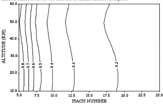
Also of concern in the kinetic studies is the residence time of a fluid element in the combustor. Figure 3.2 plots the inverse of the velocity as a function of Mach number and altitude. The result is a plot of the time required for a fluid particle to traverse one meter, assuming constant velocity. For a combustor on the order of 1.0 m in length, the residence times range from about 0.8 ms at Mach 5 to less than 0.2 ms at Mach 25.

Figure 3.3 shows the pressure and temperature of the fluid delivered to the beginning of the combustor for the second design point. Although the temperatures at high Mach numbers are less than 2400 K, the temperatures at the low end of the trajectory now drop

v iz N4 %--.0 MACH NUMBER

Figure 3.1: Pressure and temperature delivered to the combustor for the first design point. The dotted lines are isotherms marked in Kelvin. The solid lines are isobars marked in atmosphere.

sA n 111 fs

z

Figure 3.2: Residence time per meter of a fluid element in the combustor assuming design point). The times marked are in milliseconds

20.0 22.5 25.0

.--z 60 50 40. 30 20 10 5.0 7.5 10.0 12.5 15.0 17.5 20.0 22.5 25.0 MACH NUMBER

Figure 3.3: Pressure and temperature of the flow delivered to the combustor for the second design point. The dotted lines are isotherms marked in Kelvin. The solid lines are isobars marked in atmosphere.

E

.11 zl

5.0 7.5 10.0 12.5 15.0 17.5

MACH NUMBER

Figure 3.4: Residence time per meter in the combustor for the second design constant residence time, marked in milliseconds.

20.0 22.5 25.0

point. The lines are lines of

to under 600 K. Also, because of the smaller ramp angle, the vehicle must fly a lower trajectory to maintain pressure in the combustor. Pressure at the combustor entrance is 0.5 atm for flight at Mach 5 at about 30 km and Mach 25 at 50 km. The pressure doesn't exceed 5.0 atm for flight above 10 km at Mach 6 or above 18 km at Mach 25. Figure 3.4 shows the residence time per meter of combustor. The residence times per meter are seen to range from slightly above 0.7 ms at Mach 5 to less than 0.2 ms at Mach 25.

Chapter 4

Static Reaction Results

A simple model that provides insight into the underlying nature of the combustion process in the SCRAMJET engine is to consider the SCRAMJET as the combustion chamber in a simple Brayton cycle. The combustion process must, then, by definition, occur at constant pressure. If the details of the injection process are ignored, the momentum equation assures that the velocity is also constant. In this model, the reactions occurring in the SCRAMJET are the same as would occur in a static, constant pressure reaction. The static, constant pressure model is in fact quite useful for investigating the ignition limits and reaction times of a combusting gas. The following sections discuss static, constant pressure reactions for three gas mixtures. The first section examines the H2-air reaction that forms the basis for the SCRAMJET combustion process. As discussed below, however, the combustion limits and reaction times of H2-air combustion make ignition aids necessary over some portions of the trajectory. Two fuel additives are discussed: hydrogen peroxide and silane.

4.0.1 Hydrogen-Air System

The first case considered is hydrogen (H2) combustion in air, where air at standard sea level conditions is

* 78% Diatomic Nitrogen * 21% Diatomic Oxygen * 1% Argon

The reaction mechanism is based on that of Rogers and Schexnayder [11] and consists

of 12 species (H2,°2 ,N2,H ,O ,N ,Ar ,H20 ,OH ,H02 ,H202, and NO) and 23 reaction

paths. Table A.3 (see Appendix A) contains the reactions and the values of the constants for the Arrenhius rate expression in the form of Equation (2.14). Also in Appendix A are the curve fits used for enthalpy calculations.

Using the data shown in the appendix, the kinetic equations of Table 2.2 can be integrated forward in time. Figures 4.1 and 4.2 represent a typical reaction history. The reaction has two distinct phases. The first section of the reaction (0 <T<.25 mS) is the exponential growth of the free radicals caused by the bimolecular dissociation of H2 and 02 (Figure 4.1). During this section of the reaction, the temperature also undergoes an exponential increase (Figure 4.2). In the second part of the reaction, the species begin relaxing to their equilibrium values through a series of relatively slow third body reactions. The temperature still increases substantially in this part of the reaction since much of the reaction's energy is released during the recombination of free radicals.

Two methods for discussing the characteristic time of the reaction are in popular use. The ignition time is defined as the time from the beginning of the reaction to the peak value of OH, and the total reaction time is the time to reach 95% of the equilibrium temperature rise. Since the main concern in the combustor is the total heat release, the second definition will be used.

Figure 4.3 presents the total reaction time of the H2-air system as a function of initial temperature and pressure for an equivalence ratio (the ratio of actual fuel to that required for stoichiometric reaction) of unity. The reaction times were calculated for an initial temperature range of 900 K-1400 K and a pressure range of 0.1-2.0 atm. These values are representative of the conditions expected inside a SCRAMJET combustor.

As clearly indicated in the figure, a strong nonlinearity in the 900 K and 1000 K curves occur at pressures of 0.3 and 1.0 atm respectively. This nonlinearity occurs as the H2-air reaction nears its ignition limit.

The mechanism of the ignition limit can be understood by again referring to Figure 4.1. The rapid breakdown of H2 and 02 into free radicals is led by the creation of hydrogen peroxyl, HO2. The major path of HO2 formation is the third body reaction

M + H + 02 = HO2 + M . Essentially, this chain breaking reaction depletes the supply of atomic hydrogen. Since the reaction is a third body reaction, the rate of reaction (and of atomic hydrogen depletion) increases with increased pressure. Since the formation of free radicals is vital in the initiation of the exponential portion of the reaction, the depletion of atomic hydrogen slows the entire reaction. If the rate of scavenging of H atoms exceeds the rate of H atom production, the reaction stops.

In order to provide regenerative cooling capabilities for the vehicles surface, the vehi-cle's SCRAMJET may actually be operated at an equivalence ratio in excess of 1.0. The reaction times for equivalence ratios greater than 1.0 are investigated in Figure 4.4. In general, increasing the equivalence ratio slightly increases the total reaction times. The

O

0

P

zr

TIME (mS)

Figure 4.1: Time history of the mass fractions in a stoichiometric hydrogen-air reaction with an initial temperature of 1000 K and an initial pressure of 1 atm.

0.95 A T

I

TIME (mS)

Figure 4.2: Time history of the temperature in a stoichiometric hydrogen-air reaction with an initial tem-perature of 1000 K and an initial pressure of 1 atm.

0

0

0

0

o

-1.5 10 -2.0 10 -2.5 10 .- -3.0 V 10 I~r- 5 : lo .4.0 10 -4.5 in 900 K -1 -0.8 -0.6 -0.4 -0.2 o.2 0.4 0.6 10 10 10 10 10 1 10 10 10 PRESSURE (ATM)

Figure 4.3: Total reaction times for the H2-Air system as a function of initial temperature and pressure.

The 900 K and 1000 K lines reach the ignition limit at 0.3 atm and 1.0 atm respectively.

effect is somewhat more noticeable above an equivalence ratio of about 2.5. The two dotted lines in the figure denote pressures above the minimum in the 900 K and 1000 K curves at an equivalence ratio of 1.0. These curves experience greater increased reaction times.

By combining the data of Figures (3.1), (3.2), and (4.3), the required combustor length for complete combustion can be found as a function of altitude and flight Mach number. Figures 4.5 and 4.6 show the required length of constant pressure combustor necessary for complete combustion at the first and second design points, respectively. The combustor lengths are plotted for pressures delivered to the combustor of between 0.1 and 2.0 atm. The low pressure limit is considered to be the limit of effective combustion. The high pressure limit is assumed to provide the lowest practical trajectory that satisfies other aerodynamic constraints on the vehicle. This lower trajectory limit is actually 10 to 20 km lower than the trajectories usually associated with hypersonic vehicles [16]. The lines in the figure are lines of constant combustor length, measured in meters. As clearly seen in

10 -2.0 10 10-2.5

D

Figure 4.4: Effect of equivalence ratio on the H2-Air reaction. The dotted lines denote curves for which

the pressure is above that for minimum reaction time at an equivalence ratio of 1.0

the figures, the required combustor lengths become impractically long as the temperature nears the ignition limit of H₂. For the first design point, the ignition limit is reached for flight below approximately Mach 7.5. For the second design point, the ignition limit is reached below approximately Mach 12.5. Flight below these Mach numbers will required some type ignition aid to initiate combustion. The sections below discuss hydrogen peroxide and silane as possible ignition aids.

The necessity of maintaining sufficient pressure in the combustor can also be seen in Figures 4.5 and 4.6. At low pressures, the third body reactions are less effective, requiring longer combustor lengths to obtain full heat release. A comparison of Figures 4.5 and 4.6 with Figures 3.1 and 3.2 shows that the pressure delivered to the combustor must be greater than about 0.5 atm to maintain combustor lengths less the 3.0 m.

0.1 ATZ4

50.0

40.0

30.0 AT/M

Figure 4.5: Required lengths of the combustor at the fifr- ^

The lines shown e in of the c..

W n inrelff v n Or b s o t t e f r ,.. GV.U OCcur. I-l 1E 111 20

"

U1YIL~~~e-'-

""".L

1

ly

-- --

'A.LiII

E.L)

U'

~

Figure 4.6: Required lengths of the combustor at he seond

design point for complete muson to occur The lines shown are lines of constant length n meters. e desg

1 7.5 10.0 1;wr I, MAnT4 'K' rrr --ZZ.5 2S.0 p4A(-u - rv~LV. ZZ.5,e ,,

4.0.2 Hydrogen-Air-Hydrogen Peroxide System

As discussed above, an ignition aid will most likely be necessary over some portion of the trajectory. Hydrogen peroxide presents an easily available, inexpensive possibility of an ignition aid. The direct attack on the hydrogen peroxide molecule by both free radicals and diatomic molecules, as well as the third body decomposition, cause an abundant supply of free radicals to be produced in the initial stage of the hydrogen-air-hydrogen peroxide reaction. If the free radicals are produced by the decomposition of hydrogen peroxide faster than the scavenging by hydrogen peroxyl, the ignition limit will be overcome.

Figure 4.7 plots total reaction time versus initial temperature and pressure for a mixture of stoichiometric hydrogen/air and 2.5 % mass fraction hydrogen peroxide. The nonlin-earity of the ignition limit is distinctly weakened in the 900 K and 1000 K lines. This is caused by the precise reason given above: the additional formation of free radicals by the decomposition of the hydrogen peroxide. The reaction times for initial temperatures greater than 1200 K are also slightly reduced.

The effect of increasing the mass fraction of H202 at other temperatures and pressures is investigated in Figure 4.8. At temperatures and pressures not affected by the ignition limit (solid lines), increasing amounts of H202 cause slight decreases in the total reaction times. For those temperatures and pressures that are effected by the ignition limit (dotted lines), however, the effect of hydrogen peroxide is to drastically reduce the total reaction times as the ignition limit is overcome.

The data presented so far has been for initial temperatures greater than 900 K. Unfor-tunately, hydrogen peroxide fails to provide an advantage at lower temperatures. Figure 4.9 shows the reaction time as a function of initial temperatures of 750-1000 K and mass fractions of 5% and 10% H202 . Below 900 K, the reaction rates for the decomposition of H20 2 are severely reduced. The reduction in the rate of decomposition of H202 increases the total reaction time. To maintain total reaction times on the order of 1.0 ms, the initial temperature must be greater than about 850 K.

4.0.3 Hydrogen-Air-Silane System

Another possibility for an ignition aid is silane, SiH4. Silane was used in the early ground testing of the Langley Hypersonic Research Engine to facilitate ignition in the subscale test engine.

Unlike H202, silane induces the hydrogen reaction to proceed through a thermal effect. Silane is highly reactive with air at room temperature. When mixed with a H2-air system,

-i -0.8 -0.6 -0.4 -0.2 0.2 10 0.4

10 10 10 10 10 1 10 10 100.6

PRESSURE (ATM) Figure 4.7: Total reaction times

and pressure

for the H2-air-2.5% H202 system as a function of initial temperature

T=900 K, P=.1 ATM T=1000 K, P=.1 ATM T=1200 K, P=.1 ATM ~\ .-. - T=900 K, P=.5 ATM >--- -. =T=900 K, P=1.0 ATM T=1000 K, P=.5 ATM - -,- -T=1200 K, P=.5 ATM

-

Figure 4.8: The effect of increased mass fraction of H202 on the total reaction time for various initial

temperatures and pressure

10 I1C -zrz o 10 10 In I.U -2.0 10 10-2.5 10 10 O v N: -3.0 -3.5 4.0 -4.5 10 10 10 - -

--

----e

\\

---

e

I-

--

=5%

H-0

I

)

Figure 4.9: Effect of hydrogen peroxide as a function of temperature for T< 1050 K

the silane will ignite. If the temperature rise associated with the silane combustion is sufficient, the hydrogen will begin combustion.

The reaction mechanism was assembled from the data for References [17] and [18]. Table A.5 (see Appendix A) contains the reaction mechanism and Arrenhius rate constants. These reactions are in addition to the basic H2-air system of Table A.3.

Figure 4.10 plots the total reaction time versus initial temperature and pressure for a mixture of stoichiometric hydrogen and air plus 2.5% mass fraction silane. As seen in the figure, the nonlinearity in the 900 K and 1000 K lines are almost completely erased. The ignition limit has been overcome by raising the temperature through the initial combustion of silane.

Figure 4.11 shows the effect of varying the mass fraction of SiH4. Similar to the hydrogen peroxide case, the mixtures initially affected by the ignition limit (dotted lines in the figure) experiences drastic decreases in total reaction times. Most of the decrease in reaction times occurs for silane addition accounting for mass fractions less than 2.5%.

4.5--1 10 .8 -. 6 10 .4 -0.2 0 .2 10 0.4 10. PR10 SS10

10 10 1 10 10 10(ATM)

PRESSURE (ATM) Figure 4.10: Total reaction times

temperature and pressure. 10 10 ril U 1-1 w Iz P 10 -2.0 -2.5 -3.0 -3.5 4.0 10-4.5 10 10 10

for the H2-Air-2.5% mass fraction SiH 4 system as a function of initial

T= 900 K, T=1000 K, T=1200 K, Sk I \ \I

_\

MASS FRACTION SiH4

Figure 4.11: Effect of increasing SiH4 on the reaction time. Drastic reductions in reaction time occur for

points above the ignition limit of H2 (dotted lines). More moderate reductions occur at other temperatures

and pressures. 10 1C -2.0 -2.5 -3.0 -3.5 I-V

1-0