HAL Id: hal-00873218
https://hal.archives-ouvertes.fr/hal-00873218
Submitted on 15 Oct 2013
HAL is a multi-disciplinary open access
archive for the deposit and dissemination of
sci-entific research documents, whether they are
pub-lished or not. The documents may come from
teaching and research institutions in France or
abroad, or from public or private research centers.
L’archive ouverte pluridisciplinaire HAL, est
destinée au dépôt et à la diffusion de documents
scientifiques de niveau recherche, publiés ou non,
émanant des établissements d’enseignement et de
recherche français ou étrangers, des laboratoires
publics ou privés.
Guaranteed manipulator precision via interval analysis
of inverse kinematics.
Muhammed R. Pac, Micky Rakotondrabe, Sofiane Khadraoui, Dan O. Popa,
Philippe Lutz
To cite this version:
Muhammed R. Pac, Micky Rakotondrabe, Sofiane Khadraoui, Dan O. Popa, Philippe Lutz.
Guaran-teed manipulator precision via interval analysis of inverse kinematics.. ASME IDETC’13 : ASME 2013
International design Engineering Technical Conference (IDETC) and Computers and Information in
Engineering Conference (CIE), Jan 2013, United States. pp.1-8. �hal-00873218�
Proceedings of the ASME 2013 International Design Engineering Technical Conferences & Computers and Information in Engineering Conference IDETC/CIE 2013 August 4-7, 2013, Portland, Oregon, USA
DETC2013-13033
GUARANTEED MANIPULATOR PRECISION VIA INTERVAL ANALYSIS OF INVERSE
KINEMATICS
Muhammed R. Pac Next Generation Systems Group Department of Electrical Engineering
University of Texas at Arlington Texas 76010
Micky Rakotondrabe AS2M Department FEMTO-ST Institute
University of Franche-Comt ´e (UFC) 25000 Besanc¸on, France
Sofiane Khadraoui Texas A&M University at Qatar Education City, PO Box 23874
Doha, Qatar
Dan O. Popa∗
Next Generation Systems Group Department of Electrical Engineering
University of Texas at Arlington Texas 76010
Email: [email protected]
Philippe Lutz AS2M Department FEMTO-ST Institute
University of Franche-Comt ´e (UFC) 25000 Besanc¸on, France
ABSTRACT
The paper presents a new methodology for solving the in-verse problem of manipulator precision design. Such design problems are often encountered when the end-effector uncer-tainty bounds are given, but it is not clear how to allocate preci-sion bounds on individual robot axes. The approach presented in this paper uses interval analysis as a tool for uncertainty mod-elling and computational analysis. In prior work, the exponential formulation of the forward kinematics map was extended to inter-vals. Here, we use this result as an inclusion function in the com-putation of solutions to set-valued inverse kinematic problems. Simulation results are presented in two case studies to illustrate how we can go from an uncertainty interval at the end-effector to a design domain of allowable uncertainties at individual joints and links. The proposed method can be used to determine the level of precision needed in the design of a manipulator such that a predefined end-effector precision can be guaranteed. Also, the approach is general as such it can be easily extended to any degree-of-freedom and kinematic configuration.
∗
INTRODUCTION
The success of automated assembly by robotic manipulators is highly dependent on the precision of the positioning mecha-nisms employed in the kinematic design of the robot. The im-portance of precision becomes more prominent when the desired operational accuracy is in micro/nano scale as in micro-assembly and nano-manipulation applications. Most of the parametric un-certainties that are negligible in conventional robotics become the predominant error sources in micro/nano applications. With the emergence of micro/nano-robotics in the last decade, there is a growing demand for design guidelines describing how to build these robots based on application specific precision criteria. Since the current methodology have not addressed this problem well, we propose a new approach to the kinematic analysis and design of robots using interval analysis.
In late 80’s and early 90’s, modelling of errors in robot kine-matics was a popular topic [1–6]. However, these works are lim-ited to analysing the effects of general error transformations and do not address how they come about or how to choose or design the parameters of a manipulator for a given end-effector
preci-sion. On the other hand, mechanical design of multi-axis ma-chines based on the accuracy required at the tool tip has been investigated for precision machine design. A concept called er-ror budget was proposed to account for the effect of each erer-ror source on the tool accuracy [7, p. 61], [8]. Using first order and small angle approximations to simplify the homogeneous trans-formation matrices describing geometric errors in the mechanism of a machine, an overall kinematics map can be created to anal-yse the effects of error terms on the tool accuracy. The results of this analysis provide the designer with insight into how to allo-cate mechanical tolerances to the individual system components. However, there is no systematic way of doing this allocation due to the fact that this type of an inverse problem is difficult to pose and solve.
A recent work in [9] studies modular robotic chains made up of individual axes with link/joint uncertainties for several different configurations. It was shown that some of the kine-matic configurations provide more successful operation. Also, joint position uncertainties were shown to manifest themselves as end-effector inaccuracy in different magnitudes depending on the kinematic design. The analysis of error propagation in this work was done using Monte Carlo simulations which suffer from in-ability to provide guaranteed closed form solutions since Monte Carlo method can only solve for sample points and produce sets of points in the solution space.
Finding guaranteed solutions to a set of equations with un-certain data is possible with interval analysis. Interval analysis is a mathematical tool for computation of rigorous bounds on solu-tions to ideal model equasolu-tions when the input arguments of the model are represented as intervals instead of point values. It ex-tends the model equations to the interval domain and allows for analytical and computational handling of uncertain data without having to assume a distribution for it or to sample it. It also helps avoid the complex mathematical formulations involving distribu-tion funcdistribu-tions [10].
Intervals were used in [11] to model uncertain physical pa-rameters of a robot and to find its forward kinematics map using Denavit-Hartenberg (D-H) notation. Optimization of the D-H parameters was done to minimize volumetric end-effector error while optimizing the cost of precision. While this work nicely approaches the problem from a mechanism design perspective, it fails to consider the fact that a mechanism design cannot be op-timized practically without considering the uncertainty in joint positions. Interval analysis was also used in [12] to find the multiple solutions to the forward kinematics problem of paral-lel robots. Then, [13] extends the method to finding the robot parameters that guarantee a singularity-free workspace.
In our prior work [14], the exponential formulation of the forward kinematics map for serial manipulators was extended to intervals. This makes it possible to use interval analysis to find guaranteed precision bounds on the end-effector pose given the uncertainty of the kinematic parameters. The contribution
of the current paper is that we now propose a new method that can solve the inverse problem of bounding the allowable uncer-tainty in kinematic parameters of a manipulator based on given end-effector precision specifications. Besides precision machine designers, this method bears an importance for those roboticists who have to design a manipulator using elementary building blocks. For instance, custom design of multi-axis precision ma-nipulators using individual single-axis stages is a common prac-tice in the micro-assembly area [15–17]. The cost of such stages increase significantly with the increase in motion precision. For a given application, therefore, determining the level of precision required in each axis is an important yet insufficiently addressed consideration.
Next section provides an overview of [14], the forward kine-matics problem with uncertain parameters. Then, we discuss how the precision manipulator design problem can be posed via interval analysis of inverse kinematics. We present simulation results illustrating the use of our method for a simple 2-link ma-nipulator and a 3-DOF PPR stage, a commonly used robot in pre-cision assembly. Finally, the paper is concluded with references at the end.
FORWARD KINEMATICS WITH UNCERTAIN JOINT PA-RAMETERS
Kinematic description of a robot involves certain parame-ters such as link lengths and joint axis vectors. In an ideal robot model, these are all assumed to be perfectly precise values. A practical implementation, however, requires calibrating the robot to minimize the uncertainty in the knowledge of such constants. Even with calibration, identification of kinematic parameters can only be done with a limited precision. Robot kinematics also in-volves joint position variables which are known to a limited pre-cision as well. Therefore, there needs to be a kinematic model that can handle these uncertainties with ease and efficiency.
Using the screw-based exponential formulation [18] and in-terval analysis [10], we formulated the inin-terval extension of for-ward kinematics map in [14]. The advantage of the exponential formulation over D-H parameters is that the joint parameters can be described with respect to the world reference frame which is the frame of reference used in the description of precision met-rics. We model uncertain parameters and variables of a robot with intervals. For example, a (real) interval such as x [1,2] is a closed set of real numbers represented by the two boundary values, 1 is called the left endpoint and 2 is called the right end-point. In this paper, we follow the notation in [19] and denote intervals with square bracketed letters.
For a revolute joint, the interval extension of the homoge-neous transformation matrix, [T], can be represented with the function in (1) where[ω]is the joint axis vector, [ ˆω]is the skew-symmetric matrix of[ω], [θ] is the joint displacement, and [q] is a point along the joint axis. Note that in exponential formula-2 Copyright © 2013 by ASME
tion, joint transformations are with respect to the base reference frame.
[T]([ω],[θ],[q]) e[ ˆω][θ]0 (I −e[ ˆω][θ]1 )[q] (1) In equation (1),[T]([ω],[θ],[q]) is called an inclusion func-tion since it covers all possible homogeneous transformafunc-tion ma-trices T(ω,θ,q) of the special Euclidean group SE(3) that can be obtained by varying the arguments ω, θ , and q in the respective ranges of[ω], [θ], and [q].
Similarly for a prismatic joint, the interval extension for the joint transformation is represented with the inclusion function in (2) where[d] is the joint displacement and [v] is the joint axis vector. The rotation part of the transformation denoted with[R]is ideally a 3×3 identity matrix. In an actual linear axis, however, tilt error of the stage may also play an important role. Hence, this part can be modelled as a general rotation transformation [R]= e[ ˆω][θ].
[T]([d],[v]) [R] [d][v]0 1 (2) Finally, interval extension of the forward kinematics map of a serial manipulator with n joints can be written as
[f]([x]) = [T1]···[Tn]·[f]([x0]) (3)
where[f] represents the inclusion function for the forward kine-matics map and[x]is the vector of joint parameters and variables. For further details on the forward kinematics map, the reader is referred to [14].
INTERVAL ANALYSIS OF INVERSE KINEMATICS Computing the joint angles of a manipulator for a given end-effector pose is called inverse kinematics. There are two main types of solution to this problem: closed-form solutions and numerical solutions [20, p. 106]. Closed-form solutions are based on analytical expressions of the inverse relationship be-tween joint angles and end-effector pose. Due to the complex nonlinear nature of robot kinematic equations, finding a closed-form solution is difficult in general. On the other hand, numerical solutions rely on the description of forward kinematics map and repeated evaluation of approximate joint angles until the desired end-effector configuration is sufficiently approached.
Inverse Kinematics with Joint Parameter Uncertainty: An Example
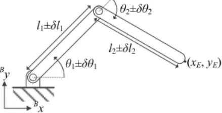
Consider the simple example shown in Fig. 1 where a two-link planar manipulator with revolute joints is depicted. The
l1±δl1 θ1±δθ1 θ2±δθ2 l2±δl2 Bx By (xE, yE)
FIGURE 1: TWO-LINK MANIPULATOR WITH UNCERTAIN
LINK LENGTHS AND JOINT ANGLES.
knowledge of the link lengths and joint positions are assumed to be uncertain to the extent denoted by δ liand δ θifor i= 1,2,
respectively. Given the nominal link lengths liand joint positions
θi, the corresponding interval arguments can be expressed as
[x] [l1] [θ1] [l2] [θ2] [l1−δl1,l1+δl1] [θ1−δθ1,θ1+δθ1] [l2−δl2,l2+δl2] [θ2−δθ2,θ2+δθ2] . (4)
It was shown in [14] that the rotation part of the revolute joint transformation in (1) reduces to the interval extension of the Rodrigues’ formula when the joint axis is a real (point-valued) vector as in the case of this example. That is,
R(ω,[θ]) eωˆ[θ]= I + ˆω sin([θ])+ ˆω2(1−cos([θ])) (5) where ω = (0,0,1)Tis a real vector for the manipulator in Fig. 1. Then, the inclusion function for the transformation of the end effector pose can be written as
[f]([x]) = [T](ω1,[θ1],[q1])·[T](ω2,[θ2],[q2])·[f]([x0]) (6)
where
[T](ωi,[θi],[qi]) = R(ωi,[θi]) (I −R(ωi,[θi]))[qi]
0 1 . (7)
Then, the inverse problem for this mapping can be posed as fol-lows:
For a given interval of end-effector position [y]= [f]([x]), what should be the manipulator parameters [x]= ([l1],[θ1],[l2],[θ2])T?
Note that the answer to the above question can provide not only the range of[θi]for the desired interval of end-effector
posi-tion but also the maximum allowable uncertainty in[θi] and [li].
design of manipulators. That is, determination of the required joint encoder resolution and of the manufacturing tolerance for the robot mechanism can be done based on the results of this inverse kinematic analysis.
When the kinematic mechanism is as simple as the one in Fig. 1, the point-valued inverse kinematics problem can be solved analytically as in (8) [20, p. 112]. These equations pro-vide a couple of solutions for θ1and θ2for each end-effector
po-sition(x,y). However, as the number of joints increases, the for-ward kinematics map becomes non-invertible. Also, incorpora-tion of mechanism errors and parameter uncertainties introduces additional degrees of freedom to the formulation. Then, finding the inverse solution with interval arguments requires a set-based computational method. In order to address this problem, next we will introduce a set inversion algorithm that is based on interval analysis. θ2= ±cos−1(x 2+y2−l2 1−l22 2l1l2 ) θ1= atan2(y,x) cos−1(x2+y2+l21−l22 2l1 √ x2+y2 ) (8)
Set Inversion via Interval Analysis
Given a nonlinear function f fromRntoRmand a setY in Rm, findingX described as
X = {x ∈Rn| f(x) ∈Y}= f−1(Y)
(9)
is the set inversion problem [19, p. 55]. Jaulin et al. addressed this problem via an algorithm called SIVIA (Set Inversion Via Interval Analysis) [21]. For a givenY ∈Rm,X can be bounded
arbitrarily closely with a lower boundX and an upper bound X such thatX ⊂ X ⊂ X provided that an inclusion function [f] can be found for f. Note that X is guaranteed to be a solution set whereasX may contain non-solution points.
The process of findingX using SIVIA is illustrated in Fig. 2 for 2-dimensional x and y spaces. SIVIA starts with an initial search domain [x0] that is guaranteed to contain X. Then, the
following 4-step procedure is applied:
If the mapping[f]([x]) results in an interval (box) in the y-space that intersects withY without being fully enclosed by Y as in Fig. 2(a), then [x] is said to contain part of the so-lution setX but regarded as undetermined. If the width of [x] is greater than a predetermined resolution parameter ε, then it needs to be bisected along the longest side and the procedure needs to be repeated recursively on each sub-box. If[f]([x]) ∩Y = /0 as in Fig. 2(b), then [x] is not part of X hence can be discarded.
If[f]([x]) ⊂ Y as in Fig. 2(c), then [x]⊂ X and [x]∈X and [x]∈X. x1 x2 [x0] y1 y2 X [f] Y x1 x2 [x1] X [f] y1 y2 Y (a) (b) x1 x2 [xn] X [f] y1 y2 Y (d) x1 x2 [xn] X [f] y1 y2 Y (c)
FIGURE 2: SIVIA ALGORITHM PROCEDURE (BASED ON
[19, p. 57]).
Finally, if[x] is undetermined and width([x]) < ε as in Fig. 2(d), then the procedure stops for[x] and it is added to the upper boundX of X.
General Case of Inverse Kinematics via Set Inversion Let f be the forward kinematics map of a serial manipulator fromRnto SE(3) where n is the total number of joint variables and parameters that are uncertain. Also, let Y be a subset of SE(3). Then, calculatingX in (9) is the inverse kinematics prob-lem in presence of joint parameter uncertainties for a given set of end-effector configurations. This is inherently a set inversion problem and can be addressed using SIVIA.
Application of SIVIA to a general inverse kinematics prob-lem requires comparing [f]([x]) in (3) with Y and determining whether or not they intersect or one includes the other. This is relatively simpler if Y can be represented as an interval so that both[f]([x]) and Y are 4×4 interval matrices. Then, the compar-ison can be done element-wise. Otherwise, each member ofY has to be compared with[f]([x]) one by one.
SIMULATIONS
In this section, we present some example simulation results that show how the proposed method can be implemented. We carried out interval calculations using MATLAB and a toolbox called INTLAB developed by S. M. Rump [22]. INTLAB sup-ports many operations with real and complex interval scalars, vectors, and matrices. It provides efficient functions for basic operations in algebra, trigonometry, etc.
In order to verify the results obtained using interval analy-sis, we also performed Monte Carlo analysis. When an analytical expression for inverse kinematics is available, it can directly be used to go from the configuration space to the parameter space. For instance, by evaluating equation (8) for various samples of 4 Copyright © 2013 by ASME
TABLE 1: TWO-LINK MANIPULATOR SIMULATION PA-RAMETERS.
l1 δ l1 l2 δ l2 [θ1(0)] [θ2(0)]
1 0.001 1 0.001 [0,π/2] [−π/2,π/2]
the input arguments[l1], [l2], [x], and [y], one can obtain a set of
points in the joint space whose convex hull approximately pro-vides the inverse solutionX. We refer to this as the Monte Carlo solution in the next part.
Precision Design of the Two-Link Manipulator
In this part, we present the solution to the inverse kinematics problem of the two-link manipulator discussed in . This serves as a validation example such that we verify the interval analysis results with Monte Carlo simulation of inverse kinematic equa-tions. The results will enable us to determine the minimum joint encoder resolution required to achieve a given end-effector pre-cision.
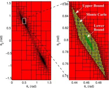
For the manipulator parameters given in Table 1 and for a sample end-effector position([x],[y]) = (1.4±0.01,1.2±0.01), the solutions of the SIVIA algorithm for a stopping criterion of ε=π/1800is shown in Fig. 3. The picture on the left shows the
7018 subpavings (i.e. bisected arguments) of θ1and θ2each of
which represent an interval sample from the joint space. SIVIA produces increasing concentration around the two solution re-gions as it converges by bisecting initial ‘undetermined’intervals. The exploded view of one of those regions on the right shows that the remaining undetermined regionX (yellow) found by SIVIA properly encloses the inverse Monte Carlo solutionX (blue line) which in turn encloses the lower boundX (green region) as sug-gested by SIVIA.
The result in Fig. 3 shows that if the joint positions can be addressed as precisely as to fit in the lower bound (green region, X), then it can be guaranteed that the end-effector can be posi-tioned in the given interval ([x],[y]) = (1.4 ±0.01,1.2 ±0.01). The question is then how to quantify the precision based on this result.
Fig. 4(a) shows X in more detail where an interval of (θ1,θ2) with the largest overlapping area with X is encircled.
If the length of this interval along θ1 is A and that along θ2
is B, then the proper design choice for the joint resolution of the manipulator about these two axes can be described as in equation (10). This makes sure that the actual joint positions [θ1] [θ1−δθ1,θ1+δθ1] and [θ2] [θ2−δθ2,θ2+δθ2] can
be commanded to be insideX for a certain value of θ1and θ2.
This is explained pictorially in Fig. 4(b) with an arbitrarily posi-tioned grid of addressable intervals each of which represents the
0 0.5 1 1.5 −1.5 −1 −0.5 0 0.5 1 1.5 θ 1(rad) θ2 (rad) 0.44 0.46 0.48 0.74 0.76 0.78 0.8 0.82 0.84 0.86 θ 1(rad) θ2 (rad) Monte Carlo Upper Bound Lower Bound
FIGURE 3: BOUNDS ON θ1 AND θ2 OF THE TWO-LINK
MANIPULATOR FOR([x],[y]) = (1.4±0.01,1.2±0.01). set of actual joint positions for a given position command. When the condition in (10) is satisfied, there exists at least one interval of([θ1],[θ2]) that completely overlaps with X. In Fig. 4(b), there
are five such possible joint positions shown by boxes with the slash pattern. Therefore, δ θ1∗and δ θ2∗are the coarsest resolution values for the joint encoders that guarantee the given end-effector precision. In this case, (A,B) is measured to be (π/900,π/450)
which correspond to (δθ1∗,δθ2∗) = (0.05°,0.1°). For this par-ticular end-effector position, it can be seen that the resolution requirement for the first joint is higher as it can introduce more Abbe error due to its distance from the end-effector.
δ θ1≤ δθ∗
1 A/4 , δ θ2≤ δθ2∗ B/4 (10)
The lower boundX can always be improved in expense of computational time by reducing the value of ε. Fig. 5(a) com-pares the previous result in Fig. (3) where ε was π/1800 with
the one in Fig. 5(b) where ε is π/3600. It can be seen that a
finer bisection resolution improves the lower boundX towards the Monte Carlo result. The amount of improvement in this case is from (A,B) = (π/900,π/450) to (A,B) = (7π/3600,π/400) which
means that the δ θ1∗and δ θ2∗are now 0.0875° and 0.1125°, re-spectively. The total number of subpavings processed in this case is 57590 which is significantly higher than the previous value 7018. Indeed, SIVIA terminates after generating less than (width([x0])/ε+1)nbisections while the computing time increases
propor-0.46 0.465 0.47 0.78 0.785 0.79 0.795 0.8 0.805 0.81 θ 1(rad) θ2 (rad) B A (a) 0.46 0.465 0.47 0.78 0.785 0.79 0.795 0.8 0.805 0.81 1(rad) 2 (r a d ) B/2 A/2 (b)
FIGURE 4: (a) THE INTERVAL OVERLAPPING WITH THE
LOWER BOUND X WITH MAXIMUM AREA OF A × B (b) AN ARBITRARILY POSITIONED GRID OF ADDRESS-ABLE INTERVALS FOR δ θ1=A/4AND δ θ2=B/4.
tional to the number of degrees of freedom of a manipulator. However, using bisections is one of the most basic techniques of interval analysis in terms of computational efficiency. There are efficient solvers that combine use of bisections, contractors, inclusion tests, and local optimization procedures to reduce the computational complexity to polynomial order [19]. Application of these solvers to the inverse kinematics problem is not covered in this paper but will be addressed in the future.
Allocation of Mechanism Tolerances in a 3-DOF Preci-sion Stage
In this part, we will demonstrate how the presented method can also be used to allocate tolerances to the mechanical design of a 3-DOF PPR manipulator as in Fig. 6 such that a given end-effector precision can be achieved. For clarity, we will focus only on some of the parametric uncertainties of the manipula-tor such as prismatic joint axes and rotary joint position vec-tors. The presented method will enable us to bound the allow-able misalignment in these vectors. The vectors[vx], [vy], and
[q] that parametrize the manipulator are represented as shown in (11) with error bounds denoted by[δvy] for the misalignment of
[vx] along y-axis, [δvx] for the misalignment of [vy] along x-axis,
and[δq] for the misalignment of [q] along x and y axes. In a practical scenario, for instance, these terms can represent the er-rors introduced into the geometry of the manipulator during its manufacturing or assembly. 0.44 0.46 0.48 0.74 0.76 0.78 0.8 0.82 0.84 1(rad) 2 (r a d ) Upper Bound Monte Carlo Result Lower Bound (a) 0.44 0.46 0.48 0.74 0.76 0.78 0.8 0.82 0.84 1(rad) 2 (r a d ) Upper Bound Monte Carlo Result Lower Bound (b)
FIGURE 5: UPPER (X) AND LOWER (X) BOUNDS FOUND
USING SIVIA AND (X) FOUND USING MONTE CARLO FOR (a) ε=π/ 1800(b) ε=π/3600. [vx] [vy] ω x y z [q]
FIGURE 6: 3D MODEL OF A 3-DOF PPR PRECISION
MO-TION STAGE. [vx]= 1 [δvy] 0 [vy]= [δvx] 1 0 [q]= [δq] [δq] 0 (11)
The objective in this simulation is to find how large [δvy],
[δvx], [δqx], and [δqy]can be for a given stage positioning
preci-sion. For example, assume a configuration attached to the rotary stage needs to be driven from an initial pose pito a final pose pf
-200 0 200 -200 -100 0 100 200 -150 -100 -50 0 50 100 150 v y( m) vx( m) q ( m ) δvx δvy δq (a)
-30um -15um 0.207m +15um +30um
-30um -15um 0.407m +15um +30um x-axis (m) y -a x is (m )
Allowed final position
Monte Carlo results
(b)
FIGURE 7: (a) BOUNDING OF ERROR TERMS [δvy],
[δvx], and [δq] (b) END-EFFECTOR POSITION BY MONTE
CARLO SAMPLING OF (13).
through the manipulator transformation that can be described as
[pf]= I dx[vx] 0 1 I dy[vy] 0 1 eωθˆ (I −eωθˆ )[q] 0 1 pi (12)
where dx, dy, andθ are the desired displacements of the axes. We
chose the initial end-effector position to be(10mm,0mm,0°) and final joint position to be(200mm,400mm,45°). Then, we solved for[δvy], [δvx], and [δq]that guarantee a maximum deviation of
30µm from the desired final position. Fig. 7(a) shows the lower bound solution of this simulation. Similar to the previous case, the largest interval box that can be fit into the lower bound has approximate dimensions of (60,140,13) µm. Then from (10), the allowable maximum uncertainty in the axes vectors can be expressed as
[δvx]= [−15,15]µm
[δvy]= [−35,35]µm
[δq]= [−3.25,2.25]µm. (13) Fig. 7(b) shows the distribution of end-effector position by sampling the intervals in (13) using Monte Carlo method. It can be seen that the results all lie inside the allowed boundary for fi-nal end-effector position hence (13) is a guaranteed tolerance al-location. It can also be seen in (13) that the amount of allowable uncertainty is different for different parameters. This depends on the given initial and final positions, desired stage positioning precision, and the kinematic design. Hence, the result can also be used to do sensitivity analysis to find out which parameter is likely to cause more deviation at the end-effector.
CONCLUSIONS
In this paper we propose a methodology for solving manip-ulator design problems with precision bounds. The simulation results show that the proposed method is effective in determining the level of precision needed in the design of a manipulator for a given end-effector precision. Solution of the inverse kinemat-ics problem using interval analysis not only provides the range of joint space variables for a desired end-effector position but also allows calculation of the maximum allowable uncertainty in the joint sensor (encoder) feedback and the mechanism geome-try tolerances. Therefore, the method can be used as a design aid in robotic applications that involve designing, building, or choosing individual axes of a multi-degree-of-freedom manipu-lator. Since we use standard interval analysis tools such as SIVIA algorithm, our approach can easily be applied to any kinematic configuration. Future work will include using heuristics to speed up the computational efficiency of the algorithm and exercising this method on the design of a modular micro-assembly robot.
REFERENCES
[1] Benhabib, B., Fenton, R., and Goldenberg, A., 1987. “Computer-aided joint error analysis of robots”. IEEE Journal of Robotics and Automation, 3(4), Aug., pp. 317– 322.
[2] Lin, P., and Ehmann, K., 1993. “Direct volumetric error evaluation for multi-axis machines”. International Journal of Machine Tools and Manufacture, 33(5), Oct., pp. 675– 693.
[3] Shin, Y., and Wei, Y., 1992. “A statistical analysis of posi-tional errors of a multiaxis machine tool”. Precision Engi-neering, 14(3), July, pp. 139–146.
[4] Soons, J., Theuws, F., and Schellekens, P., 1992. “Model-ing the errors of multi-axis machines: a general methodol-ogy”. Precision Engineering, 14(1), Jan., pp. 5–19. [5] Vaishnav, R. N., and Magrab, E. B., 1987. “A general
pro-cedure to evaluate robot positioning errors”. International Journal of Robotics Research, 6(59), Mar., pp. 59–74. [6] Veitschegger, W., and Wu, C.-H., 1986. “Robot accuracy
analysis based on kinematics”. IEEE Journal of Robotics and Automation, 2(3), Sept., pp. 171–179.
[7] Slocum, A. H., 1992. Precision Machine Design. Society of Manufacturing Engineers, Dearborn, MI, USA.
[8] Frey, D. D., 2004. Robotics and Automation Handbook. CRC Press, ch. 10.
[9] Das, A. N., and Popa, D. O., 2011. “Precision evaluation of modular multiscale robots for peg-in-hole microassembly tasks”. In IEEE/RSJ Int. Conf. on Intelligent Robots and Systems, pp. 1699–1704.
[10] Moore, R. E., Kearfott, R. B., and Cloud, M. J., 2009. In-troduction to Interval Analysis. Society for Industrial and Applied Mathematics, Philadelphia, PA, USA.
[11] Wu, W., and Rao, S. S., 2007. “Uncertainty analysis and allocation of joint tolerances in robot manipulators based on interval analysis”. Reliability Eng. and System Safety, 92, pp. 54–64.
[12] Merlet, J. P., 2004. “Solving the forward kinematics of a goughtype parallel manipulator with interval analysis”. Int. J. of Robotics Research, 23(3), p. 221236.
[13] Merlet, J. P., 2009. “Interval analysis for certified numer-ical solution of problems in robotics”. International Jour-nal of Applied Mathematics and Computer Science, 19(3), pp. 399–412.
[14] Pac, M., and Popa, D., 2012. “Interval analysis for robot precision evaluation”. In Proc. 2012 IEEE Interna-tional Conference on Robotics and Automation (ICRA), pp. 1087–1092.
[15] Dechev, N., Cleghorn, W. L., and Mills, J. K., 2004. “Mi-croassembly of 3-d microstructures using a compliant, pas-sive microgripper”. Journal of Microelectromechanical Systems, 13(2), Apr., pp. 176–189.
[16] Probst, M., C. Hrzeler, R. B., and Nelson, B. J., 2009. “A microassembly system for the flexible assembly of hy-brid robotic mems devices”. International Journal of Op-tomechatronics, 3(2), pp. 69–90.
[17] Das, A. N., Murthy, R., Popa, D. O., and Stephanou, H. E., 2012. “A multiscale assembly and packaging sys-tem for manufacturing of complex micro-nano devices”. IEEE Transactions on Automation Science and Engineer-ing, 9(1), pp. 160–170.
[18] Murray, R. M., Li, Z., and Sastry, S. S., 1994. A Mathemat-ical Introduction to Robotic Manipulation. CRC Press. [19] Jaulin, L., Kieffer, M., Ditrit, O., and Walter, E., 2001.
Ap-plied Interval Analysis. Springer-Verlag, London, Great Britain.
[20] Craig, J. J., 2005. Introduction to Robotics: Mechanics and Control, third ed. Pearson Prentice Hall, NJ, USA. [21] Jaulin, L., and Walter, E., 1993. “Set inversion via interval
analysis for nonlinear bounded-error estimation”. Automat-ica, 29(4), Nov., pp. 1053–1064.
[22] Rump, S. M., 1999. “Intlab interval laboratory”. In Devel-opments in Realiable Computing, T. Csendes, ed. Kluwer Academic Publishers, Dordrecht, pp. 77–104.
[23] Jaulin, L., and Walter, E., 1993. “Guaranteed nonlinear parameter estimation from bounded-error data via inter-val analysis”. Mathematics and Computers in Simulation, 35(2), Apr., pp. 123–137.
![FIGURE 2 : SIVIA ALGORITHM PROCEDURE (BASED ON [19, p. 57]).](https://thumb-eu.123doks.com/thumbv2/123doknet/8012113.268518/5.918.483.857.110.322/figure-sivia-algorithm-procedure-based-on-p.webp)