Explaining the Transition Between Exchange Rate Regimes

Cahier 2003-21

MASSON, Paul

RUGE-MURCIA, Francisco J.

Explaining the Transition Between Exchange Rate

Regimes

Département de sciences économiques

Université de Montréal

Faculté des arts et des sciences C.P. 6128, succursale Centre-Ville Montréal (Québec) H3C 3J7 Canada http://www.sceco.umontreal.ca SCECO-information@UMontreal.CA Téléphone : (514) 343-6539 Télécopieur : (514) 343-7221

Ce cahier a également été publié par le Centre interuniversitaire de recherche en économie quantitative (CIREQ) sous le numéro 15-2003.

This working paper was also published by the Center for Interuniversity Research in Quantitative Economics (CIREQ), under number 15-2003.

Explaining the Transition Between

Exchange Rate Regimes

¤

Paul Masson

Brookings Institution

Francisco J. Ruge-Murcia

University of Montreal

June 2003

This paper studies the transition between exchange rate regimes using a Markov chain model with time-varying transition probabilities. The probabilities are parame-terized as nonlinear functions of variables suggested by the currency crisis and optimal currency area literature. Results using annual data indicate that in°ation, and to a lesser extent, output growth and trade openness help explain the exchange rate regime transition dynamics.

JEL Classi¯cation: F33

Key Words: Exchange rates, hollowing out hypothesis, regime change, Markov chains, pegs, °oating

¤_{The views expressed here are those of the authors and do not commit their respective institutions. We}

are grateful to Susan Collins and Paolo Mauro for comments, and to Grace Juhn, Haiyan Shi, and Saji Thomas for research assistance. The second author thankfully acknowledges the ¯nancial support from the Social Sciences and Humanities Research Council and the Fonds pour la Formation de Chercheurs et l'Aide µa la Recherche. Correspondence: Francisco J. Ruge-Murcia, D¶epartement de sciences ¶economiques, Universit¶e de Montr¶eal, C.P. 6128, succursale Centre-ville, Montr¶eal (Qu¶ebec) H3C 3J7, Canada. E-mail: francisco.ruge-murcia@umontreal.ca

Résumé

Pour étudier la dynamique du passage entre différents régimes de taux de change, cet article utilise un modèle markovien dont les probabilités de transition varient dans le temps. Ces probabilités sont modélisées par des fonctions non linéaires de variables que nous ont suggérées les littératures sur les zones monétaires optimales et sur les crises de change. En nous basant sur des données annuelles, nous trouvons que l'inflation et, dans une moindre mesure, la croissance de la production et l'ouverture au commerce expliqueraient en partie les dynamiques de transition des régimes de taux de change.

Mots clés: taux de change, hollowing out hypothesis, changement de régime, chaîne de Markov, taux de change fixe, taux de change flottant

1

Introduction

Advocates of the \hollowing out" hypothesis argue that the increase in capital mobility would tend to make intermediate exchange rate regimes (for example, adjustable pegs, bands, or dirty °oating) disappear, in favor of the extremes of currency boards or monetary union on the one hand, and freely °exible exchange rates on the other [see Eichengreen (1994), Obstfeld and Rogo® (1995), and Fischer (2001)]. Underlying this view is the presumption that the abandonment of intermediate exchange rate regimes would not be the result of a voluntary choice. Instead, if countries attempted to maintain an intermediate regime until forced to exit, it would be the result of a speculative attack [see Eichengreen et al. (1999)]. The adoption of a regime would be less the result of o±cial policy than of speculators' actions. An exchange rate peg would give way to a °oating currency if the former was unsustainable as a result of over-expansionary domestic credit (as in ¯rst generation models), or low growth and high unemployment (as in second generation models). In principle, the abandonment of an intermediate exchange rate regime in a crisis could also involve a move to a currency board or monetary union, though in practice this is less frequent.

A parallel and equally in°uential literature on exchange rate regime choice is derived from Mundell's seminal paper on optimum currency areas (OCA). The structural characteristics of an economy should in°uence whether a country would choose to share a common currency with another. These characteristics include, for example, the correlation (symmetry) and e®ect of shocks and the mobility of labor [Mundell (1961)]. Other factors have also been suggested as important for the choice of exchange rate regime, such as the existence of ¯scal transfers, the degree of openness, and the extent of diversi¯cation of production [see Masson and Taylor (1993) for a survey]. Though there have been numerous attempts to explain regime choice using OCA models, the variables implied by the theory have not been very successful in accounting for the observed exchange rate regimes [see, for example, Frankel and Rose (1998), Mussa et al. (2000), and Juhn and Mauro (2001)]. Poirson (2001) reports some success of traditional OCA variables and political factors in explaining regime choice. Masson (2001) argues that a strategy to test the hollowing out hypothesis is to look at the matrix of transition probabilities between di®erent exchange rate regimes.1 Speci¯cally, one can test whether there are transitions away from intermediate regimes, but not towards them. This condition is both necessary and su±cient for hollowing out. Using two di®erent exchange rate regime classi¯cations, the data generally reject the hollowing out hypothesis for all time periods when all countries are included. When the sample is restricted to the

1_{Markov chains have been used in other contexts to study the properties of long-run distributions, for}

decade of the 1990s for the emerging market countries only, and for only one of the two regime classi¯cations, the data cannot reject the hypothesis that there are no exits from currency boards, implying that this regime would eventually dominate. Such a conclusion contrasts with the predictions of OCA models, which imply that a degree of exchange rate °exibility would be desirable, hence that countries would prefer an intermediate regime.

This paper estimates a Markov chain model of exchange rate regime transitions with time-varying probabilities. In particular, the transition probabilities between exchange rate regimes are speci¯ed to be nonlinear functions of the explanatory variables. The explanatory variables are those implied by both OCA and currency crisis models. Results indicate that in many cases, it is possible to reject the null hypothesis of constant transition probabilities, in favor of an alternative where in°ation, trade openness, output growth, and/or reserves help determine exchange rate regime transitions. We also study whether, conditioning on unchanged explanatory variables, transitions have changed over time. For instance, if capital mobility has increased, then the currency crisis literature predicts that transitions away from intermediate regimes should increase. Finally, we test whether industrial and developing countries can be considered to be part of the same sample, or whether they form distinct groups. The latter point has been argued by, for example, Hausman et al. (1999) and Calvo and Reinhart (2002), who suggest reasons why developing countries do not bene¯t from exchange rate °exibility.

Markov chains are also a natural framework to test the predictive power of models that seek to explain the observed distribution of exchange rate regimes. According to currency crisis models, abandonment of pegs should be more frequent when countries with pegs ex-perienced excessive domestic credit growth, overvalued exchange rates, or weak economic activity. According to OCA models, exchange rate regime transitions should result from changes in structural characteristics. These two models are not mutually exclusive. For example, if forced to exit from an adjustable peg, a country's authorities may then have the choice between a hard peg and a free °oat, so both currency crisis and optimum currency area criteria could be relevant. Second generation currency crisis models acknowledge that exit could be a deliberate choice of the authorities, even if provoked by speculation. Thus, a model explaining transitions between exchange rate regimes may include variables implied by bothOCA (or other structural) models and currency crisis models.

The rest of the paper is structured as follows. Sections 2 describes models exchange rate regime choice that motivate our empirical analysis. Section 3 explains the use of Markov chains to model exchange rate regime transitions. Section 4 reports empirical results and examines the ability of the estimated Markov chain model to forecast exchange rate regime transitions. Finally, Section 5 concludes and discusses avenues for future research.

2

Models of Voluntary and Involuntary Exchange Rate

Regime Choice

The main di®erence between OCA (and other structural) and currency crisis models is that the former assume that the exchange rate regime choice is the outcome of a voluntary decision by the monetary authorities. The latter explain the involuntary exit from an exchange rate peg as triggered by the actions of speculators. If a forced exit involves a choice between the alternative regimes, then voluntary and involuntary elements would both be present.

Among the models of voluntary choice of regime, those broadly characterized as opti-mum currency area models have attracted the most attention. In principle, these models should use exogenous structural features of the economy to explain the voluntary choices of the policy authorities. Frankel and Rose (1998) question the exogeneity of some of these variables. Subject to this caveat, several OCA variables have unambiguous implications for the choice of exchange rate regime choice. Poirson [Poirson (2001, Table A4)] identi¯es trade openness, the existence of a dominant trading partner, labor mobility, and nominal °exibility as variables associated witha ¯xed exchange rate regime; and economic develop-ment, diversi¯cation of production and exports, and (large) size of the economy as variables associated witha °oating exchange rate regime. Poirson identi¯es two other sets of models, namely those inspired by political economy [especially Collins (1996) and Edwards (1996)] and by \fear of °oating" [Calvo and Reinhart (2002)]. Political economy or \fear of °oating" variables that have been suggested to in°uence regime choice include the extent of foreign currency debt and dollarization, the degree of central bank credibility, and the size of re-serves. However, some of these variables are very hard to measure, while others are clearly endogenous.

First generation currency crisis models describe the process by which foreign exchange reserves are depleted by speculators [see, for example, Krugman (1979)]. Speculators cor-rectly anticipate that the authorities will not be able to maintain the peg. In the simplest monetary model, the peg is unsustainable because domestic credit expansion is too rapid. In more elaborate models, the peg is unsustainable because the real exchange rate is overvalued or the ¯scal de¯cit is too large.

In second generation models, the authorities are assumed to decide whether to maintain a peg in the light of variables that enter their objective function. Assuming that they care about boththe real economy (e.g., the rate of unemployment) and price (or exchange rate) stability, shocks to the real economy may a®ect the trade-o® between them and lead to a greater willingness to sacri¯ce price (or exchange rate) stability and hence abandon an exchange rate peg.

Currency crisis models suggest a set of largely endogenous variables as determinants of the exchange rate regime. These variables include the rate of domestic credit expansion, th e ¯scal de¯cit, th e level of reserves, th e real exch ange rate, th e rate of unemployment, the growth rate of GDP, and the in°ation rate. In addition, these models suggest that the degree of capital account openness should matter for the vulnerability to speculative attack. Most models assume perfect capital mobility, but if the economy is cut o® from world capital markets, it may not be forced to abandon a peg even in the face of a fundamental disequilibrium.

3Markov Chains

A Markov chain is a simple stochastic structure that can summarize the transition between exchange rate regimes. De¯ne bys_tthe exchange rate regime in periodt: In the analysis that follows,s_t is assumed to take either of three possible values: s_t = 1 denotes a ¯xed exchange rate regime, st = 3 denotes a °oating exchange rate, and st = 2 denotes an intermediate exchange rate regime. The Markov chain is de¯ned by three objects. First, the state-space set, S_t; that contains the possible values the state variable can take (in this case, 1; 2; or 3). Second, th e 3£ 3 matrix of transition probabilities, P; withelements p_ij for i; j = 1;2; 3 :

P = 2 6 4 p11 p12 p13 p21 p22 p23 p31 p32 p33 3 7 5: (1)

The typical element p_ij = Pr(s_t =jjs_t¡1 =i) is the probability that the current regime is j given that the regime in the previous period was i: Third, th e 1 £ 3 vector ¼_t that records the proportion of countries in each of the three regimes at time t: The matrix P satis¯es

P

j pij = 1 for j = 1; 2;3: That is, the elements of P add up to one across rows. Th e vector ¼t satis¯es P

i ¼t;i = 1; where ¼t;i is the typical element of ¼t: The distribution of exchange rate regimes evolves over time following the law:

¼t =¼t¡1P: (2)

Iterating forward on (2) delivers the distribution at some point in the inde¯nite future :

¼ = lim_t!1¼0Pt; (3)

where ¼₀ denotes the initial distribution at time t = 0: Provided that the Markov chain is ergodic, meaning that the matrix P has a single unit eigenvalue, the long-run distribution ¼ is independent of the initial distribution and can be termed the invariant distribution.

The hypothesis of hollowing out of intermediate regimes implies that the second element of¼ is 0. That is, the long-run distribution of exchange rate regimes is concentrated in either one or both of the tails. This is only possible, if either the ¯x, °oating, or both regimes are absorbing states (i.e., p₁₁ = 1 and/or p₃₃= 1) so that other states cannot be reached from them, or else ¯xed and °oating exchange rate regimes together constitute a closed set. In this case, transitions between them can take place but not towards the intermediate regime (i.e., both p₁₂ = 0 and p₃₂ = 0). See Masson (2001) for further details.

In the above discussion, the transition probabilities in P are assumed to be constant. However, it seems likely that economic variables could a®ect the probability of a country's transition from one exchange rate regime to another. A simple way to allow time-varying transition probabilities in Markov chains involves the nonlinear parameterization of the prob-abilities in terms of a set of predetermined explanatory variables. Pesaran and Ruge-Murcia (1999) follow this approach to model the realignment probability in exchange rate target zones. Variables suggested by the currency crisis and OCA literatures are natural variables to explain exchange rate regime transitions. This extension is important to examine the hol-lowing out hypothesis because transitions away or into intermediate exchange rate regimes might be less or more frequent depending on economic conditions.

In order to economize on notation, the function that links transition probabilities and explanatory variables is de¯ned asp_ij(X_t¡1), where X_t¡1 is a m £ 1 vector of predetermined variables (including a constant) and p_ij(X_t¡1) : Rm ! [0; 1]. We adopt a functional form that imposes the constraints that the transition probability is bounded between zero and one, and that each row of the matrix P sums to one. For example for row 3 :

p31(Xt¡1) = exp(¯031Xt¡1)=[1 + exp(¯031Xt¡1) +exp(¯032Xt¡1)]; p32(Xt¡1) = exp(¯032Xt¡1)=[1 + exp(¯031Xt¡1) +exp(¯032Xt¡1)]; p33(Xt¡1) = 1=[1 + exp(¯031Xt¡1) +exp(¯032Xt¡1)];

where¯_ij is a m £ 1 vector of coe±cients. The case studied by Masson (2001) corresponds to the special case where the only element in X_t¡1 is a constant term.

Notice that even if a given transition is infrequent (but nonzero) in the data, the nonlin-earity of the model helps identify the coe±cients of variables that determine this transition. To see this, suppose that the transition from °oating to ¯xed exchange rates is infrequent, meaning that the econometrician does not have very many observations of this transition in the data set. In terms of the above equations, one would think that the coe±cients in ¯₃₁ are poorly (perhaps, not) identi¯ed. However, due to the restrictions that probabilities are bounded between zero and one, and that each row of the matrix P sums to one, ¯₃₁

also appears in the equations that describe the transition probabilities p₃₂ and p₃₃: If these transitions are more frequent in the data, the coe±cients in ¯₃₁ can be identi¯ed fully.

The Markov property of the model implies that the probability of observing a given sequence of exchange rate regimes in country k is given by:

L(k) = ¼0;i;k Y i Y j (p_ij;k(X_t¡1))nijk; (4)

where n_ijk is the number of times that there occurs a one-period transition from state i to state j in country k: For th e complete sample of K countries, the log likelihood function is constructed by taking logs on bothsides of (4) for eachcountry and summing up over k = 1; 2; : : :; K to obtain: logL =X k logL(k) = A + X k X i X j nijklnpij;k(Xt¡1); where A =P

k log(¼0;i;k) is a constant term. This log likelihood function can be maximized numerically using standard procedures to obtain e±cient and consistent estimates of the model parameters.

Note that when the relation betweenp_ij and X_t¡1 is given by the logit function, this log likelihood function corresponds exactly to the one of a multinomial logit model. The parallel between discrete choice models and the Markov chain with time-varying probabilities means that one could give a structural interpretation to the model. Speci¯cally, conditional on the current exchange rate regime and a set of observable variables, X_t¡1, eachcountry chooses whether to remain in the current regime or to switch to either of the alternative regimes.2

4

Empirical Results

4.1

The Data

For the estimation of the Markov chain models, we use data on exchange rate regime classi¯-cation and four explanatory variables, namely, in°ation, trade openness, growth, and reserves between 1975 and 1997 (inclusive). Excluding missing observations, the data set contains 2430 exchange rate transitions for 168 countries. The classi¯cation of regimes was obtained from Ghosh et al. (1997). The data for the explanatory variables was obtained from the

2_{Notice, however, that we do not model the (potential) choice ofXt; even though some of the variables in}

this vector could be endogenous. A formal treatment of this problem would require the complete speci¯cation of the government's optimization problem [for example, as in Burnside, Eichenbaum, and Rebelo (2001)]. At the econometric level, the possible endogeneity ofXt is addressed by including only lagged values of the variables among the regressors.

IMF International Financial Statistics. In°ation was measured by the annual percentage change in the price level. Trade openness was measured by the ratio of imports plus exports to Gross Domestic Product (GDP). Growthwas measured by the annual real growthrate of GDP. Reserves were measured by international reserves minus gold over GDP.3

The Ghosh et al. classi¯cation exhibits more stability in regimes than that of Levy Yeyati and Sturnegger (1999), because the latter is based solely on the behavior of two indicator variables, the exchange rate itself and foreign exchange reserves. While de facto ¯xity or °exibility is of interest in itself, it ignores the stated commitment of the authorities. Arguably, it is this commitment that is central to the distinction between regimes. In addition, a feature of the Ghosh et al. classi¯cation identi¯ed in Masson (2001) was the possibility that there might be transitions toward currency boards (hard pegs) but not away from them, a feature that eventually would produce hollowing out. Hence, the interest in analyzing the determinants of these transitions.

4.2

Preliminary Analysis of the Data

Consider Figure 1 that plots the proportion of all countries in each exchange rate regime in eachyear of the sample.4 In terms of the notation introduced in Section 3, these ¯gures correspond to the unconditional distribution of regimes ¼_t in eachyear of the sample. Two observations are apparent from this Figure. First, there has been a persistent decline in the proportion of countries under ¯xed exchange rate regimes, even after the break down of the Bretton Woods system. Second, there was a sharp increase in the number of transitions from intermediate to °oating exchange regimes in the early 1990s. The proportion of countries under °oating rose from 10.3 percent in 1990 to 33.9 percent in 1994. These numbers re°ect bothtransitions in existing countries (like Finland's in 1992) and the addition to the sample of new countries that adopted °oating exchange rate regimes (like Latvia and Lithuania). However, this trend has been partly reversed since 1994. This ¯gure is not entirely supportive of the hollowing out hypothesis whereby intermediate exchange rate regimes would disappear in favor of either ¯xed or freely °exible exchange rates, and suggest a richer transition dynamics than this hypothesis would imply.

Most of the evidence for hollowing out has been based on data from emerging and devel-oped economies [for example, see Fischer (2001)]. Figures 2 and 3 plot the unconditional

3_{In order to limit the e®ect of outliers on the results, the variables were reparameterized as x=(1 + x)}

wherex is either in°ation, trade openness, GDP growth, or reserves/GDP.

4_{Since there are missing observations for some countries, and some countries (e.g., Estonia) did not exist}

for the whole sample period, the total number of countries is not the same in all years, varying from 127 in 1975 to 168 in 1997.

distribution of exchange rate regimes for developed and emerging countries in each year of the sample, respectively. The countries classi¯ed as \developed" are Austria, Australia, Belgium, Canada, Finland, Denmark, France, Hong Kong, Germany, Japan, Ireland, New Zealand, Italy, Norway, the Netherlands, Singapore, Portugal, Sweden, Spain, Switzerland, the United Kingdom, and the United States. This list was taken from Fischer (2001, p. 7), and is originally based on the list of developed market economies produced by Morgan Stan-ley Capital International (MSCI). The countries classi¯ed as \emerging" are Argentina, Bulgaria, Panama, China, Egypt, Jordan, Malaysia, Morocco, Pakistan, Qatar, Greece, Turkey, Hungary, Israel, Poland, Sri Lanka, Venezuela, the Czech Republic, Nigeria, Brazil, Chile, Colombia, Ecuador, India, Indonesia, Korea, Mexico, Peru, Philippines, Russia, South Africa, and Thailand. This list was also taken from Fischer (2001, p. 8).5 These are the economies included in the MCSI emerging market index and/or the Emerging Index Plus (EMBI+) of J. P. Morgan.

Three observations are apparent from Figures 2 and 3. First, for bothsets of countries there is no discernible time trend in the proportion of countries under ¯xed exchange rate regimes.6 Hence the downward trend reported for the complete sample above is caused by countries that are neither developed nor emerging economies. Second, until the early 1990s there was no trend in the proportion of developed economies under intermediate or °oating exchange rate regimes. After the early 1990s, there is a strong downward (upward) trend in the number of developed economies under intermediate (°oating) exchange rate regime, but these trends are partly reversed after 1994. Third, there is a persistent downward (upward) trend in the number of emerging economies under intermediate (°oating) exchange rate regime. It is clear from these Figures that further understanding of the determinants of exchange rate regime transitions would be desirable.

Table 1 reports ML estimates of the Markov chain obtained using all countries in the sample under the assumption that the transition probabilities are constant. In addition to the whole period from 1975 to 1997, we considered two subperiods: 1975 to 1989 and 1990 to 1997. Notice that in all cases, the null hypothesis that the ¯xed and °oating exchange rate regimes are absorbing states (that is, p₁₁ = 1 or p₃₃ = 1) is rejected by the data at standard signi¯cance levels. This means that after adopting a ¯xed or a °oating exchange rate regime, there is a nonnegligible probability that the country will exit from that regime in ¯nite time. Sincep₁₂ andp₃₂ are statistically di®erent from zero, but p₁₃ andp₃₁ are not, a country that exits one of the polar regimes is most likely to adopt an intermediate exchange

5_{Our list of emerging countries di®ers from Fischer's, who also includes Taiwan.}

6_{For example, if one runs an Ordinary Least Squares (OLS) regression of these proportions on a constant}

rate regime. Since the ¯xed and °oating exchange rate regimes are neither absorbing states nor form a closed set, the invariant distribution of regimes would contain a nonzero mass at the intermediate regime. (See Panel B in Table 1.) In this sense, one would reject the hypothesis of hollowing out. [See Masson (2001).]

Since the null hypothesis p₁₃ = 0 and p₃₁ = 0 cannot be rejected at standard levels, the analysis that follows imposes the constraint p₁₃ = p₃₁ = 0: Imposing this restriction increases the e±ciency of the estimated parameters and allows the formal statistical compar-ison of the transition dynamics across subperiods. De¯ne by ^µ₁ and ^µ₂ the column vector of ML estimates of the transition probabilities obtained using data for the periods 1975-1989 and 1990-1997, respectively. Similarly, de¯ne by ^V₁ and ^V₂ the variance-covariance matrix of these estimates. Andrews and Fair (1988) show that under the null hypothesis µ₁ = µ₂; the Wald statistic:

W = (^µ1¡ ^µ2)0( ^V1+ ^V2)¡1(^µ1¡ ^µ2);

is distributed chi-square with as many degrees of freedom as the number of elements in ^µ: The application of this stability test for our model yields a statistic W = 44:4: Comparing this statistic with the 5 percent critical value of a chi-square distribution with four degrees of freedom indicates that the null hypothesis that the exchange rate transition dynamics are the same before and after 1990 is strongly rejected by the data. From Table 1, it appears that the di®erence arises from the fact that the polar regimes are more persistent (though still not absorbing) after 1990, while the intermediate exchange rate regime is less persistent. Note that the qualitative conclusions regarding hollowing out appear robust to the sample period considered.

Table 2 reports ML estimates of the Markov chain obtained using the subsamples of developed and emerging market economies under the assumption that the transition proba-bilities are constant. Comparing these estimates with ones of the full sample for the same period (1975-1997), indicates that the ¯xed exchange rate regime is less persistent in the two subsamples than in the full sample. Conclusions regarding the persistence of the other regimes and the hypothesis of hollowing out are qualitatively similar to the ones reported for the full sample. In most cases one can reject the null hypothesis that the polar regimes are absorbing states.7 Hence, there is a positive probability that a developed or emerging country in either a ¯xed or a °oating exchange rate regime will exit from that regime in ¯nite time. A country that exits one of the polar regimes is most likely to adopt an interme-diate exchange rate regime. To see this, note that in the case of the developed economies, p13=p31= 0: In th e case of emerging market economies, p13= 0 andp31 is not statistically

7_{The exception is the ¯xed exchange rate regime for developed countries, for which the null hypothesis}

di®erent from zero at standard levels. Since the ¯xed and °oating exchange rate regimes are neither absorbing states nor form a closed set, the invariant distribution of regimes would contain a nonzero mass at the intermediate regime. The invariant distribution of regimes is reported in Panel B in Table 2.

Since Andrews and Fair's test measures the distance between point estimates of di®erent samples, one could compare the transition dynamics of developed and emerging market economies using the Wald test described above. The Wald statistic is 2.83. Since this value is less than the 5 percent critical value of a chi-square variable with four degrees of freedom, the hypothesis that the transition dynamics are the same in both sets of countries cannot be rejected.8 However, we will see below that the assumption of ¯xed transition probabilities obscures in fact di®erent determinants of exchange rate regime transitions in developed and emerging economies.

4.3All Countries

We now endogenize the exchange rate regime transitions using explanatory variables sug-gested by the optimum currency area literature and currency crisis models. Recall that the null hypothesis p₁₃ = 0 and p₃₁ = 0 cannot be rejected for any sample period or country sample. This means that when a country that exits one of the polar regimes, it is most likely to adopt an intermediate exchange rate regime. Consequently, we concentrate in this Section on the transitions from ¯xed and °oating to intermediate exchange rate regimes, and in transitions away from intermediate exchange rate regimes.9 The explanatory variables included are lagged annual in°ation, lagged openness to trade, lagged GDP growth, and lagged foreign exchange reserves over GDP. Panel A in Table 3 reports the estimates of the coe±cients on the explanatory variables for the complete sample.

Each of the variables has at least one signi¯cant coe±cient, but the coe±cient on in°ation is statistically signi¯cant in all transitions. Estimates imply that in°ation increases the probability of leaving a ¯xed exchange rate regime for an intermediate regime, and of leaving an intermediate regime for a freely °oating exchange rate regime. This result re°ects the fact that ¯xed and managed regimes might not be sustainable when the in°ation rate is high. Interestingly, in°ation also increases the probability of leaving an intermediate regime for a

8_{Since Andrews and Fair's test was designed to test the hypothesis of structural stability in a time series,}

rather than across time series, this result should be interpreted with caution and is best regarded as indicative only.

9_{Results obtained when the restrictionp}

13 = p31 = 0 is not imposed are basically the same as those

reported below. In preliminary work we also considered adding one explanatory variable at the time with similar results to the ones reported. All these results are available from the corresponding author upon request.

¯xed exchange rate. An explanation of this result is that the ¯xed and managed regimes might serve as commitment mechanisms to reduce in°ation (for example, as in Israel in 1986 and Argentina in 1991).

Trade openness decreases and low growth increases the probability of going from a ¯xed to an intermediate regime, and from an intermediate to a °oating exchange rate regime. It seems that as with high in°ation, the unpleasant consequences of low growth lead to a change in regime, whether initiated by the authorities or by private investors. Finally, a low level of international reserves/GDP increases the probability of going from an intermediate to a °oating exchange rate regime.

The null hypothesis of constant transition probabilities can be tested against the alterna-tive of time-varying transition probabilities by means of a Likelihood Ratio (LR) test. This is basically a joint test of the restriction that the coe±cients on in°ation, trade openness, growth, and reserves are all zero. The test statistic is 72:08. Under the null hypothesis of constant transition probabilities, this statistic is distributed chi-square with 16 degrees of freedom. Since the statistic is well above the 5 percent critical value, the hypothesis can be rejected. Hence, variables implied by the OCA and currency crisis literature are helpful in explaining exchange rate regime transitions.

Results for the subsamples 1975-1989 and 1990-1997 are reported, respectively, in Panels B and C in Tables 3. Notice that they are qualitatively similar to the ones for the complete sample in Table. However, point estimates are su±ciently apart that the Wald test of stability rejects the null hypothesis that estimates are the same in both subsamples: the statistic isW = 51:047; that is well above the 5 percent critical value of a chi-square variable with 20 degrees of freedom. Hence, the quantitative role of the variables that explain exchange rate regime transition might have changed after 1990 as capital mobility increased.

4.4

Developed vs Emerging Market Economies

Finally, we compare exchange rate regime transitions for developed and emerging market economies. Since bothsets of countries face a highdegree of capital mobility, it is interesting to examine whether their transition dynamics are driven by the same factors.

Estimates for developed countries are reported in Panel D in Table 3. Empirical results indicate that low growth increases the probability of going from an intermediate to a °oating exchange rate regime in developed market economies. No other variable explains transitions for this subsample. The large numerical values of the coe±cients that explain the transition from a ¯xed to a managed regime re°ect the small number of observations of this transition in the data set. Estimates for emerging countries are reported in Panel E in Table 3.

In°ation, reserves/GDP, and (in one case) trade openness are important in explaining the exchange rate regime transitions in emerging markets. In°ation makes more likely the transition from a ¯xed to an intermediate regime, but also makes more likely the transition from intermediate to ¯x, and from °oating to intermediate regimes. This would seem to re°ect boththe use by emerging market countries of exchange rate based stabilizations to disin°ate after periods of high in°ation, and the inability of many countries to maintain adjustable pegs in the face of high in°ation.

Reserves/GDP appear to explain the transition between ¯xed and intermediate regimes for emerging markets but not for developed economies. This result suggest that freer access to international capital markets on the part of developed economies makes the level of reserves less of a constraint. On the basis of these point estimates, the exchange rate regime transition dynamics appears quite di®erent in emerging markets from those of developed economies.10 In particular, these results give some support to the views of Hausman et al. (1999) and Calvo and Reinhart (2002) that developing countries may not bene¯t from exchange rate °exibility in the same way as developed economies.

4.5

Case Studies

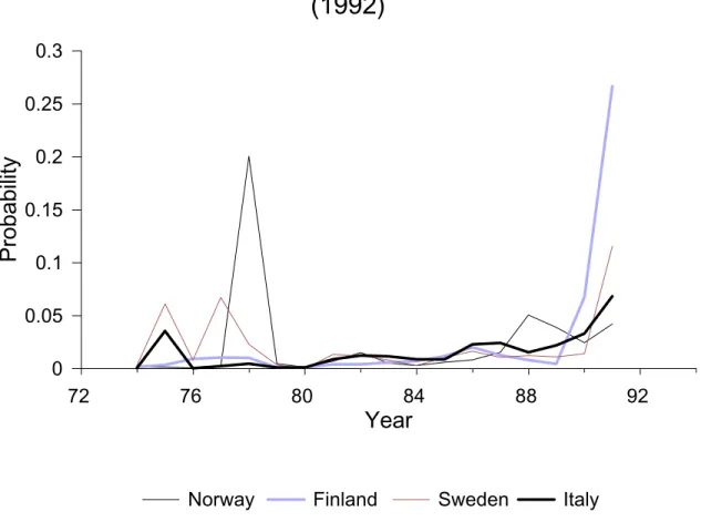
This Section examines the ability of the estimated Markov chain model to forecast exchange rate regime transitions. We focus on four recent prominent events. The transition from intermediate to °oating exchange rate regimes by Norway, Sweden, Finland, and Italy in 1992; by Thailand, Indonesia, Malaysia, and Korea in 1997; and by Mexico in late 1994; and the transition from intermediate to ¯xed exchange rate regime by Argentina in 1991.11

Consider ¯rst Figure 4 that contains the estimated probability of a transition from inter-mediate to °oating exchange rate regimes by Norway, Sweden, Finland, and Italy in 1992. This estimated probability corresponds to the ¯tted value of the model for this transition using as explanatory variables the rate of in°ation, trade openness, GDP growth, and re-serves/GDP (all lagged) and the coe±cients reported in Panel D in Table 3. The large spike for Norway in 1978 is associated with a severe recession in that year when output fell by around 4 percent on an annual basis. Notice that the transition probability rises for most

10_{Notice, however, that the Wald statistic of the null hypothesis that the coe±cients in both subsamples}

are the same is onlyW = 17:25: Since, this statistic is below the 5 percent critical value of a chi-square variable with 20 degrees of freedom, the hypothesis cannot be rejected. Given the small number of countries in each sample and the imprecision with which some of the coe±cients are estimated, it is possible that this result re°ects low test power.

11_{Our approach di®ers from currency crisis models in that we model a larger number of transitions rather}

than just a crisis event. Moreover, we consider changes in o±cial exchange rate regimes, not crises de¯ned as combinations of large movements in exchange rates and large movements in foreign exchange reserves. For a survey of the literature that attempts to predict currency crises, see Berg and Pattillo (1999).

countries after 1989, and in the case of Finland reaches 26 percent in the year prior to the change in regime. For the other countries the predicted probability for this transition rises to between 4 and 12 percent.

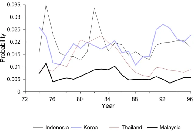
The model is not successful in predicting the exchange rate regime transitions in South East Asia in 1997 and in Mexico in the early 1990s.12 The estimated transition probabilities for Thailand, Indonesia, Malaysia, and Korea are plotted in Figure 5. Note that they do not change much in the year(s) prior to the crisis and in all cases are below 3 percent in 1996. In the case of Mexico (see Figure 6), the transition probability does increase somewhat prior to the transition, but is not very high by historical levels and reaches only roughly 5 percent in the year prior to the transition. There are two possible explanations for this result. First, annual data are likely to be too coarse to explain speculative attacks that take place in a matter of weeks. Second, as suggested by Burnside, Eichenbaum, and Rebelo (2001), current fundamentals might not be able to account for the Asian currency crisis if they were the result of future expected (as opposed to current) in°ation.

Finally, Figure 7 plots the probability of a transition from an intermediate to a ¯xed exchange rate regime in Argentina in 1991. Since in°ation is an important explanatory variable for this transition in emerging market economies, the transition probability rises after 1988 to reach roughly 30 percent in the year prior to the transition.

5

Conclusions

Results suggest that a fruitful way of obtaining some understanding of the distribution of exchange rate regimes is to try to explain transitions between regimes. Currency crisis models and the optimum currency area literature both imply that particular variables should help explain transitions. Estimates con¯rm that these variables have signi¯cant explanatory power, but case studies indicate that they do not always have a good forecasting power. When the sample includes all countries, high in°ation, and to a lesser extent low growth and low trade openness, tend to increase exits from the prevailing regime. This is consistent with currency crisis models (when considering the exits from intermediate or ¯xed regimes), but also withthe voluntary use of ¯xed or quasi-¯xed rates in exchange-rate-based stabilizations. In contrast, the level of reserves seems to have a less systematic impact. Reserves are signi¯cant in explaining transitions only for emerging market countries. This suggests that capital mobility may be lower for these economies than for the developed countries (that may have access to international capital markets even in a crisis).

What do these results have to say about hollowing out? Estimates suggest that low in°ation and sustained growth may be the key to making intermediate (and other) regimes sustainable. To the extent that in°ation decreases in emerging market economies (as it has done in many of them), and growth can be maintained, such regimes as soft pegs may be able to resist speculative attacks. It is in bad times, measured by bothvariables, that regimes are especially vulnerable.

We have been unable to get a proxy for capital mobility for a su±cient number of countries to include it as an explanatory variable. However, to the extent that increasing capital mobility makes emerging market economies resemble the advanced countries in our sample, the level of reserves should become less important as a determinant for exchange rate regime transitions.

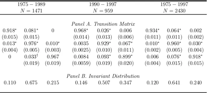
Table 1: Estimated Transition Matrix and Invariant Distribution All Countries

1975¡ 1989 1990¡ 1997 1975¡ 1997

N = 1471 N = 959 N = 2430

Panel A. Transition Matrix

0:918¤ 0:081¤ 0 0:968¤ 0:026¤ 0:006 0:934¤ 0:064¤ 0:002 (0:015) (0:015) (0:014) (0:013) (0:006) (0:011) (0:011) (0:002) 0:013¤ 0:976¤ 0:010¤ 0:0035 0:929¤ 0:067¤ 0:010¤ 0:960¤ 0:030¤ (0:004) (0:005) (0:003) (0:0025) (0:010) (0:011) (0:002) (0:005) (0:004) 0 0:033y 0:967 0:0084 0:093¤ 0:899¤ 0:006 0:076¤ 0:918¤ (0:019) (0:019) (0:0059) (0:019) (0:020) (0:004) (0:015) (0:015)

Panel B. Invariant Distribution

0:110 0:675 0:215 0:146 0:507 0:347 0:120 0:641 0:240

Notes: N is the number of observations. The superscripts¤ andy denote statistical signif-icance at the 5 and 10 percent levels, respectively. The ¯gures in parenthesis are standard errors.

Table 2: Estimated Transition Matrix and Invariant Distribution, Developed and Emerging Market Countries

(1975-1997)

Developed Emerging Markets

N = 478 N = 604

Panel A. Transition Matrix

0:857¤ 0:143 0 0:857¤ 0:143¤ 0 (0:093) (0:093) (0:054) (0:054) 0:003 0:972¤ 0:025¤ 0:008¤ 0:966¤ 0:025 (0:003) (0:009) (0:004) (0:008) (0:007) 0 0:029¤ 0:971¤ 0:016 0:078¤ 0:906¤ (0:014) (0:014) (0:015) (0:034) (0:036)

Panel B. Invariant Distribution

0:011 0:532 0:455 0:065 0:736 0:198

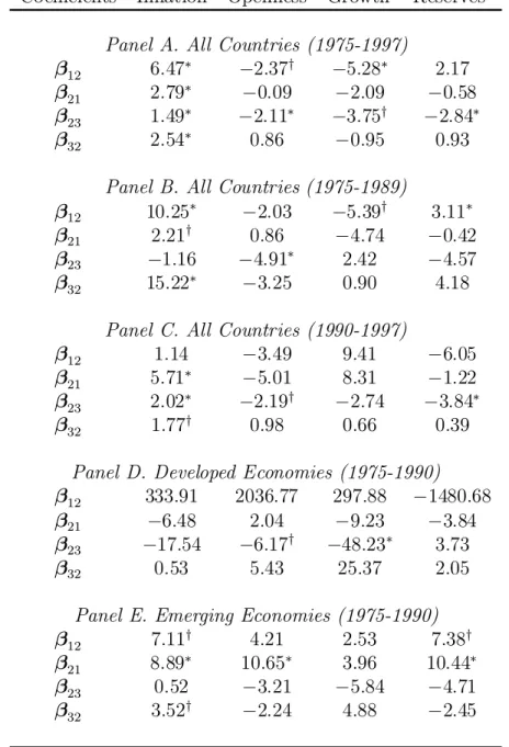
Table 3: Coe±cients of Explanatory Variables of Transition Probabilities Coe±cients In°ation Openness GrowthReserves

Panel A. All Countries (1975-1997)

¯12 6:47¤ ¡2:37y ¡5:28¤ 2:17

¯21 2:79¤ ¡0:09 ¡2:09 ¡0:58

¯₂₃ 1:49¤ ¡2:11¤ ¡3:75y ¡2:84¤ ¯32 2:54¤ 0:86 ¡0:95 0:93

Panel B. All Countries (1975-1989)

¯12 10:25¤ ¡2:03 ¡5:39y 3:11¤

¯21 2:21y 0:86 ¡4:74 ¡0:42

¯23 ¡1:16 ¡4:91¤ 2:42 ¡4:57

¯₃₂ 15:22¤ ¡3:25 0:90 4:18 Panel C. All Countries (1990-1997)

¯12 1:14 ¡3:49 9:41 ¡6:05

¯21 5:71¤ ¡5:01 8:31 ¡1:22

¯₂₃ 2:02¤ ¡2:19y ¡2:74 ¡3:84¤ ¯32 1:77y 0:98 0:66 0:39

Panel D. Developed Economies (1975-1990) ¯12 333:91 2036:77 297:88 ¡1480:68

¯21 ¡6:48 2:04 ¡9:23 ¡3:84

¯23 ¡17:54 ¡6:17y ¡48:23¤ 3:73

¯32 0:53 5:43 25:37 2:05

Panel E. Emerging Economies (1975-1990) ¯₁₂ 7:11y 4:21 2:53 7:38y ¯21 8:89¤ 10:65¤ 3:96 10:44¤

¯₂₃ 0:52 ¡3:21 ¡5:84 ¡4:71

¯32 3:52y ¡2:24 4:88 ¡2:45

Notes: see notes to Table 1. ¯_ij is a 5£ 1 vector of coe±cients on lagged annual in°ation, lagged openness to trade, lagged GDP growth, lagged foreign exchange reserves over GDP, and a constant term. The sample sizes for panels A, B, C, D, and E, are 2430, 1471, 959, 478, and 604, respectively.

References

[1] Andrews, D. W. K., and Fair, R. C., (1988), \Inference in Nonlinear Econometric Models withStructural Change," Review of Economic Studies 55: 615-640.

[2] Berg, A., and Pattillo, A., (1999), \Predicting Currency Crises: The Indicators Ap-proach and an Alternative," Journal of International Money and Finance, 18: 561-586. [3] Burnside, C., Eichenbaum, M., and Rebelo, S., (2001), \Propective De¯cits and the

Asian Currency Crisis," Journal of Political Economy 109: 1155-1197.

[4] Calvo, G., and Reinhart, C., (2002), \Fear of Floating," Quarterly Journal of Eco-nomics, 117: 379-408.

[5] Collins, S., (1996), \On Becoming More Flexible: Exchange Rate Regimes in Latin America and the Caribbean," Journal of Development Economics 51: 117-38.

[6] Edwards, S., (1996), \The Determinants of the Choice Between Fixed and Flexibile Exchange Rate Regimes," NBER Working Paper No. 5756.

[7] Eichengreen, B., (1994), International Monetary Arrangements for the 21st Century, Brookings: Washington, DC.

[8] Eichengreen, B., Masson, P., Savastano, M., and Sharma, S., (1999), \Transition Strate-gies and Nominal Anchors on the Road to Greater Exchange-Rate Flexibility," Essays in International Finance, No. 213. Princeton University, Princeton, NJ.

[9] Fischer, S., (2001), \Distinguished Lecture on Economics in Government { Exchange Rate Regimes: Is the Bipolar View Correct?," Journal of Economic Perspectives, 15: 3-24.

[10] Frankel, J.A., and Rose, A., (1998), \The Endogeneity of the Optimum Currency Area Criteria," NBER Working Paper No. 5700. National Bureau of Economic Research, Cambridge, MA.

[11] Ghosh, A. R., Gulde, A-M.,Ostry, J., and Wolf, H., (1997), \Does the Nominal Exchange Rate Matter?" NBER Working Paper No. 5874. National Bureau of Economic Research, Cambridge, MA.

[12] Hausman, R., Panizza, U., and Stein, E., (2000), \Why Do Countries Float the Way They Float?" unpublished, Inter-American Development Bank.

[13] Juhn, G., and Mauro P., (2001), \Determinants of Exchange Rate Regimes: A Simple Sensitivity Analysis," unpublished, IMF.

[14] Kremer, M., Onatski, A., and Stock, J., (2001), \Searching for Prosperity," NBER Working Paper No. 8250.

[15] Krugman, P., (1979), \A Model of Self-Ful¯lling Balance of Payments Crises," Journal of Money, Credit and Banking 11, 311-25.

[16] Levy Yeyati, E., and Sturzenegger, F., (1999), \Classifying Exchange Rate Regimes: Deeds vs. Words," Mimeo, available at http://www.utdt.edu/~ely

[17] Masson, P., (2001), \Exchange Rate Regime Transitions," Journal of Development Eco-nomics 64: 571-86.

[18] Masson, P., and Taylor, M., (1993), \Currency Unions: A Survey of the Issues," in Policy Issues in the Operation of Currency Unions, ed. P. Masson and M. Taylor, Cam-bridge: Cambridge University Press.

[19] Mundell, R., (1961), \A Theory of Optimum Currency Areas," American Economic Review 51(4): 657-65.

[20] Mussa, M., Masson, P. Swoboda, A, Jadresic, E., Mauro, P., and Berg, A., (2000), \Exchange Rate Regimes in an Increasingly Integrated World Economy," Occasional Paper 193 (Washington, IMF).

[21] Obstfeld, M., and Rogo® , K., (1995), \The Mirage of Fixed Exchange Rates," Journal of Economic Perspectives 9 (4): 73-96.

[22] Pesaran, M. H. and Ruge-Murcia, F. J., (1999), \Analysis of Exchange Rate Target Zones Using a Limited-Dependent Rational-Expectations Model withJumps," Journal of Business and Economics Statistics, 17: 50-66.

[23] Poirson, H., (2001), \How Do Countries Choose Their Exchange Rate Regime?," IMF Working Paper WP/01/46.

[24] Quah, Danny (1993), \Empirical Cross-Section Dynamics in Economic Growth," Euro-pean Economic Review 37: 426-34.

0 0.05 0.1 0.15 0.2 0.25 0.3

Probability

Year

Norway Finland Sweden Italy

Fig. 4: Italy and Nordic Countries

(1992)

0 0.005 0.01 0.015 0.02 0.025 0.03 0.035

Probability

Year

Indonesia Korea Thailand Malaysia

0.01 0.02 0.03 0.04 0.05 0.06 0.07 0.08

Probability

Year

Fig. 6: Mexico (1994)

0 0.05 0.1 0.15 0.2 0.25 0.3

Probability

Year

Fig. 7: Argentina (1991)