DYNAMICAL STUDY OF A SECOND ORDER DPCM TRANSMISSION SYSTEM MODELED BY A PIECE-WISE LINEAR FUNCTION
Texte intégral
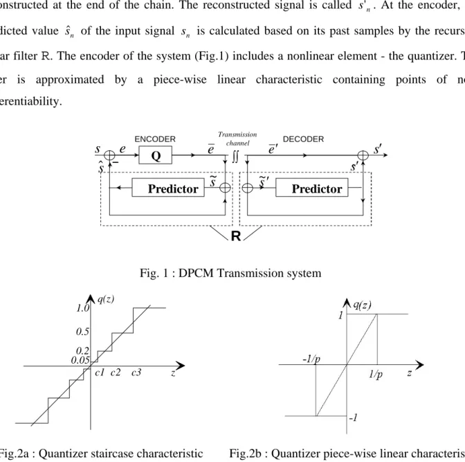
Figure
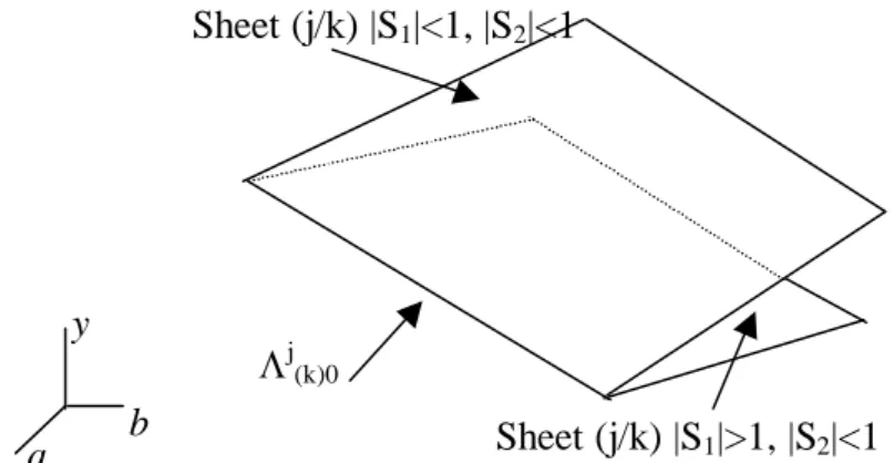
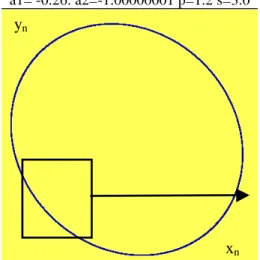
![Fig. 4 also gives the two dimensional non-linear projection of a three-dimensional qualitative representation [Taralova-Roux & Fournier-Prunaret, 1998]](https://thumb-eu.123doks.com/thumbv2/123doknet/8042545.269620/13.892.80.721.314.766/dimensional-projection-dimensional-qualitative-representation-taralova-fournier-prunaret.webp)
Documents relatifs
No calculators are to be used on this exam. Note: This examination consists of ten questions on one page. Give the first three terms only. a) What is an orthogonal matrix?
Démontre que tout entier impair peut s'écrire comme la différence des carrés de deux entiers naturels consécutifsb. Trouve tous les triplets
[r]
[r]
For otherwise, a small affine contraction orthogonal to the single pair of parallel minimal sup- port ~ines would reduce A (T1) without altering/~ (T1). Nor can it
These binomial theorems are evidently generalizations of corresponding theo- rems by NSrlund t (in the case where the intervals of differencing are identical).
Section 7 deals with kernels which include as a special case those possessing a derivative of fractional positive order (with respect to x).. On the
Estimates for the Fourier transform of the characteristic function of a convex set.. INGVAR SVENSSON University of Lund,
