HAL Id: hal-00259692
https://hal.archives-ouvertes.fr/hal-00259692
Submitted on 29 Feb 2008
HAL is a multi-disciplinary open access
archive for the deposit and dissemination of
sci-entific research documents, whether they are
pub-lished or not. The documents may come from
teaching and research institutions in France or
abroad, or from public or private research centers.
L’archive ouverte pluridisciplinaire HAL, est
destinée au dépôt et à la diffusion de documents
scientifiques de niveau recherche, publiés ou non,
émanant des établissements d’enseignement et de
recherche français ou étrangers, des laboratoires
publics ou privés.
Stijn Meganck, Philippe Leray, Bernard Manderick
To cite this version:
Stijn Meganck, Philippe Leray, Bernard Manderick. UnCaDo: Unsure Causal Discovery. Journées
Francophone sur les Réseaux Bayésiens, May 2008, Lyon, France. �hal-00259692�
Stijn Meganck
* —Philippe Leray
** —Bernard Manderick
** CoMo, Vrije Universiteit Brussel
Pleinlaan 2, 1050 Bruxelles, Belgique [email protected]
** LINA Computer Science Lab, Université de Nantes
2, rue de la Houssinière BP 92208, 44322 Nantes Cedex 03 [email protected]
RÉSUMÉ.La plupart des algorithmes pour découvrir des relations de causalité à partir de don-nées font l’hypothèse que ces dondon-nées reflètent parfaitement les (in)dépendances entre les va-riables étudiées. Cette hypothèse permet de retrouver le squelette théorique et le représentant de la classe d’équivalence de Markov du modèle dont sont réellement issues les données. Ce représentant est un graphe généralement partiellement orienté et sans circuit dont les arcs re-présentent des relations de causalité directe entre un ensemble de parents et le noeud enfant. Nous relachons cette première hypothèse en permettant d’obtenir initialement un graphe pou-vant contenir des arêtes "incertaines". Ces arêtes seront ensuite validées (et orientées) ou sup-primées lors de l’obtention de nouvelles données expérimentales. Nous présentons alors l’al-gorithme UnCaDo (UNsure CAusal DiscOvery) qui propose le plain d’expériences nécessaire pour obtenir suffisamment d’informations pour obtenir une structure complétement causale.
ABSTRACT.Most algorithms to learn causal relationships from data assume that the provided data perfectly mirrors the (in)dependencies in the system under study. This allows us to recover the correct dependence skeleton and the representative of the Markov equivalence class of Bayesian networks that models the data. This complete partially directed acyclic graph contains some directed links that represent a direct causal influence from parent to child. In this paper we relax the mentioned requirement by allowing unsure edges in the dependence skeleton. These unsure edges can then be validated and oriented or discarded by performing experiments. We present the UnCaDo (UNsure CAusal DiscOvery) algorithm which proposes a number of necessary experiments that need to be done to gain sufficient causal information to complete the graph.
MOTS-CLÉS :Réseau Bayésien Causal, Apprentissage de Structure.
KEYWORDS:Causal Bayesian Networks, Structure Learning.
1. Introduction
Learning causal relationships from data and modeling them is a challenging task. One well known technique for causal modeling is a causal Bayesian network (CBN), introduced by (Pearl, 2000). In a CBN each directed edge represents a direct causal influence from the parent to the child. For instance a directed edge C → E in a
CBN indicates that there exists at least one manipulation of C that would alter the distribution of the values of E given that all other variables are kept at certain constant values.
Learning the structure of Bayesian networks can be done from observational data. First the complete partially directed acyclic graph (CPDAG) is learned from data, and then a possible complete instantiation in the space of equivalent graphs defined by this CPDAG is chosen (Spirtes et al., 2000). It is impossible to follow the same strategy for CBNs, because there is only one true causal network that represents the underlying mechanisms, so only one of the graphs in the space of equivalent graphs is the correct one. Learning algorithms for which it is proven that they converge to the true CPDAG are PC proposed by (Spirtes et al., 2000), GES by (Chickering, 2003) and conservative PC by (Ramsey et al., 2006). (Shimizu et al., 2005) showed that when assumptions are made or prior knowledge is available about the underlying distribution of the data it is sometimes possible to recover the entire DAG structure from observational data.
To learn a CBN, experiments are needed because in most cases from observatio-nal data alone we can only learn up to Markov equivalence. Sometimes it is possible that the entire structure is discovered (e.g. there is only one member in the Markov equivalence class), however in general we can only learn a subset of the causal in-fluences. Several algorithms exist to learn CBNs based on experiments. For example, (Tong et al., 2001) and (Cooper et al., 1999) developed score-based techniques to learn a CBN from a mixture of experimental and observational data. In (Meganck et
al., 2006a) we proposed a decision theoretic based algorithm. (Eberhardt et al., 2005a)
performed a theoretical study on the lower bound of the worst case for the number of experiments to perform to recover the causal structure. All these results were based on performing structural interventions as experiments, i.e. randomization of a variable. Recently some work has been done on different types of interventions by (Eberhardt
et al., 2006) and (Eaton et al., 2007), but we will not go into detail in this paper.
We propose a constraint-based strategy to learn a causal Bayesian network using structural experiments in the case that observational data is not sufficient to learn all causal information and even insufficient to learn the correct skeleton of the network (i.e. imperfect data). We adapt an existing independence test and use this test to build a model able to represent unsure connections in a network. We then show how these unsure connections can be replaced either by a cause-effect relation or removed from the graph completely during the experiments phase.
The remainder of this paper is as follows. In the next section we provide notations and definitions needed in the remainder of this paper. Then we present our own
ap-proach and illustrate it on a toy example. We end with a conclusion and an overview of possible future work.
2. Preliminaries
In this section we introduce the basic elements needed in the rest of the paper. In this work uppercase letters are used to represent variables or sets of variables,
V = {X1, . . . , Xn}, while corresponding lowercase letters are used to represent their
instantiations, x1, x2and v is an instantiation of all Xi. P(Xi) is used to denote the
probability distribution over all possible values of variable Xi, while P(Xi = xi) is
used to denote the probability that variable Xiis equal to xi. Usually, P(xi) is used as
an abbreviation of P(Xi= xi). If two variables Xiand Xjare marginally dependent
or independent we denote this as(Xi 2Xj) and (Xi⊥⊥Xj) respectively. If the same
relations count conditioned on some set of variables Z we denote it as(Xi 2Xj|Z)
and(Xi⊥⊥Xj|Z) respectively.
Ch(Xi), Πi, N e(Xi), Desc(Xi) respectively denote the children, parents,
neigh-bors and descendants of variable Xiin a graph. Furthermore, πirepresents the values
of the parents of Xi.
Definition 1 A Bayesian network (BN) is a tuple,hV, G, P (Xi|Πi)i, with :
– V = {X1, . . . , Xn}, a set of observable random variables
– a directed acyclic graph (DAG) G, where each node represents a variable from
V
– conditional probability distributions (CPD) P(Xi|Πi) of each variable Xifrom V conditionally on its parents in the graph G such that the product of all P(Xi|Πi) is
a distribution.
As mentioned by (Pearl, 1988), several BNs can model the same independencies and the same probability distribution, we call such networks observationally (or Mar-kov) equivalent. A complete partially directed acyclic graph (CDPAG) is a represen-tation of all observationally equivalent BNs.
Definition 2 A partially directed acyclic graph (PDAG) is a graph containg both
di-rected and undidi-rected edges.
Definition 3 A complete partially directed acyclic graph CPDAG is a graph
consis-ting of directed and undirected edges. An edge A → B is directed if all BNs in the
equivalence class have an edge A→ B with the same directionality. An edge is
undi-rected if some have A→ B and some A ← B.
Definition 4 A Causal BN (CBN) is a Bayesian network in which the directed edges
parents-child tuple, while in a BN the directed edges only represent a probabilistic dependency, and not necessarily a causal one.
With an autonomous causal relation, we mean that each CPD P(Xi|Πi) represents
a stochastic assignment process by which the values of Xiare chosen only in response
to the values ofΠi. In other words, each variable Xj ∈ Πiis a direct cause of Xiand
no other variable is a direct cause of Xi. This is an approximation of how events are
physically related with their effects in the domain that is being modeled.
As (Murphy, 2001; Tong et al., 2001) and (Eberhardt et al., 2005b) have done, we will make some general assumptions about the domain being modeled.
Causal Markov condition : Assuming that B= hV, G, P (Xi|Πi)i is a causal
Baye-sian network and P is the probability distribution generated by B. As mentioned by (Spirtes et al., 2000), G and P satisfy the Causal Markov condition if and only if for every W in V , W is independent of V\(Desc(W ) ∪ ΠW)) given ΠW.
Faithful distribution : We assume the observed samples come from a distribution
which independence properties are exactly matched by those present in the cau-sal structure of a CBN.
Causal sufficiency : We assume that there are no unknown (latent) variables that
in-fluence the system under study.
3. UnCaDo
Some existing constraint-based structure learning methods can converge to the cor-rect CPDAG, however often the amount of data available does not permit this conver-gence. In this section we discuss our structural experiment strategy when the available observational data does not provide enough information to learn the correct CPDAG. We propose a constraint-based technique and assume causal sufficiency and the causal Markov property and that the samples come from a faithful distribution.
3.1. General description
The strategy of our approach consists of three phases. First an unsure dag, which is an undirected dependence structure, is learned using the observational data, that can include some unsure relations between nodes. In order to model these unsure relations we introduce a new type of edge, namely an unsure edge. Secondly all these unsure relations are removed from the graph by performing experiments in the system on the corresponding variables. In the final phase, possible remaining undirected edges are oriented.
3.2. Unsure independence test
The learning techniques we use are based on conditional (in)dependence tests. These tests need a certain amount of data in order to be reliable. If, for instance, not enough data was available then we can not draw a conclusion on the (in)dependence of two variables and thus are unsure whether an edge should be removed or added to the current graph. However most implementations of independence tests provide a standard answer in case there is not enough data. We propose an adapted independence test which in case there is not enough data or not enough evidence (this can be user dependent) for (in)dependence returns unsure as a result.
There are several ways to adapt existing independence tests, for instance : – Using χ2
, the number of data points has to be more than10∗(degree of freedom),
otherwise the test can not be performed reliably as mentioned by (Spirtes et al., 2000). In most implementations "no conditional independence" is returned as default, while in our case unsure would be returned.
– There can be an interval for the significance level used to return unsure. Traditio-nally tests are done using α= 0.05 significance level. We allow to set two parameters α1 and α2 with α1 > α2. We return independence if the test is significant for
si-gnificance level α2and unsure if it is significant for α1 and not for α2. For example
Unsure could be returned where the test is significant with α1 = 0.05, but no longer
insignificant for α2= 0.02.
3.3. Initial phase : unsure observational learning
We use the adapted independence test and modify the skeleton discovery phase of the PC algorithm in order to form an unsure graph.
The independence test used in PC corresponds to our adapted independence tests. The classic independence test returns either true or f alse, using our adaptation there is a third possible response unsure. When independence is found the edge between the two nodes is removed as usual, however when the relation between the two variables is unsure, we include a new type of edge o−?−o. In order to find sets to test for conditional
independence, arrows of type o−?−o are regarded as normal undirected edges.
Nodes in an unsure graph can have three graphical relations :
no edge : Xiand Xjare found to be independent conditional on some subset
(possi-bly the empty set).
edge Xio−oXj: Xiand Xjare dependent conditional on all subset of variables and
all conditional independence tests returned f alse. This corresponds to the tradi-tional undirected edge Xi− Xjand hence means either Xi← Xjor Xi→ Xj.
unsure edge Xio−?−oXj: we can not determine whether Xi and Xj are
in-dependence test returned unsure and none that return independent. This means that either Xi Xj, Xi→ Xjor Xi← Xj.
Note that as the number of data points N → ∞ the unsure edges will disappear,
since we will work with perfect data. In general however when there are unsure edges more data is needed to distinguish between independence and dependence, therefore we are in need of experiments.
3.4. Experimentation phase : resolving unsure edges
In this section we show how we can resolve unsure edges using experiments. We denote performing an experiment at variable Xiby exp(Xi).
In general if a variable Xiis experimented on and the distribution of another
va-riable Xj is affected by this experiment, we say that Xj varies with exp(Xi),
de-noted by exp(Xi) Xj. If there is no variation in the distribution of Xj we note exp(Xi) 6 Xj.
If we find when comparing the observational with the experimental data by condi-tioning the statistical test on the value of another set of variables Z that exp(Xi) Xjwe denote this as(exp(Xi) Xj)|Z, if conditioning on Z cuts the influence of
the experiment we denote it as(exp(Xi) 6 Xj)|Z. Note that conditioning on Z is
done when comparing the data, not during the experiment. A suitable blocking set Z is N e(Xj)\Xi, since this is sure to block all incoming paths into Xi.
We introduce additional notation to indicate that two nodes Xiand Xj are either
not connected or connected by an arc into Xj, we denote this by Xi−?−oXj, where
"−" indicates that there can be no arrow into Xi.
If we take a look at the simplest example, a graph existing of only two variables
Xiand Xjfor which our initial learning phase gives Xio−?−oXj. After performing an
experiment on Xiand studying the data we can conclude one of three things :
1) Xio−?−oXj
2) exp(Xi) Xj⇒ Xi→ Xj
3) exp(Xi) 6 Xj⇒ Xio−?− Xj
The first case happens if the added experiments still do not provide us with enough data to perform an independence test reliably. We can repeat the experiment until sufficient data is available or the test can be performed at our desired significance level. If no sufficient experiments can be performed the link remains Xio−?−oXj, this
possibility is a part of future work. The second case is the ideal one, in which we immediately find an answer for our problem.
In the third case, the only conclusion we can make is that Xi is not a cause of Xjand hence there is no arrow > into Xj. To solve this structure completely we still
need to perform an experiment on Xj. So in this case the results of performing an
4) exp(Xj) Xi+ (3)⇒ Xi← Xj
5) exp(Xj) 6 Xi+ (3)⇒ Xi Xj
In a general graph there can be more than one path between two nodes, and we need to take them into account in order to draw conclusions based on the results of the experiments.
Therefore we introduce the following definition :
Definition 5 A potentially directed path (p.d. path) in an unsure PDAG is a path
made of edges of types o−?−o, → and −?−o, with all arrowheads in the same direction.
A p.d. path from Xito Xjis denoted as Xi99K Xj.
If in a general unsure PDAG there is an edge Xio−?−oXj, the results of performing
an experiment at Xiare :
6) exp(Xi) Xj⇒ Xi 99K Xj, but since we want to find direct effects we need
to block all p.d. paths of length≥ 2 by a blocking set Z.
-(exp(Xi) Xj)|Z ⇒ Xi→ Xj
-(exp(Xi) 6 Xj)|Z ⇒ Xi Xj
7) exp(Xi) 6 Xj⇒ Xio−?− Xj
In the case that exp(Xi) 6 Xj we have to perform an experiment at Xj too. The
results of this experiment are :
8) exp(Xj) Xi+ (7)⇒ XiL99 Xj, but since we want to find direct effects we
need to block all p.d. paths of length≥ 2 by a blocking set Z.
-(exp(Xj) Xi)|Z + (7) ⇒ Xi← Xj
-(exp(Xj) 6 Xi)|Z + (7) ⇒ Xi Xj
9) exp(Xj) 6 Xi+ (7)⇒ Xi Xj
After these experiments all unsure edges Xio−?−oXj are transformed into either
directed edges or are removed from the graph.
It has to be noted that, like in the simplest example, the experiments only provide us with more data and that this still might not be enough to give a reliable answer for our statistical test. In this case the result of an experiment would leave the unsure edge and more experiments are needed until the test can be performed reliably.
3.5. Completion phase
At this point there are only the original undirected edges o−o and directed edges →
found by resolving unsure edges, we can hence use Steps 3 and 4 of PC to complete the current PDAG into a CPDAG. If not all edges are directed after this we need to
X1 X3 X2 X1 X3 X2 X1 X3 X2 ? X1 X3 X2 (a) (b) (c) (e) X1 X3 X2 ? (d)
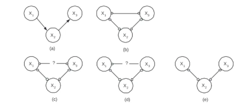
Figure 1. Simple example demonstrating the different steps in the UnCaDo algorithm.
perform another set of experiments. In order to complete this we use the MyCaDo algorithm we proposed in (Meganck et al., 2006a)
3.6. Complete Learning Algorithm
All the actions described above combine to form the Unsure Causal Discovery algorithm (UnCaDo). The complete algorithm is given in Algorithm 1. We define a couple of notions to simplify the notation. In an unsure graph N e(Xi) are all variables
connected to Xieither by a directed, undirected or unsure edge. Test of independence
in an unsure graph are performed using the unsure independence test we introduced above, in Algorithm 1 this test is referred to as the test of independence.
4. Toy Example
We demonstrate the different steps of the UnCaDo algorithm on a simple example. If the unsure independence test returns "unsure" for a test between Xiand Xj
condi-tioned on some set Z we note this as(Xi⊥?⊥Xj|Z). Assume the correct CBN is given
in Figure 1(a). The algorithm starts with a complete undirected graph shown in Figure 1(b). Assuming that the first ordered pair of variables that will be checked is(X1, X3)
and that we find the following (in)dependence information : –(X1 2X3)
–(X1⊥?⊥X3|X2)
This means that the edge X1o−oX3will be replaced by X1o−?−oX3, cfr. Figure 1(c). To
check for (in)dependence between the other sets of variables(X1, X2) and (X2, X3)
we regard the unsure edge X1o−?−oX3as being a normal undirected edge. This means
that we need to check for both the marginal as the conditional independence of these pairs. If the edge would be considered absent this might lead to missing necessary independence tests. Assume that we find the following independence information for
Algorithm 1 Adaptive learning of CBN for imperfect observational data and
experi-ments.
Require: A set of samples from a probability distribution faithful to a CBN P(V ).
Ensure: A CBN.
1) G is complete undirected graph over V . 2) Skeleton discovery of PC.
If any of the independence tests in this step of PC returned unsure, record the tuple(Xi, Xj) into P ossU nsEdg.
3) For each tuple(Xi, Xj) in P ossU nsEdg, if the edge Xi− Xjis still
present in G replace that edge by Xio−?−oXj.
4) For each unsure edge Xio−?−oXj,
Perform experiment at Xi,
If exp(Xi) Xj,
Find a (possibly empty) set of variables Z blocking all p.d. paths between
Xiand Xj.
If(exp(Xi) Xj)|Z then orient Xio−?−oXjas Xi→ Xj, else remove
the edge.
else replace Xio−?−oXjby Xio−?− Xj.
5) For each edge Xio−?− Xj,
Perform experiment at Xj,
If exp(Xj) Xi,
Find a (possibly empty) set of variables Z blocking all p.d. paths between
Xjand Xi.
If(exp(Xj) Xi)|Z then orient Xio−?− Xj as Xi← Xj, else remove
the edge.
else remove the edge.
6) Apply v-structure discovery and edge inference of PC. 7) Transform PDAG into CBN using the MyCaDo algorithm
(Meganck et al., 2006a).
–(X1 2X2) (X1 2X2|X3)
–(X2 2X3) (X2 2X3|X1)
So at the end of our non-experimental phase we end up with the structure given in Figure 1(c).
We now need to perform experiments in order to remove the unsure edge X1o−?− oX3. Assume we choose to perform an experiment on X1and gather all data Dexp.
There is a p.d. path X1o−oX2o−oX3so we have to compare all conditional distributions
to see whether there was an influence of exp(X1) at X3. Hence we find that :
and thus we can replace the edge X1o−?−oX3 by X1o−?− X3 as shown in Figure
1(d). Now we need to perform an experiment on X3, taking into account the p.d. path X3o−oX2o−oX1. We find that :
–(exp(X3) 6 X1|X2)
and we can remove the edge X1o−?− X3, leaving us the graph shown in Figure 1(e).
Now that all unsure edges are resolved we can use the orientation rules of the PC-algorithm, including the search for v-structures which in some cases will immediatly find the correct structure if enough data is available or we need to run the MyCaDo algorithm to complete the structure.
5. Conclusions and Future work
In this paper, we discussed learning the structure of a CBN. In general, without making assumption about the underlying distribution, the full causal structure can not be retrieved from observational data alone and hence experiments are needed.
We proposed an algorithm for situations when observational data is not suffi-cient to learn the correct skeleton of the network. Therefore we proposed an adapted (in)dependence test which can return unsure if the (in)dependence can not be detected reliably. We suggested to change the skeleton discovery phase of the PC algorithm in order to be able to include the adapted (in)dependence test. We proposed a new graph, an unsure graph, which can represent the results of the new discovery phase by means of unsure edges. We then showed how these unsure connections can be repla-ced either by a cause-effect relation or removed from the graph completely during an experimentation phase. The experiment strategy indicates which experiments need to be performed to transform the unsure DAG into a PDAG. Using a combination of the orientation rules of PC and, if necessary, some experiments, this PDAG can then be turned into the correct CBN.
We would like to extend these results to a setting with latent variables for which we will use our previous results proposed in (Meganck et al., 2006b).
For future research regarding learning with imperfect data we would like to study the case in which not all unsure edges can be removed. In this case the completion phase would regard them as being absent as not to make any false propagation mis-takes. We would like to study how we can use this to adapt our strategy to combine the experimentation and completion phase on a one-by-one basis instead of removing all the unsure edges first (Steps 4 and 5 in Algorithm 1) and then using one big completion phase (Steps 6 and 7 in Algorithm 1) as is presented in this article.
6. Bibliographie
Chickering D., « Optimal Structure Identification with Greedy Search », Journal of Machine
Cooper G., Yoo C., « Causal Discovery from a Mixture of Experimental and Observational Data », Proc. of Uncertainty in Artificial Intelligence, p. 116-125, 1999.
Eaton D., Murphy K., « Exact Bayesian structure learning from uncertain interventions », AI &
Statistics, p. 107-114, 2007.
Eberhardt F., Glymour C., Scheines R., N-1 Experiments Suffice to Determine the Causal Re-lations Among N Variables, Technical report, Carnegie Mellon University, 2005a. Eberhardt F., Glymour C., Scheines R., « On the Number of Experiments Sufficient and in the
Worst Case Necessary to Identify All Causal Relations Among N Variables », Proc. of the
21st Conference on Uncertainty in Artificial Intelligence, p. 178-184, 2005b.
Eberhardt F., Scheines R., « Interventions and Causal Inference », Philosophy of Science Assoc.
20th Biennial Mtg, 2006.
Meganck S., Leray P., Manderick B., « Learning Causal Bayesian Networks from Observa-tions and Experiments : A Decision Theoretic Approach », Proc. of Modelling Decisions in
Artificial Intelligence, MDAI 2006, p. 58-69, 2006a.
Meganck S., Maes S., Leray P., Manderick B., « Learning Semi-Markovian Causal Models using Experiments. », Proc. of The 3rd European Workshop on Probabilistic Graphical
Models., p. 195-206, 2006b.
Murphy K., Active Learning of Causal Bayes Net Structure, Technical report, Department of Computer Science, UC Berkeley, 2001.
Pearl J., Probabilistic Reasoning in Intelligent Systems, Morgan Kaufmann, 1988. Pearl J., Causality : Models, Reasoning and Inference, MIT Press, 2000.
Ramsey J., Zhang J., Spirtes P., « Adjacency-Faithfulness and Conservative Causal Inference »,
Proc. of the 22nd Conference on Uncertainty in Artificial Intelligence, p. 401-408, 2006.
Shimizu S., Hyvärinen A., Kano Y., Hoyer P. O., « Discovery of non-gaussian linear causal models using ICA », Proc. of the 21st Conference on Uncertainty in Artificial Intelligence, p. 526-533, 2005.
Spirtes P., Glymour C., Scheines R., Causation, Prediction and Search, MIT Press, 2000. Tong S., Koller D., « Active Learning for Structure in Bayesian Networks », Proc. of the 17th