Survey and analysis of kernel and userspace tracers on Linux : design, implementation, and overhead

Title

:

design, implementation, and overhead

Auteurs:

Authors

: Mohamad Gebai et Michel R. Dagenais

Date: 2018

Type:

Référence:

Citation

:

Gebai, M. & Dagenais, M. R. (2018). Survey and analysis of Kernel and userspace tracers on Linux : design, implementation, and overhead. ACM Computing

Surveys, 51(2), 26:1-26:33. doi:10.1145/3158644

Document en libre accès dans PolyPublie

Open Access document in PolyPublie

URL de PolyPublie:

PolyPublie URL: https://publications.polymtl.ca/3816/

Version: Version finale avant publication / Accepted version_{Révisé par les pairs / Refereed} Conditions d’utilisation:

Terms of Use: Tous droits réservés / All rights reserved

Document publié chez l’éditeur officiel

Document issued by the official publisher

Titre de la revue:

Journal Title: ACM Computing Surveys (vol. 51, no 2)

Maison d’édition:

Publisher: ACM

URL officiel:

Official URL: https://doi.org/10.1145/3158644

Mention légale:

Legal notice:

"© Dagenais | ACM 2018. This is the author's version of the work. It is posted here for your personal use. Not for redistribution. The definitive Version of Record was published in ACM Computing Surveys, https://doi.org/10.1145/3158644."

Ce fichier a été téléchargé à partir de PolyPublie, le dépôt institutionnel de Polytechnique Montréal

This file has been downloaded from PolyPublie, the institutional repository of Polytechnique Montréal

Survey and Analysis of Kernel and Userspace

Tracers on Linux: Design, Implementation, and

Overhead

Mohamad Gebai, Michel R. Dagenais Polytechnique Montreal

Abstract—As applications and operating systems are becoming more complex, the last decade has seen the rise of many tracing tools all across the software stack. This paper presents a hands-on comparishands-on of modern tracers hands-on Linux systems, both in user space and kernel space. The authors implement microbench-marks that not only quantify the overhead of different tracers, but also sample fine-grained metrics that unveil insights into the tracers’ internals and show the cause of each tracer’s overhead. Internal design choices and implementation particularities are discussed, which helps to understand the challenges of developing tracers. Furthermore, this analysis aims to help users choose and configure their tracers based on their specific requirements in order to reduce their overhead and get the most of out of them.

I. INTRODUCTION

Tracing has proved itself to be a robust and efficient approach to debugging and reverse-engineering complex systems. The past decade has seen the rise of many tracers across all layers of the software stack, and even at the hardware level [Intel CorporationIntel Corporation2016] [Sharma and DagenaisSharma and Dagenais2016a]. Some applications, such as Google Chrome, even provide tracers natively integrated within the product itself. Fundamentally, tracing is a sophisticated form of logging, where a software component, called the tracer, provides a framework that implements efficient and configurable logging. The most common use of logging by developers is done via the printf()function (or an equivalent), although this method is largely inefficient and limited. Tracers provide more flexible and robust approaches that can be easily maintained over time and usually add little overhead. Tracing is common in user applications, but is also widely used in the Linux kernel, which provides multiple tracing infrastructures. With complex online distributed systems, tracing becomes an efficient way of debugging problems whenever they arise. Although it is a problem that is often underestimated, the need for efficient and low-impact tracers is increasing, especially with modern parallel heterogeneous systems of ever increasing complexity. The Linux kernel contains over 1000 tracepoints and the volume of events that can be generated at runtime reinforces the need for low-impact tracers. In this article, we focus on the overhead that different tracers add to the traced applications, both at the user and kernel levels, on Linux systems. We start by establishing the nomenclature used in this work, and categorizing the many tools that have been gathered under the term “tracer”. We explain the differences

between them from the user point of view, we summarize the mechanisms used by each to perform its tasks, and we show key design and implementation decisions for each when relevant. We propose a microbenchmark that aims at providing reliable low-level and fine-grained metrics for an in-depth analysis and comparison.

In this work, we highlight the performance and the footprint of multiple tracers, as well as their underlying infrastructure. Many commercial and broadly-known tools rely on the tracing infrastructure variants studied here, and thus the overhead measured directly applies. The contribution of this paper is a deep dive into the design principles of modern tracers on Linux. This work tackles the problem of comparing tracers by measuring fine-grained and low-level performance metrics, so that the design choices made by the tracer developers, as well as the implementation and coding decisions, are taken into consideration when assessing the impact of a tracing tool on the traced system. Moreover, the contribution also encompasses a methodology for low-level benchmarking that unravels the real behavior of tracers, instead of using platform and micro-architecture emulators.

The rest of the paper is structured as follows: section II goes over previous work on tracers benchmarks, section III includes a reminder of key concepts required to understand the work presented and sets up the nomenclature used in this paper, section IV explains the mechanisms used in tracing, section V introduces the tracers and explains their internals when relevant, section VI explains the benchmarks, section VII shows the results of this work, section VIII concludes.

II. PREVIOUS WORK

Bitzes et al. [Bitzes and NowakBitzes and Nowak2014] studied the overhead of sampling using performance counters. However, their studies don’t address tracing in general. It also only focuses on the approaches for collecting hardware counters data and their performance overhead, rather than covering the internals of the tracers, or design and implementation choices. Sivakumar et al. [Sivakumar and Sundar RajanSivakumar and Sundar Rajan2010] measured the impact of the LTTng tracer, both in user and kernel space. The authors ran multiple known general benchmarks and reported the overhead that the tracer added. This approach helps to estimate the impact that LTTng may have on specific workloads but doesn’t quantify in detail the cost of the instrumentation,

or the cause of the overhead. Mihajlovic et al. [Mihajlovi´c, ˇZili´c, and GrossMihajlovi´c et al.2014] discuss their work to enable hardware tracing in virtual environments by modifying the ARM ISA emulation and show the overhead added by their approach. While the approach it presents is interesting, their approach relies on dynamic tracing which is a specific approach to tracing. Furthermore, it doesn’t cover or benchmark the fundamental work of tracers. Furthermore, no detailed comparison with other tracers is presented. Moore et al. [Moore, Cronk, London, and DongarraMoore et al.2001] reviewed performance analysis tools for MPI application. While they cover two of the tracers of this work, the work focuses primarily on the MPI framework, and doesn’t address kernel space tracing. The objective of the work also differs in that fundamental design choices of tracers with different scopes aren’t covered. In [GhodsGhods2016], the author explains and analyzes the internals of the Perf tool, mainly for sampling performance hardware counters. This work doesn’t cover comparisons with other tracing tools. The work of Desnoyers [DesnoyersDesnoyers2009] reports benchmarking results for LTTng and other tracers, albeit only showing the latency of recording an event, without presenting a detailed comparison with other tracers.

The infrastructures and frameworks presented in this article are often the basis for other commercial and more broadly-known monitoring and performance tools. For instance, the work by B. Gregg [??bgr2017] makes extensive use of Perf and eBPF. Flamegraphs are often generated by profiling ap-plications using Perf, although it is a profiler rather than a tracer. Another example is SysDig, which uses the tracepoint infrastructure to extract information from the kernel.

III. DEFINITIONS ANDNOMENCLATURE A. Definitions

This section serves as a reminder of some common terms in the world of tracing that are essential for understanding the rest of the paper.

Tracepoint: A tracepoint is a statement placed directly in the code of an application that provides a hook to invoke a probe. A tracepoint generally provides a way in which it can be enabled or disabled dynamically.

Probe: A probe is a function that is hooked to a tracepoint and is called whenever the tracepoint is encountered at run-time (if enabled). A probe usually performs a custom task and is either implemented by the tracer or by the user. Typically, a probe needs to be as small and fast as possible, to add as little overhead as possible and reduce the perturbation to the system.

Event: An event marks the encounter of a tracepoint at run-time. Depending on the kind of tracing, the event can have a logical meaning, such as a context switch, or can simply represent a location in the code, such as a function entry or exit. An event is punctual and has no duration, and is usually annotated with a timestamp.

Payload: An event typically holds a payload, which is additional information related to the event. For instance, the payload of a context switch may contain the identifiers of the

two tasks involved.

Ring buffer: A data structure that serves as a placeholder for events. When an event is recorded at run-time, the tracer’s probe is invoked. The probe records the encountered event by placing it in memory in the ring buffer (producer). At a later time, a consumer can read the contents of the ring buffer and report them to the user. When the data structure is full, the incoming events may either replace the oldest events (in a ring-like fashion) or they may be discarded until some events have been consumed from the buffer.

Atomic operation An atomic operation has the characteristic of being indivisible, which implies that intermediate values or intermediate states are invisible to concurrent operations. Atomic operations usually require support from the hardware or the operating system, and great care must be taken by the developer to guarantee atomicity. For instance, on x86 architectures, a mov instruction isn’t guaranteed to be atomic unless its operands are cache-aligned. Consider the case where one of the operands is stored across two pages: the mov instruction will require access to different pages (and poten-tially cause virtual address translations), making the operation divisible and non-atomic, as an intermediate unstable value can be visible if the operand is accessed by another instruction between these steps.

B. Nomenclature

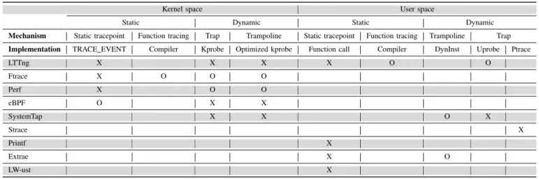
We previously defined a tracepoint as a location in an application where a probe can be hooked. This section starts by introducing the different mechanisms used for probe callback, as well as their implementations. A mechanism is a known theoretical approach as to how a callback can be implemented, but the actual implementation is left to the tracing infrastruc-ture. For instance, a trampoline is a mechanism that allows instrumentation at run-time, but the actual implementation of the trampoline is left to a tracing infrastructure such as DynInst or Kprobes. Similarly, a tool can support multiple mechanisms and allow its users to configure the mechanism to be used, depending on their needs. Tracers can then be built atop of these technologies to leverage their callback mechanisms, thus outsourcing this crucial part. Tracers can be built to support multiple callback mechanisms, for better flexibility and feature offerings. In summary, a tracer can use one or many callback implementations, which in turn implement one or many mechanisms. For instance, LTTng can use either TRACE_EVENT or Kprobes, and Kprobes can use either a trap or a trampoline.

We define a tracer as a tool that implements the following pattern: callback, serialize, write1_{. The output of a tracer is a}

trace, and efforts are dedicated to reducing as much as possible its overhead. On the other hand, tools such as eBPF and SystemTap fundamentally follow a different pattern: callback, compute, update. We refer to them as aggregators, since their work is often to collect and aggregate metrics in real time or in a live fashion, on the critical path of the applications, contrary to the post-mortem nature of trace analysis. To this end, they provide users with scripting capabilities and advanced

data structures (such as hashmaps) to implement aggregation methods to be executed upon certain events. As opposed to tracers, the output of aggregators is the result of the user-defined probe, which is typically a collection of metrics, an alert when a threshold is exceeded at runtime, and so on. They often neglect the timing aspect and don’t implicitly perform a clock read on each callback.

IV. CALLBACK MECHANISMS

This section introduces the different mechanisms used to instrument applications. The instrumentation can be static or dynamic, where the former is built into the binary at compile-time and tracepoint location is known in advance, and the latter is inserted at run-time at user-defined locations. This is not to be confused with dynamic tracing, which means that tracing can be turned on or off at run-time. Dynamic tracing can be supported for either static or dynamic instrumentation. To give better insights on how the mechanisms work, we cover their implementation in various technologies to show how they are effectively implemented and used.

A. Function instrumentation

Function instrumentation is a static instrumentation method that requires support from the compiler. The approach is to have each function call of an application prefaced by a call to a common tracing probe. In other words, the binary contains explicit calls to a specific routine upon each function entry (and exit in some cases). The implementation of this routine is left to the developer, or the tracer, and can implement tracing, profiling or any other monitoring feature.

GCCimplements this callback mechanism in various ways. For instance, the -pg flag will generate a binary where each function has the mcount routine call as a preamble [FrysingerFrysinger2016]:

$> echo "int main() {}" | gcc -pg -S -x c\ - -o /dev/stdout | grep mcount

call mcount

Since mcount is called at each function entry, additional efforts need to be put into its implementation to provide tracing at the lowest cost possible. Ftrace uses the mcount imple-mentation to trace kernel functions entries, and implements the mcount routine in platform-specific assembly. LTTng UST also uses this method for userspace tracing, albeit with the -finstrument-functions flag of gcc. Similarly to -pg, calls to specific routines are built into the binary not only at each function call entry, but also at function exit: $> echo "int main() {}" | gcc

-finstrument-functions -S -x c - -o \ /dev/stdout | grep cyg_profile

call __cyg_profile_func_enter

call __cyg_profile_func_exit

With the -finstrument-functions

flag, the instrumentation routines are called

__cyg_profile_func_enter() and

__cyg_profile_func_exit() for function entry and exit respectively.

B. Static Tracepoints

A tracepoint is a static instrumentation approach manually inserted directly in the application code by the developers.

Unlike regular function calls, tracepoint statements in the Linux kernel are optimized to have a minimal impact on performance. As the instrumentation is directly in the code and always built into the binary (unless the kernel is configured otherwise), great care must be taken to reduce the added overhead, especially when tracing is disabled, as is the case most of the time. The rest of this subsection discusses how this goal is achieved in the Linux kernel.

A disabled tracepoint has no effect and translates to a simple condition check for a branch [DesnoyersDesnoyers2016c] (in case it is enabled). To reduce the overhead for a disabled tracepoint, a hint is given to the compiler to make the tracepoint instructions far from the cache lines of the fast path (which is the regular code). In that way, the cache-friendliness of the fast path isn’t affected by the unexecuted code of the tracepoint. Furthermore, for kernel tracing, the tracepoint call is implemented as a C macro that translates to a branch over a function call. In that manner, the overhead of the function call and stack setup is avoided altogether.

Although the overhead impact of this approach is mini-mal in theory, it still requires reading from main memory the operand of the condition, to avoid the branch when the tracepoint is off. This adds non-negligible overhead as reading from memory not only is a slow process, but ul-timately affects the efficiency of the pipeline. To overcome this issue, the Immediate Value infrastructure was set in place [Desnoyers and DagenaisDesnoyers and Dagenais2008] by the LTTng project. This mechanism uses a constant value directly into the instruction’s operand. In that manner, no read from memory is required for the condition’s operand. A disassembly of the generated tracepoint code clearly shows the use of immediate values:

test %edx,%edx

jne [tracepoint tag]

When a tracepoint is turned on, the code is safely modified on the fly to change the value of the constant test check. Synchronization implications need to be taken into account for this process as the code resides in memory, and is shared amongst multiple CPUs, but copies may exist in instruction caches.

In the Linux kernel, static tracepoints are implemented as the TRACE_EVENT macro [RostedtRostedt2010], which allows developers to easily define a tracepoint that can be in-serted using the trace tracepoint name() function directly in the kernel code. Many of the current kernel tracers can interface to the TRACE_EVENT infrastructure by providing their own probes. This infrastructure also makes for an easy mechanism for a developer to implement their own tracer or aggregator.

For static tracepoints in user space, the LTTng tracer im-plements this mechanism with the same optimizations as for kernel space, reducing as much as possible the overhead added by the instrumentation.

C. Trap

Trap-based instrumentation is a mechanism to dynamically instrument an application at run-time. It relies on the operating system support for traps, which it exploits to insert and execute custom probes at virtually any location in the kernel or application code. In the Linux kernel, this mechanism is implemented by the Kprobe infrastructure, which uses a trap-based approach to dynamically hook into kernel code [Keniston J.Keniston J.2016]

[Mavinakayanahalli, Panchamukhi, Keniston, Keshavamurthy, and HiramatsuMavinakayanahalli et al.2006]. When a Kprobe is loaded and registered at a given instruction,

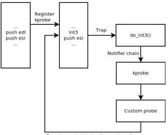
that instruction is copied and replaced with a breakpoint instruction (int3 on x86). When the breakpoint instruction is later executed by the CPU, the kernel’s breakpoint handler is invoked. It saves the state of the application (registers, stack, etc.) and gives control to the Kprobe infrastructure using the Linux notifier call chain, which ends up calling the tracing probe. Once this process completes and the trap has been handled, the copied instruction (that was replaced by the breakpoint) is finally executed and control continues normally at the call site. Image 1 shows this entire process. Kprobes also offer support for pre-handler and post-handler probes, as well as function return instrumentation (Kretprobe) which aren’t covered in this study.

Fig. 1: Trap-based callback mechanism with Kprobes A tracing infrastructure can be built atop Kprobes, where instead of manually inserting the trace tracepoint name() statement in the code at the call site, a Kprobe can be registered at the desired location at run-time. Tracers leverage this approach to connect their probe to a Kprobe instead of the TRACE_EVENT macro. In that manner, the callback mechanism is abstracted and only connecting the tracer’s probe to different backends provides more flexibility to the user. The resulting trace is identical to one that is generated using the

TRACE_EVENTmacro, but the callback mechanisms used to invoke the probes are different, which can have an impact on performance. When a Kprobe is unloaded, the breakpoint instruction is replaced with the original one, thus removing completely any trace of the instrumentation.

The Ptrace infrastructure in the kernel [Haardt and ColemanHaardt and Coleman1999]

[PadalaPadala2002] also uses traps to offer to userspace applications a mechanism to hook onto processes. It is important to note that, contrary to what its name suggests, Ptrace is not a tracer in itself, but rather an infrastructure provided by the Linux kernel for processes to monitor other processes. It allows a process to “hook” into another one and interrupt its execution, inspect its internal data, access its registers, etc. Many debuggers use Ptrace as a backend, including GDB.

D. Trampoline

Trampolines are a jump-based approach to dynamically patch or instrument an application at runtime. They provide a lower overhead alternative to trap-based mechanisms for the price of a more complex implementation. In more re-cent versions, the Linux kernel tries to optimize registered Kprobes using a jump-based trampoline instead of a costly breakpoint. The core of the optimization is to have a “detour” buffer (called the optimized region) to mimic the breakpoint approach [Keniston J.Keniston J.2016]. Instead of patching an instruction with a breakpoint instruction that triggers a trap, it is replaced by a simple jump to the optimized region. The jump-based approach starts by pushing the CPU’s registers onto the stack, jumps to a trampoline that acts as an in-termediate, which in turn jumps to the user-defined probe [HiramatsuHiramatsu2010]. When it completes execution, the process is reversed: the code jumps out of the optimized region, the registers are restored from the stack and execution of the original path continues. Note that not all loaded Kprobes use the trampoline approach, as it requires a set of conditions to be met (e.g., length of the instruction at the target location). If they aren’t, the kernel falls back to the breakpoint-based approach described previously.

V. THE TRACERS

This section introduces the tracers studied and benchmarked in this work. When relevant, details of the design and imple-mentation are provided for each tracer, and are later correlated with the results. Table I, presented at the end of this section, shows a summary of the tracers, as well as the mechanisms used by each (see section IV for an explanation of the mechanisms).

This work does not evaluate Dtrace

[Gregg and MauroGregg and Mauro2011] and Ktap [??kta2017]. The former is a proven tracer on Solaris and considered one of the pioneers in the field of tracing. However, it does not appear to be actively developed any more, with a total of 13 mailing list postings in the first half of 2017 on dtrace.org, its Linux port never reached the stability or broad usage of the Solaris port, and its strength lied more

in its flexibility and ease of use rather than its optimized performance and scalability [BrosseauBrosseau2017]. Ktap was an interesting lightweight dynamic tracing tool experiment based on bytecode, but was quickly superseded by eBPF which offers similar functionality but sharing a core infrastructure with other kernel subsystems.

A. Kernel tracers

1) None: The samples marked as ’None’ designate the baseline, which represents the system with all tracing disabled, effectively only benchmarking the instrumentation itself which is negligible (translates to a constant check as explained earlier).

2) Ftrace: Ftrace is a tracer included in the Linux kernel and shows insights into its internal behavior [RostedtRostedt2009a] [RostedtRostedt2016a] [RostedtRostedt2009b] by tracing all kernel function entries. It is controlled by a set of files in the debugfs pseudo-filesystem. Some of the main configurations include which “subtracer” to use, the size of the trace buffers and which clock source to use to timestamp the events. It is also possible to enable and disable specific events. Ftrace can be used in many ways: function tracing, tracepoints, system calls tracing, dynamic instrumentation and so on.

Function (and function graph) tracing reports the entry and exit of all functions at the kernel level. Ftrace can use the TRACE_EVENT infrastructure for static instrumentation tracing or the Kprobe infrastructure to dynamically hook into various parts of the kernel.

When tracing is enabled, the callback mechanism calls Ftrace’s probe which stores the events in a ring buffer. It is possible to configure Ftrace to either overwrite the oldest events or drop incoming events, once the ring buffer is full. It is interesting to note that the trace is kept in memory and not flushed to disk, and only made available upon reading the contents of the trace memory-backed file (it is possible to manually dump the contents of the trace file to disk). It is also possible to consume the ring buffer as it is written, through the trace_pipe file.

By default, Ftrace uses the local clock to timestamp the events it records. The local clock is a clock source that is CPU-local and is thus faster to read, but doesn’t provide any guarantee in terms of monotonicity and synchronization with the other CPUs’ clocks. It is, however, possible to configure Ftrace to use other clock sources, such as a global clock (which is system-wide), a logical counter or even architecture-specific clocks such as the TSC2 _{on x86.}

Ftrace limits the size of an event, including its payload, to that of a page. It uses per-CPU buffers, which avoids the need for synchronization of the buffer when tracing on multiple cores. Ftrace segments its ring buffers into pages and manipulates them individually. The ring buffer itself is a linked list of pages [RostedtRostedt2016b], and internal references are kept for bookkeeping. For instance, the tail page is a reference to the page into which the next event should be written, and the commit page is a reference to the page that

2_{TimeStamp Counter}

last finished a write. Although there can’t be simultaneous writers to the same page (per-CPU buffers), a writer can still be interrupted by another writer by the means of interrupts and NMIs. An example of that can be an event to be written into the buffer, from an interrupt handler context that was invoked while a write to the ring buffer was already happening, as shown in the following sequence:

Start writing

-> Interrupt raised Enter interrupt handler Start writing

Finish writing

Exit interrupt handler Finish writing

These nested writes require the tracer and its ring buffer to guarantee reentrancy in order to avoid data corruption and misbehavior. Note that there can be more than two levels of preemption (normal execution, interrupts, non-maskable interrupts, machine check exceptions, etc.). The way Ftrace ensures reentrancy is by dividing the writing process into three parts: reserving, writing, committing. The writing process starts by reserving a slot in memory in an atomic fashion, making it indivisible and thus guaranteeing reentrancy for this step. Only then can the writing into the reserved slot step begin. If a nested write occurs, it has to follow the same pattern, starting with a slot reservation. Since this can only happen after the preempted write has already completed its slot reservation (since it is indivisible), there can be no contention over the writing area, making the writing process safe. Once the nested write completes, it can commit which seals the writing transaction. The interrupted write can then complete its write and commit:

Reserve slot Start writing

-> Interrupt raised Enter interrupt handler Reserve slot

Start writing Finish writing

Exit interrupt handler Finish writing

By following this scheme, writing transactions appear as being atomic, in the sense that no two nested writes can write to the same slot in the buffer. When nested writes occur, some subtleties need to be implemented. For instance, the nested write cannot commit before the write it preempted. Until then, it is in the “pending commit” state. This is required since all events prior to the commit page have to be committed (the commit page actually points to the latest event that was committed, and masking its least significant bits gives the address of the page).

Furthermore, in order to consume tracing data, Ftrace keeps an additional page, called the reader page, which is not a part of the ring buffer. Rather, it is used as an interim to extract the trace data from the buffer. When a reader wants to consume trace data, the reader page is atomically swapped with the

head page. The head page is simply an internal reference to the page that should be read next. As this swap happens, the old reader page becomes part of the ring buffer, and the old head pagecan be safely consumed. This swapping happens in an atomic fashion using CAS (compare-and-swap) operations. After the swap happens, the head page pointer is updated to reference the next page to be read.

We explained earlier in this section that Ftrace manipulates pages individually in its ring buffer. Although this imple-mentation choice has benefits such as avoiding lazy memory allocations (and often a lazy TLB update), it also results in two main limitations: the size of an event (including its payload) is limited to the size of a page, and memory barriers are required at page boundaries. The former limitation is due to the fact that single pages are consumable. Consumption of the buffer can be done at page granularity, which implies that a single event cannot be stored across page boundaries. The latter limitation is less obvious; a page of the buffer can only be read once it is full. Thus, page management variables are required for internal bookkeeping, such as flagging a page as ready to be consumed. These variables are shared by the writer and any reader. To guarantee coherent ordering between buffer data and buffer management variables, memory barriers are required to ensure that a page is not flagged as full before its data is actually propagated to main memory.

3) LTTng: LTTng was created in 2006

[Desnoyers and DagenaisDesnoyers and Dagenais2006b]

[DesnoyersDesnoyers2009] [Desnoyers and DagenaisDesnoyers and Dagenais2009], around the same time as Ftrace and thus both tracers share

many similarities design-wise. However, LTTng isn’t part of the mainline Linux kernel and is rather deployed as a group of loadable kernel modules for the kernel tracing part, and a userspace component for tracing management and trace consumption (as opposed to Ftrace’s debugfs interface). LTTng was designed and implemented with the objective of minimal performance impact [Desnoyers and DagenaisDesnoyers and Dagenais2006a] while being fully-reentrant, interrupt-safe and NMI-safe. Similarly to Ftrace, LTTng uses per-CPU variables and buffers to avoid concurrent writes and the need for synchronization. Reentrancy is guaranteed by the means of atomic slot reservation using local CAS (Compare-And-Swap) to permit nested writes [Desnoyers and DagenaisDesnoyers and Dagenais2012], similarly to what was explained in section V-A2. Image 2 shows how having (local) atomic slot reservation guarantees reentrancy. As the figure shows, in sub-buffer 1 of buffer 0 (on CPU 0), a first event was written into the buffer. A slot was reserved after it for writing, but the process was interrupted midway through by another write. We see that this nested write completes successfully, and doesn’t affect the end result of the interrupted write, as its slot is already reserved.

The low-overhead requirements of the LTTng project have lead to the creation of local atomic operations in the Linux kernel [DesnoyersDesnoyers2016b], which aim to provide a lower performance cost than regular atomic operations, by leveraging the fact that some data is CPU-local (that is, data

Fig. 2: Anatomy of LTTng’s sub-buffers

that won’t be accessed by another CPU). When that is the case, atomic operations accessing local-only data don’t require the use of the LOCK prefix (which locks the memory bus) or memory barriers to ensure read coherency between CPUs, which leads to local atomic operations. This performance improvement comes at the cost of a higher usage complexity, and care is needed when accessing the data from other CPUs due to weak ordering. It is worth mentioning that local atomic operations disable preemption around the call site to avoid CPU migration when accessing local variables from a process context (as opposed to interrupt context). Ftrace also makes use of local atomic operations.

To guarantee wait-free reads of tracing management variables (such as enabling/disabling tracing, filters to be applied, etc.), LTTng uses RCU3

for the synchronization of concurrent accesses [McKenney and SlingwineMcKenney and Slingwine1998] [Desnoyers and DagenaisDesnoyers and Dagenais2010]. Since writes to these variables are rare, but reads are abundant and concurrent, RCU is ideal for such an access pattern since it avoids all waiting on the reader side.

Contrary to Ftrace, LTTng doesn’t use pages as the finest-grained entity for ring buffer management. Instead, it uses per-CPU sub-buffers. The advantage of this approach is that the size of an event can be greater than the size of a page, and the performance hit of memory barriers is better amortized (barriers are only required at sub-buffer boundaries instead of page boundaries). Sub-buffer boundaries require memory barriers mainly to guarantee in-order memory writes to the sub-buffer data and its management variables. In other words, out-of-order memory accesses to sub-buffer data and the sub-buffer management variables can result in incoherent perception from the reader’s side, where a sub-buffer can be

flagged as ready to be read while the tracing data hasn’t been propagated to memory yet. It is interesting to note that the impact of memory barriers is negligible on x86 64. Since the architecture guarantees Total Store Ordering (TSO) between CPUs [Hennessy and PattersonHennessy and Patterson2011], write memory barriers do not actually create a fence but resolve to nops and simply avoid instructions reordering at compile-time. On architectures with other memory orderings such as ARM, the use of memory barriers at sub-buffer boundaries (page boundaries for Ftrace) has a larger impact on the overhead.

4) LTTng-kprobe: We introduce LTTng-kprobe as a stan-dalone tracer for simplicity purposes. In reality, it is sim-ply the LTTng tracer configured to use Kprobes instead of TRACE_EVENT for probe callback. Other than the callback mechanism, there are no differences for the probes or the ring buffer, and the same internals and guarantees as LTTng are valid for this tracer.Comparing the benchmark results between LTTng-kprobe and LTTng will highlight the impact of using Kprobes instead of TRACE_EVENT. This comparison can help developers assess the overhead of Kprobes-based tracers in their applications when low overhead is key.

5) Perf: Perf is a performance monitoring tool integrated into the mainline kernel. Its use case is typically different than that of Ftrace or LTTng. Perf is targeted for sampling and profiling applications, although it can interface with the tra-cepoint infrastructure within the kernel and record tratra-cepoints (including system calls). Perf can also gather hardware-level PMU4 _{such as different level of cache misses, TLB misses,}

CPU cycles, missed branch predictions, and so on. Contrary to Ftrace, Perf’s monitoring scope is restricted to a single process. The events and counters reported by Perf are those which occurred within the context of the traced process and thus have been accounted for it. This property makes Perf more suited to analyze the behavior of a given program and can help answer practical questions such as cache-friendliness of the code, or the amount of time spent in each function.

The Perf tool itself is built on top of the kernel’s perf_events subsystem [GhodsGhods2016] which is the part that actually implements the tracing, profiling and sam-pling functionalities. Perf can also use Ftrace’s architecture to hook to tracepoints, and trace similarly to Ftrace and LTTng. Perf_events internally uses a ring buffer which can be mapped to userspace to be consumed. Through the perf_event_open()system call, a userspace process can obtain a file descriptor on the metric/counter it wants to measure. The file descriptor can then be mmap()’d and accessed from the userspace process’s memory space.

6) eBPF: eBPF has evolved from the Berke-ley Packet Filter [Schulist J.Schulist J.2016] [McCanne and JacobsonMcCanne and Jacobson1993] to a standalone monitoring tool included in the Linux kernel. It allows users to write programs (similarly to probes) which can be dynamically inserted at any location in the kernel using Kprobes (section IV-C). eBPF programs are compiled to bytecode which is interpreted and executed by the kernel

4_{Performance Monitoring Units}

in a limited context to ensure security. The kernel also supports just-in-time compilation for sections of the generated bytecode [Sharma and DagenaisSharma and Dagenais2016b]. It is important to note that eBPF isn’t a tracer, as it doesn’t follow the callback, serialize, write scheme, but rather an aggregator. The eBPF interpreter provides data structures to its users, such as simple arrays and hashmaps, which makes it a great tool for aggregation, bookkeeping, and live monitoring. As eBPF provides arrays that can be shared from the kernel space to user space, a tracer-like behavior can be implemented. For the purpose of this study, we wrote a minimal eBPF program that samples the clock and writes a data structure holding a timestamp and a payload to an eBPF array. We hook this program to the same static tracepoint used for benchmarking other tracers using Kprobes. Although the data is never read, this program simulates the behavior of a tracer, making its benchmarking relevant for this study. As of version 4.7, the Linux kernel supports eBPF tracing, which hooks directly into the TRACEPOINT infrastructure. The same eBPF program was then ran on a 4.12 Linux kernel, with the only difference being a direct hook onto kernel tracepoints instead of going through Kprobes.

7) SystemTap: SystemTap is similar to eBPF (section V-A6) as it provides a simple language to write probes for aggregation and live monitoring [Prasad, Cohen, Eigler, Hunt, Keniston, and ChenPrasad et al.2005]. SystemTap provides an easy scripting language for users to create custom probes to monitor their systems. The users can provide kernel or userspace symbols to hook on. SystemTap programs are then translated to C code and compiled into a loadable kernel module [EiglerEigler2006]. Once loaded, the module dynamically inserts the probe into the kernel’s code using Kprobes. Similarly to eBPF, since SystemTap follows the callback, compute, update pattern, it is, in fact, an aggregator rather than a tracer. However, for the purposes of our work, a tracing behavior can be simulated by implementing a probe that samples the time and writes the value along with a constant payload to an internal array.

8) Strace: Strace is a tool for

sys-tem calls tracing [KerriskKerrisk2010]

[Johnson and TroanJohnson and Troan2004]. Using Ptrace (section IV-C), it hooks into a process and intercepts all its system calls, along with their arguments. The result is written to a file descriptor for later analysis. Due to the heavy trap mechanism, along with the scheduling costs (as multiple processes are involved, the monitored and the monitoring), Strace typically adds a large overhead which doesn’t usually suit production environments. Other tracers, such as LTTng and Ftrace, can provide the same information using different tracing mechanisms.

9) SysDig: SysDig [Selij and van den HaakSelij and van den Haak2014] is a modern commercial tool used for monitoring systems.

It covers a wide range of applications, from containers, to web services, etc. SysDig also allows users to write Chisels [??chi2017], which are lua scripts capable of custom analysis similar to eBPF and SystemTap. SysDig leverages the TRACEPOINT infrastructure in the kernel, which was introduced by the LTTng project, to hook onto available

tracepoints and provide system and application monitoring. Upon loading, the SysDig kernel modules register to context switch and system calls events. The work presented in this article does not cover SysDig for two main reasons. Primarily, SysDig doesn’t allow the users to control the kernel tracing part of the product, and this aspect is only used to gather a few metrics about the monitored applications, such as reads, writes and CPU usage. Moreover, SysDig doesn’t follow the callback, serialize, write pattern, but rather uses tracepoints for on-the-fly metric gathering. Finally, as SysDig uses the same underlying infrastructure as LTTng and Ftrace, the overhead of SysDig is implicitly covered when studying the TRACEPOINTinfrastructure.

B. Userspace tracers

1) Printf: Printf() is a rudimentary form of tracing, but is the easiest to use. It uses a string as input as well as some variables for pretty-printing. Printf() uses an internal buffer to store the data before it is flushed to a file descriptor. Thus, we can implement a basic tracer using printf() by sampling the time and printing it along with a payload into printf()’s internal buffer. This satisfies the definition of a tracer given in section III-A.

Glibc’s implementation of printf() is thread-safe [PeekPeek1996], although multiple threads within the same application share the same global buffer for the output stream. Printf() uses an internal lock to protect the output buffer and avoid corruption on contention. However, reentrancy is not guaranteed, and calling printf() from different contexts (such as from a signal handler that interrupts printf()) might have unexpected results.

2) LTTng UST: LTTng UST (UserSpace Tracer) [Blunck, Desnoyers, and FournierBlunck et al.2009]

is a port to userspace of LTTng (section V-A3). Although they are independent, both tracers share the same design, using a ring buffer to store the trace [Fournier, Desnoyers, and DagenaisFournier et al.2009], RCU mechanism for data structure synchronization and atomic operations for reentrancy. To this effect, the RCU mechanism was ported to userspace as well, creating the URCU (Userspace Read-Copy-Update) project

[Desnoyers, McKenney, Stern, Dagenais, and WalpoleDesnoyers et al.2012]. All programs to be traced with LTTng UST should be linked

against the library, as well as libust (the tracing library). Similarly to its kernel counterpart, LTTng UST was designed and implemented to perform tracing at low cost, while guaranteeing reentrancy, interrupt-safety, signal-safety, etc. No tracing data is copied and no system calls are invoked by the tracer, removing the typical sources of overhead.

3) LTTng using tracef(): Since part of printf()’s la-tency is split between pretty printing the input and storing to an internal buffer, we added LTTng’s tracef() function for a more equitable/fair comparison. Tracef() is a function that combines, from the developer’s point of view, LTTng’s tracer and printf(). Instead of implementing actual tracepoints that can be called within the code, tracef() generates a lttng_ust_tracef event which holds as payload a

pretty-printed string similarly to printf(). In that manner, LTTng’s internal ring buffer mechanism is used, while includ-ing the cost of pretty printinclud-ing for a more equitable comparison with printf(). In that way, we compare more accurately the actual serialization to a ring buffer between LTTng and printf().

Since tracef() uses LTTng’s internals and only affects the serialization part, the same guarantees as tracing using regular tracepoints apply, such as reentrancy, thread-safety, interrupt-safety and so on.

4) Extrae: Extrae is a tracer developed at the Barcelona Supercomputing Center (BSC) as part of a tracing and analysis infrastructure for high-performance computing. It has complementary software such as Paraver [Pillet, Labarta, Cortes, and GironaPillet et al.1995] for trace visualization and analysis. In this paper, we focus exclusively on the tracing part. The tracer supports many mechanisms for both static and dynamic instrumentation, as shown in Table I. It also uses LD_PRELOAD to intercept MPI library calls at runtime and instrument them. In addition, Extrae supports sampling hardware counters through the PAPI interface [Terpstra, Jagode, You, and DongarraTerpstra et al.2010], and other features which aren’t covered in this study as they are beyond the scope of tracing [??ext2016]. Extrae also uses internal per-thread buffers to store the data on the fly. Static tracepoints have limited features: only one type of tracepoint exists which is called Extrae_event, having two fields as a payload. The fields are a pair of integers, the first one being a number representing the type of event that occurred, and the other flags either a function entry or exit. This provides less flexibility to the user to create and use custom tracepoints with variable payloads.

5) VampirTrace: VampirTrace is

a high-performance computing tracer

[Kn¨upfer, Brunst, Doleschal, Jurenz, Lieber, Mickler, M¨uller, and NagelKn¨upfer et al.2008] [M¨uller, Kn¨upfer, Jurenz, Lieber, Brunst, Mix, and NagelM¨uller et al.2007]

[Sch¨one, Tsch¨uter, Ilsche, and HackenbergSch¨one et al.2010], with the ability to interface with large-scale computing frameworks such as MPI. Similarly to Extrae, it offers many ways to instrument applications, either statically or dynamically. For static tracing, VampirTrace uses a different approach and relies on the developer to define the sections of code to be analyzed. When tracing of a section is disabled through a delimiter, an event is generated and written to the buffer. VampirTrace uses per-thread buffers to avoid synchronization and maintain scalability. The microbenchmark of this paper for VampirTrace consists of a tight loop that enables and disables tracing. This implementation defines an empty section to trace, but generates an event on each loop, due to disabling tracing on each loop so that a behavior similar to other tracers is achieved.

6) Lightweight UST: Lightweight UST (LW-ust) is an in-house minimal tracer built for the purpose of this study. It targets the fastest possible naive tracing implementation, at the cost of actual usability, reentrancy, and thread-safeness. The purpose of this tracer is to show a baseline of how fast tracing can be achieved, which is a simple clock read and a copy into an internal buffer. LW-ust uses per-CPU circular buffers to

write data, which are cache line-aligned to avoid false sharing. The data copied into the buffer is simply an integer referring to the tracepoint type, a timestamp (using clock_gettime(), similarly to other tracers) as well as another integer as the tracepoint payload. No effort is made towards reentrancy or thread-safety, and thus data integrity is not guaranteed. Although LW-ust can not be used on production systems, it is still interesting to benchmark it as it provides a lower bound on the impact of a tracer.

VI. BENCHMARKING A. Objectives

The objective of this study is to quantify the overhead added by tracing, taking into consideration different callback mechanisms, internal tracers’ architectures, and the guarantees they provide. We focus on the cost of individual tracepoints, rather than analyzing the impact on more general workloads. By analyzing the results, we hope to help the users configure the tracers to adapt them for their specific use cases when low overhead is a requirement in production systems.

B. Approach

1) Overview: We start by explaining our benchmark related to kernel tracing as well as the metrics we measured. Our objective is to measure the cost of tracing an event using the different tracers. To be able to get this metric with the best possible precision, two conditions have to be met: first, all tracers must be running in the overwrite mode. That way, we guarantee that all tracepoints are executed, even when the internal ring buffers are full, as opposed to benchmarking a test and nop operation (testing the buffer size and jumping over the tracepoint if the buffer is full). Secondly, when possible, we launch tracers in a producer-only mode. This requirement helps to cancel outside noise that might interfere with the benchmarking. In our case, the consumer process might preempt the traced process, or the action of writing to the disk or the network might also interfere in some way with the producer. Although we are only measuring isolated tracepoints, and preemption doesn’t directly affect the duration of executing a tracepoint, it still, however, impacts the duration of a tracepoint since it might invalidate caches (including the TLB for which misses are particularly expensive).

The actual measurement is done in a microbenchmark which is simply a tight loop executing a tracepoint call. The payload of the event is 4 bytes. The microbenchmark is implemented in a kernel module to avoid the overhead of switching between user and kernel spaces. A single ioctl() call to the module (via the sysfs pseudo-filesystem) triggers the benchmark and blocks until its completion.

The time is measured prior and after the call at the nanosecond granularity. We point out that there is no system call for reading the time since the benchmark is already running in kernel space (although some clock access functions can be used in user space to avoid a system call, such as the mono-tonic clock). Hardware performance counters are also read before and after the tracepoint, allowing us to track specific metrics that give insight into each kernel’s implementation.

The benefit of sampling many hardware counters in a single run, instead of sampling a single counter across many runs (to reduce the impact of these samplings) is that it is possible a posteriori to make correlations between many metrics for a single recorded event. For instance, we can verify if the slow path (given by sampling the number of instructions) can be further optimized by reducing cache misses (given by sampling the number of cache misses). Due to hardware limitations, only four hardware counters can be sampled at a time. Thus, two runs of the benchmark are executed, each sampling different counters. Furthermore, in order to avoid interruption while the tracepoint is executing, which would interfere with the measurements, we disable interrupts before each call and enable them after. Since this approach doesn’t disable NMIs (which are, by definition, non-maskable), we read the NMI count prior to and after each tracepoint call, discarding the result values in case an NMI is detected. Algorithm 1 shows the pseudo-code of the benchmark. The results shown in this paper are gathered by running the tight loop 5000 times in a steady state for each benchmark run. For scalability tests, the tight loop iterates 5000 times per core (in parallel) in a steady state for each benchmark run.

Algorithm 1: Pseudo-code of the kernel tracer benchmark Input: numberOf Loops

Output: ArrayOf Results payload = (int32 t) 0; results = allocateArray(); i = 0; while i != numberOfLoops do disableInterrupts(); numberNMI = getNumberNMI(); readPMU(metric1 start); readPMU(metric2 start); readPMU(metric3 start); readPMU(metric4 start); start time = gettime(); tracepoint(payload); end time = gettime(); readPMU(metric1 end); readPMU(metric2 end); readPMU(metric3 end); readPMU(metric4 end); enableInterrupts();

if numberNMI == getNumberNMI() then results[i].duration = end time - start time; results[i].metric1 = metric1 end - metric1 start; results[i].metric2 = metric2 end - metric2 start; results[i].metric3 = metric3 end - metric3 start; results[i].metric4 = metric4 end - metric4 start; i++;

end end

return results;

The final results array is then dumped in a CSV (Comma-Separated Value) file, which is used to generate the graphs shown in section VII. The same algorithm is used for both kernel and user space.

Benchmarking system calls and analyzing the results require a different methodology than regular tracepoints. The added cost of the actual system call, as well as the fact that the Linux

TABLE I: Callback mechanisms for kernel and userspace tracers

’X’ indicates that a callback mechanism is supported by the tracer and is covered in this work ’O’ indicates that the mechanism is supported by the tracer but wasn’t benchmarked in this work

Kernel space User space

Static Dynamic Static Dynamic

Mechanism Static tracepoint Function tracing Trap Trampoline Static tracepoint Function tracing Trampoline Trap Implementation TRACE EVENT Compiler Kprobe Optimized kprobe Function call Compiler DynInst Uprobe Ptrace

LTTng X X X X O O Ftrace X O O O Perf X O O eBPF O X X SystemTap X X O X Strace X Printf X Extrae X O LW-ust X

kernel automatically instruments system call entry and exit, make getting fine-grained metrics about the tracing mechanism only more difficult. Since actual work is done by the system call, PMU counters values aren’t representative of the tracing mechanism solely, but also include the system call’s execution. In addition, the CPU transitions from user mode to kernel mode through a trap that represents the actual kernel invoca-tion. This is a relatively costly process, since it requires saving the state of the stack, registers, and switching CPU rings [Tanenbaum and BosTanenbaum and Bos2014]. This proce-dure is therefore implicitly accounted for the tracepoint in the benchmark. The analysis and benchmarking of system calls are thus done at a higher level, with coarse-grained results. It is worth mentioning that system calls tracing is a subset of kernel tracing, which we presented in the previous section. In other words, writing to the ring buffer is done in the same fashion, and only serializing the payload differs from a regular tracepoint.

In order to reduce as much as possible the duration of the system call’s actual work and get samples that are as close as possible to the cost of instrumentation solely, we benchmarked an empty ioctl() system call. For the purpose of this work, we wrote a kernel module that exports an entry in procfs. We implemented its ioctl() function as an empty function, such that calling ioctl() on the file descriptor returns as quickly as possible, and ends up being only the tracing instructions and a CPU context switch to kernel space and back.

2) Test setup: We ran the benchmarks on an Intel i7-3770 CPU running at a 3.40 GHz frequency with 16 GB of RAM, running a 4.5.0 vanilla Linux kernel, and a 4.7.0 Linux kernel for eBPF tracing (as it is the first version that introduced built-in eBPF tracing). We built manually the following software: LTTng from its 2.9-rc1 branch, SystemTap from its master branch at version 3.0/0.163, and Extrae at version 3.3.0, and VampirTrace at version 5.14.4.

3) Configuration: Benchmarking at such a low granularity proves to be a tedious task relatively to higher level

benchmarks [Kalibera and JonesKalibera and Jones2013]. Optimizations, both at the operating system level as well as the hardware level, can interfere greatly with the results. Not only are the results biased, but reproducibility of the results is also affected. For instance, dynamically adjustable CPU frequency has a direct impact on the latency of a tracepoint. In order to have the most control over the environment, we disabled the following features at the hardware level: hyperthreading, C-states, dynamic frequency and Turbo Boost.

Furthermore, we configured the tracers to have as much of the same behavior as possible to obtain relatively fair results. For instance, as shown in section V-A2, Ftrace uses a CPU-local clock source to sample the time, whereas LTTng uses a global clock. At the nanosecond scale, as we are benchmarking, this behavioral difference can have a major impact on the results. We configured Ftrace to use the global clock so that the same time sampling mechanism is used by all tracers. We configured LTTng to use 2 sub-buffers per CPU buffer, each of 8 KB, and Ftrace to use a 16 KB buffer per CPU (same ring buffer size). We also configured LTTng to trace in flight recorder mode, in which the contents of the ring buffer are never flushed to disk, and new tracing data overwrites the older one. This guarantees that flushing to disk doesn’t interfere with the benchmark, which is also the behavior of Ftrace.

4) Steady state: Another important factor that impacts the accuracy of the results is benchmarking in a steady state. When tracing is first enabled, the tracer typically allocates memory for the internal ring buffer. Running in the steady state means that all code paths have been covered at least once (and hence are in some cache level), all memory locations have been touched at least once, virtual addresses have been resolved and stored in the TLB, and all other initialization routines have been covered. For instance, when memory is allocated, it typically isn’t physically reserved until it is actually touched by the owner process. This mechanism happens by the means of a page fault, which implies a frame allocation by the operating system. The overhead of this procedure is accounted to the

process, and particularly during the call to tracepoint() (or its equivalent), which might be misleading and not rep-resentative of the actual cost of the tracepoint. Note that this particular example doesn’t apply for LTTng and Ftrace as they make sure memory frame allocation is done at allocation time, avoiding postponed page faults and lazy TLB filling. Thus, running in a transient state may result in biased numbers for the tracepoint() call, since a costly TLB miss due to an initial virtual address resolution will get accounted to the tracepoint. On the other hand, earlier runs have shown that Perf varies greatly between the transient state and the steady state, due to internal initialization being done on the critical path of tracepoints. In the remainder of this paper, all benchmarks results are done in a steady state.

The steady state is reached once the amount of trace data is equal to the size of the tracers’ internal buffers to guarantee that all locations have been accessed at least once. We make sure we that the entire ring buffer has been filled at least once before results are recorded. Since tracers are configured to overwrite mode, all calls to tracepoint should happen in optimal conditions, with all memory allocated, hot code in the cache, and data and instruction addresses in the TLB.

5) Metrics: Table II shows the collected metrics for each executed tracepoint. The raw data generated by the bench-marks contains the value of these metrics for each recorded event. These values are sampled using the perf_events infrastructure from the kernel space, for kernel tracing, and the perf_event_open() system call, for user space tracing.

TABLE II: Metrics

Metric Meaning

Latency Time to execute a tracepoint in nanoseconds L1 misses Number of first level cache misses Cache misses Number of all levels cache misses CPU cycles Number of CPU cycles

Instructions Number of instructions TLB misses Number of TLB misses Bus cycles Number of memory bus cycles

Branch misses Number of mispredicted branch instructions Branch instructions Number of branch instructions

Some of these metrics are more significant than others, as the results section will show. We start by explaining the runtime penalty of some of these metrics.

A TLB (Translation lookaside buffer) miss happens when a virtual address to physical address mapping isn’t stored in the TLB. The penalty is the page walk process, which needs to perform the translation from virtual to physical addresses. Depending on the architecture, this process might be more or less costly. On x86 64, a page walk results in 4 memory accesses (one for each level of the page tables) which is a major performance setback, given the low frequency of the memory bus relative to the frequency of modern CPUs.

A branch miss indicates a branch misprediction from the compiler or the hardware itself. The compiler can optimize the fast path of an application by predicting branches based on hints given by the developer. The CPU can also predict branches at run-time, depending on the path that is most often taken. Instruction and data caches, as well as overall

pipeline efficiency, are optimized for the fast path by fetching instructions prematurely, before the branching instruction has been evaluated. The penalty of a branch miss is having to load the instructions that were assumed unused, as well as any data related to them. This fetching might occur from either main memory or from higher levels of the cache (L2 or L3). Consequently, this process reduces the efficiency of the pipeline as it stalls while the data and instructions are fetched.

VII. RESULTS A. Kernel tracing

We now present the results of the benchmark for the kernel tracers. Unless stated otherwise, all results are gathered from single-core benchmark runs. We start by showing in Table III an overview of the results which we will try to explain using the more detailed graphs. The standard deviation is provided when the results indicate an average value. The 90th percentile helps filtering out corner cases where tracepoint latency is exceptionally high.

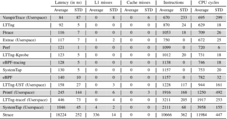
TABLE III: Average latency of a kernel space tracepoint Average (ns) STD 90th percentile None 17 0 17 LTTng 92 5 89 Ftrace 116 7 114 Perf 121 1 118 LTTng-Kprobe 123 5 121 eBPF-tracing 128 5 124 SystemTap 130 5 125 eBPF 140 10 126

In the graphs that follow, we show, for each run, the value of different metrics for each tracepoint call. By showing the results of all tracepoint calls for each tracer, it is much easier to find trends in the usage of different resources. Furthermore, this approach helps explaining corner cases, where a given set of circumstances influences the cost of a single tracepoint and helps setting an upper bound for the cost of an individual tracepoint, once the steady state is reached.

As explained in section VI-B, we sample performance counters at the beginning and end of each tracepoint invocation in order to precisely measure different metrics, such as the number of instructions executed, the number of cycles, or the number of cache misses. The number of instructions is directly related to the code logic and should not bring any surprise. Furthermore, although the number of instructions as an absolute value is not significant in isolation (compiler versions, options, etc. directly influence this value), it still is an interesting metric to capture, as it uncovers the different code paths that are taken by the program at runtime. Other metrics such as the number of cycles and the number of cache misses are interesting to show any erratic behavior. For instance, a larger number of cycles per instruction 5 (much

5_{This value depends on the architecture of the CPU. Superscalar processors}

can have multiple pipelines to achieve parallelism within a single processor. When that is the case, we can see a number of cycles per instructions that is lower than 1 (multiple instructions per cycle per processor). This paper focuses on multi-core scalar processors, which typically have one pipeline per processor.

higher than 1) might be due to contention over the memory bus, or to inefficient instructions. A lower number of cycles per instruction (closer to 1) could be a good sign, but it can often hint at potential optimizations, such as doing calculations in advance and caching them for future use. Added latency might be caused by an abnormally high number of page faults, and might help discover hard-to-detect and unexpected issues. On the other hand, these low-level metrics can confirm that everything is running smoothly, for instance, when most of the tracepoints seem to indicate a ratio of instructions per cycle close to 1.

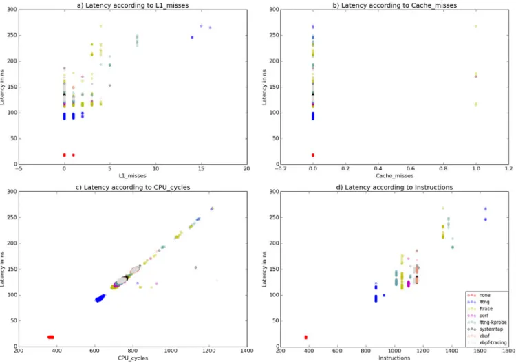
For all of the following graphs, the y-axis always shows the tracepoint latencies whereas the x-axis shows the values of different counters.

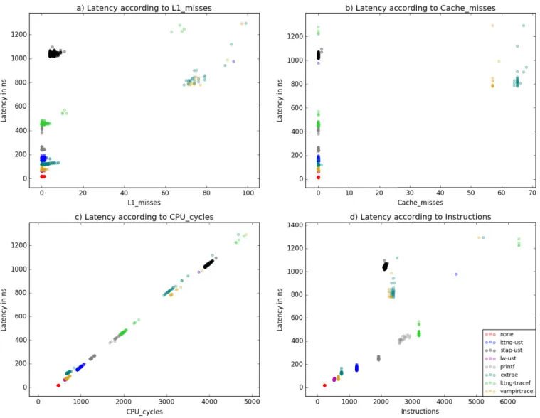
Looking at Figure 3 a) and b), it is interesting to note the lack of direct effect of the cache misses on the tracepoint latency. Contrary to what would have been expected, more L1 misses do not impact in any significant manner the cost of a tracepoint. We can make this assessment since the tracepoints that triggered 0 L1 misses range widely in the latency spectrum. Furthermore, tracepoints with higher L1 misses record similar latency as the ones with no misses. Of course, cache misses do affect latency, but their impact is diluted by other factors. We also notice that benchmarking in a steady state helps to keep the number of cache misses to a minimum, as shown in b).

On the other hand, CPU cycles have a direct linear relation with the latency of a tracepoint. However, this is more a consequence than a cause, since tracepoints are uninterruptible in our setup (interrupts disabled and the ones interrupted by NMIs are ignored) and the CPU frequency is maintained at a maximum, it is only natural that the more costly tracepoints require more CPU cycles. The interesting thing to note is that the nearly-perfect linear relation between CPU cycles and latency doesn’t exist with dynamic CPU frequency enabled. Since the CPU frequency can change dynamically, a high latency tracepoint can actually record a low number of cycles, changing the trend between latency and CPU cycles. A few outliers exist, potentially caused by an imprecision by sampling the pipeline to extract CPU cycles values

[Wilhelm, Grund, Reineke, Schlickling, Pister, and FerdinandWilhelm et al.2009]. Figure 3 d) shows a metric that directly impacts latency:

the number of instructions. As the number of instructions grows, the groups of samples are higher on the latency axis. As we might have expected, more instructions per tracepoint usually implies more time to complete and thus record a higher latency. With that said, the graph suggests that other factors impact the latency, as even for tracepoints that require the same number of instructions, their distribution on the latency spectrum is quite wide (tracepoints recorded using Ftrace that required 1052 instructions range between 110ns and 225ns).

Another interesting point that we can take from Figure 3 d) is the code path for each tracer. Looking at tracepoints sampled for LTTng, we can easily guess the three internal code paths of the tracer: the samples are grouped into three possible number of instructions: 870 instructions, 927 instructions, or 1638 instructions (for this particular build of LTTng and kernel). As explained in section V-A3, LTTng uses internal

sub-buffers with their size being a multiple of a page for its ring buffer. We might guess that these three code paths shown in the graph represent the tracepoints that cross boundaries: the tracepoints requiring 870 instructions to complete are the most frequent ones and execute the fast path. Storing the tracepoint into a sub-buffer is straightforward and translates to a simple memcpy(). The middle path, requiring 927 instructions, is covered when storing a tracepoint is still within the same sub-buffer but crosses page boundaries. The memory area backing a sub-buffer is manually managed by LTTng, and thus pages that make up a sub-buffer aren’t contiguous: LTTng doesn’t use virtual addresses but rather uses physical memory frames, which requires page stitching when data needs to be stored across (or read from) more than a single page. Finally, the slow path, requiring 1638 instructions, is covered by the tracepoints that cross sub-buffer boundaries (and implicitly page boundaries, as sub-buffers are page-aligned). LTTng then requires internal bookkeeping, such as writing some header data into the sub-buffer, which adds instructions to the critical path and further latency. Thus, if tracepoint latency is an issue, avoiding the slow path is possible by allocating larger sub-buffers and reducing the frequency of the slow path (although this might lead to other problems, such as events loss). With this information, it is possible to predict how many instructions an event might require, depending on the empty space left in the sub-buffer at the moment the tracepoint is hit. In other words, the middle and slow paths are taken at regular intervals. The middle path is taken every (PAGE_SIZE / EVENT_SIZE) events, and the slow path is taken every (SUB-BUFFER_SIZE / EVENT_SIZE)events, assuming all events are the same size.

This analysis can help the users choose the right buffer size to configure their tracer. In order to reduce the average tracepoint latency, the slow path should be avoided as much as possible. This is possible by setting larger sub-buffers. On the other hand, since sub-buffers can only be flushed once they are full, having larger sub-buffers usually implies a higher probability of event loss. Flushing large buffers requires more time, and if the events are recorded at a high rate, the ring buffer has time to loop and start overwriting unread sub-buffers before a single sub-buffer is consumed entirely. For a fixed buffer size, a trade-off has to be made between the number of sub-buffers and their size. Smaller sub-buffers reduce the risk of lost events, but larger sub-buffers result in faster tracepoints on average. We conclude this by mentioning that comparing the number of instructions per event between tracers isn’t necessarily a relevant metric, as the number of cycles an instruction requires may vary greatly and isn’t a direct indicator of latency (unless the numbers of instructions differ greatly). However, it is still interesting to analyze the number of instructions for the same tracer to deconstruct different code paths that have been taken, and get a deeper understanding of a tracer’s internals.

A similar observation can be made for Ftrace. However, we can only group the samples as executing one of two paths: 1052 instructions or 1341 instructions, which we reference respectively as the fast path and the slow path. The reason Ftrace samples only show two code paths, instead of 3 like

Fig. 3: All tracepoints latencies in kernel space against different hardware counters (Part 1)

LTTng, is the fact that Ftrace doesn’t use the notion of sub-buffers and only manipulates pages, albeit manually similarly to LTTng. Thus, a tracepoint recorded with Ftrace can only cover one of two cases: it either fits directly into a page, or it crosses page boundaries. This behavior can be achieved with LTTng if the size of the sub-buffers is set to the page size.

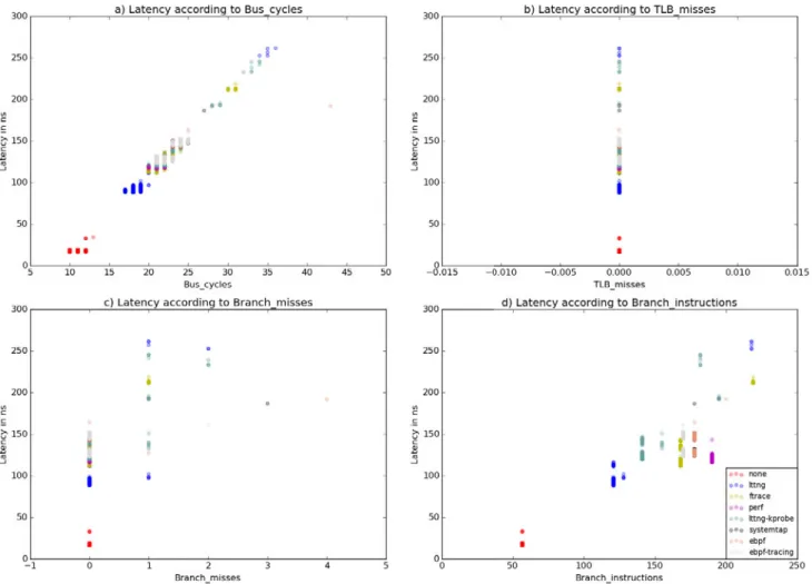
Figure 4 a), indicating the number of bus cycles per tracepoint, shows a result similar to Figure 3 c), which is naturally expected. Figure 4 b) shows that all tracepoints for all tracers are recorded without triggering any TLB misses. This is due to the fact that the events are sam-pled in the steady state and all TLB misses have already gradually been fulfilled. This is also to be expected as there are no outliers in the samples, since a TLB miss is costly relatively to the average tracepoint latency (memory accesses are orders of magnitude slower than cache accesses [Hennessy and PattersonHennessy and Patterson2011]).

Finally, Figure 4 c) showing the branch misses can support the theory about the slow and fast paths we discussed for Ftrace and LTTng. The binary is typically optimized for the fast path by the compiler (and by the pipeline at run-time), and thus should trigger no branch misses [SmithSmith1981]. Figure 4 c) validates this theory as most of the samples have 0 branch misses. When the tracepoint data to be written into

the ring buffer crosses a page boundary, a branch miss should occur when the remaining free size in the current page of the buffer is tested against the size of the event. This process explains sample where 1 branch miss happens. Looking at the raw data, we can confirm that all cases going through the slow (and middle) paths for Ftrace and LTTng trigger exactly 1 branch miss. The reciprocate of this hypothesis is also valid: all samples that trigger at least one branch miss are executing either the middle or slow path.

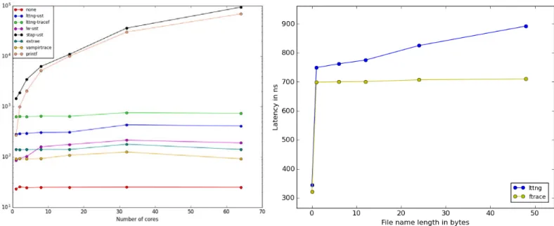
The difference in tracepoint latency between LTTng and LTTng-kprobe highlights the impact of the callback mecha-nism used by the tracer. We see that using Kprobes increases the frequency of L1 misses (Figure 3 a)) as well as the number of instructions per tracepoint (Figure 3 d)) which contribute to a higher overall latency. Table III shows that changing the callback mechanism from TRACE_EVENT to Kprobes adds around 30 ns of overhead.

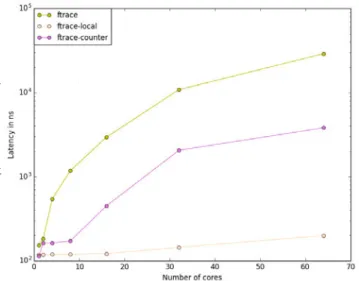
Figure 5 shows how the kernel tracers scale as the number of cores involved in the tracing effort grows. Notice that the la-tency axis is in logarithmic scale. Ftrace, eBPF and SystemTap show poor scalability, while LTTng and Perf scale with almost no added overhead. Such a significant performance impact on parallel systems usually indicates the use of an internal lock. It is indeed the case for Ftrace, as the global clock is protected

Fig. 4: All tracepoints latencies in kernel space against different hardware counters (Part 2)

Fig. 5: Average tracepoint latency in kernel space against the number of cores (Log scale)

using a spin lock [LoveLove2005]. When configured to use a global clock, Ftrace internally manages a data structure used as a clock source to timestamp all events. This data structure

simply holds the timestamp of the last clock value at the last timestamp, so that consecutive clock reads perceive the time as strictly monotonically increasing. However, as this clock is global to the system and shared amongst CPUs, proper synchronization is required to avoid concurrent writes. The following code, taken from the kernel source tree, shows a snippet of the global clock read function in Ftrace. In the following snippet, function sched_clock_cpu() reads the local CPU clock.

u64 notrace trace_clock_global(void) {

unsigned long flags; int this_cpu; u64 now; ... this_cpu = raw_smp_processor_id(); now = sched_clock_cpu(this_cpu); /*

* If in an NMI context then dont risk lockups * and return the cpu_clock() time:

*/