HAL Id: hal-01403951
https://hal.archives-ouvertes.fr/hal-01403951
Submitted on 28 Nov 2016HAL is a multi-disciplinary open access archive for the deposit and dissemination of sci-entific research documents, whether they are pub-lished or not. The documents may come from teaching and research institutions in France or abroad, or from public or private research centers.
L’archive ouverte pluridisciplinaire HAL, est destinée au dépôt et à la diffusion de documents scientifiques de niveau recherche, publiés ou non, émanant des établissements d’enseignement et de recherche français ou étrangers, des laboratoires publics ou privés.
Towards a unification of waterfalls, standard and P
algorithms
Serge Beucher
To cite this version:
Towards a unification of waterfalls, standard and P algorithms
Serge BeucherCenter of Mathematical Morphology, Mines ParisTech January 2012
1. Introduction
This paper can be considered as an addendum to the previous paper entitled "P algorithm, a dramatic enhancement of the waterfall transformation" [1]. In this former document, some suggestions have been made here and there, some ideas have emerged. These suggestions and ideas have unfortunately not be developped due to some lack of time and also because the authors did not wish to complicate the notions and concepts which were introduced.
The purpose of this present paper is to come back to these suggestions, to explore them in more details. We shall see that this exploration will lead to a generalisation of many segmentation transformations as watersheds, waterfalls, standard and P algorithms. This generalisation will give birth to a general segmentation procedure which unify the previously mentioned tools and which depends on two parameters only.
This paper aims also at describing an implementation of this general segmentation tool in the MAMBA library. It is a matter of fact that, since the publication of the P algorithm, a great number of requests have been forwarded to the authors regarding a usable implementation of this P algorithm. This MAMBA implementation brings an answer to these requests.
2. Notations
Let us recall the notations and operators which are used in this document.
2.1. Operators
- w is the valued watershed transform. The result is a function equal to 0 inside the catchment basins and to the altitude of the points belonging to the watershed lines.
- h is the hierarchical image generator. This operator can be applied to any image (positive function) f, but in this paper, it will be used mainly on segmentations (see below).
2.2. Images
- si denotes the final valued segmentation for the hierarchical level i.
- s'i+1 denotes the initial valued segmentation for the hierarchical level i. Generally, s'i ≠ si as the hierarchical process at level i aims at modifying this initial segmentation. s0 corresponds to the initial valued watershed (most of the time, it is a gradient watershed, but not always).
- h'i and hi are the hierarchical images corresponding respectively to s'i and si: h'i = h(s'i) ; hi = h(si)
- m is a numerical mask. It is an image made of two kinds of pixels: pixels at 0 or pixels with a value equal to the maximal possible value which can be defined depending on the depth of the image (for instance, with a 8-bit image, this value is 255). We often denote m as m(<condition>). When, at point x, <condition> is true, m takes its maximum value. When <condition> is false, m is equal to 0 at point x.
numerical images which are different from 0.
3. The various steps towards a unification
Remind that the algorithms described in [1] share the same general principle: reintroducing some of the contours which have been removed at each step of a waterfall transform (Fig. 1).
Fig. 1: Reminder of the three types of contours which are at stake in the waterfalls, standard and P algorithms. Type-1 contours should be always preserved, which is not the case in the classical waterfalls transformation.
3.1. An enhanced waterfalls transformation
Warning! In [1], standard and P algorithms were referenced as "enhanced waterfalls transformation". However, the enhanced waterfalls operator which is presented here is different. So, from now on, the expression "enhanced waterfalls" will designate only this operator.
Among the various types of contours which are analysed, it is a matter of fact that type-1 contours are always significant and should be kept. Indeed, standard and P algorithms both preserve these contours. However, it is not the case for the classical waterfalls transformation. Therefore, before entering more sophisticated procedures, it is easy to define an enhanced waterfalls transformation where type-1 contours are systematically preserved. In fact, this operator is defined as follows. If si is the current level of segmentation in the hierarchy, we can define its corresponding hierarchical image hi. Then, the valued watershed w of hi is realised. Finally, the corresponding hierarchical image hi+1 = h(w(hi)) is computed. The contours of si which are higher than or equal to hi+1 belong to the new segmentation level si+1.
This enhanced waterfalls transformation has some advantages. Firstly, it is not necessary to cope with possible biases occurring with the classical operator and which are described in [1, page 25]. Therefore, this algorithm is faster, easier to implement, especially when we look for the complete waterfalls hierarchy. It is, in particular, useless to calculate again the hierarchical image at each step. Indeed, the hierarchical image hi+1, although it has been calculated from the initial segmentation at level i+1 can be used at the next step as its minima contain all the minima, with a one-to-one correspondence, of the hierarchical image that would be built from the final segmentation si+1. So, at the next step, their respective watershed transforms are identical. Moreover, the resulting segmentation produced by this enhanced waterfalls transform is much better, as it is illustrated on some examples at Fig. 2.
the stopping criterion is the idempotence. When hi+1 is equal to 0, all the contours of si are reinjected and therefore si+1 = si.
Fig. 2: Examples of classical waterfalls transforms (middle images) and of enhanced waterfalls transforms (right images) calculated from the valued watersheds of the gradient of the original images (on the left). Only the last levels of hierarchy are given.
The reintroduction of type-1 contours dramatically enhances the final result. But this does not avoid the removal of some significant contours simply because they are lower than the final hierarchical image. These contours correspond to the maxima-islands introduced in [1] which appeared in the first levels of hierarchy and which were removed by the watershed transform (which, as a semi-homotopic operator, is not controlled by the maxima). This can be observed in the second example: the road marking (white dotted line) has disappeared because it corresponds to a maximum-island with a rather low height in the hierarchisation process.
3.2. A first generalisation of standard and P algorithms
Standard and P algorithms deal with the reintroduction of type-2 contours. Remind that these contours are defined as contours (belonging either to the previous segmentation or to the initial one) which are closer to the current hierarchical image than to 0.
Although it is claimed that sandard and P algorithms are non parametric transforms, the definition of type-2 contours leads, de facto, to the introduction of a parameter equal to 2, as it is discussed in [1, §8.2]. As suggested in this discussion, a first generalisation of these algorithms simply consists in replacing this hidden parameter by an explicit one, λ, called gain. Therefore, the definition of type-2 contours is modified accordingly. A type-2 contour is a contour Ck of the current segmentation si such that its initial altitude a0(Ck) fulfils the following inequality:
where hi+1 is the hierarchical image corresponding to the initial segmentation s'i+1. λ can be any real positive value.
In this extension, as it was already the case in the previous definition of P and standard algorithms, the relationship between s0 and hi+1 is a strict inequality:
λ s0>hi+1
If the gain λ is strictly greater than 1, this definition includes type-1 and type-2 contours. Indeed type-1 contours correspond to points of s0 such that λ s0≥hi+1(large inequality). Therefore, multiplying the altitude of these points by λ >1 insure that the strict inequality is fulfilled. However, when λ = 1, this definition does not correspond to the enhanced waterfalls transform described above. Indeed, some type-1 contours (those which are strictly equal to hi+1) are removed. This is very annoying since type-1 contours must always be preserved. To cope with this problem, one solution would be to replace the strict inequality by a large one:
λ s0≥hi+1
But this solution arises a new difficulty when λ is greater than 1. It tends to reinforce the influence of low contrasted contours in the first levels of hierarchy. For instance, when λ =2, contours at altitude 1 are preserved when they are surrounded by at least one contour at altitude 2. This gives to these contours a too important weight which induces negative effects on the following hierarchies and on the quality of the final result.
So, the function which hi+1 should be compared to is s0, ifs0≥hi+1orλ s0ifλ s0>hi+1.
In the digital case, these two conditions can be mixed by defining a composite function. We have: λ s0>hi+1→ λ s0≥hi+1+1 →(λ s0−1)≥hi+1
Therefore, the function used for the comparison is defined as (λ s0−1)∨s0and the condition which must be fulfilled to preserve contours is:
(λ s0−1)∨s0≥hi+1 This extension can be implemented in the following way:
• Compute (λ s0−1)∨s0(s0 is the initial valued watershed transform).
• From segmentation si (step i of the hierarchisation), compute its corresponding hierarchical image hi: hi = h(si).
• Compute the initial segmentation s'i+1: s'i+1 = w(hi).
• Compute the hierarchical image h'i+1 from s'i+1: h'i+1 = h(s'i+1). • Compute m ((λ s0−1)∨s0≥h 'i+1) .
• Remove the open (broken) contours in m and compute its corresponding binary mask M. • For standard algorithm, compute M '=M∩Siand the corresponding numerical mask m'. • For P algorithm, compute M '=M∩S0and the corresponding numerical mask m'. • The final segmentation si+1 is given by: si+1=m '∧(si∨hi+1)
As for the enhanced waterfalls transformation, the stopping criterion is the idempotence. This can be easily proved. If sN is the last non empty segmentation, we have s'N+1 = w(hN) = 0 and hN+1 = 0 (as hN contains a unique minimum). Therefore, M covers the entire space and sN+1 = sN.
The trick described above shows that it is possible to use a large range of comparison functions (as it was already suggested in [1], page 60). The general comparison inequality will then be, at each step:
ψ(s0)≥hi+1
where ψ is any function such that ψ≥I(extensive function). If ψ is not extensive, the result would be irrelevant.
ψ can also be any spatial function. This means that the comparison of each point of the contours to the current hierarchical image can be controlled not only by the height of the point but also by its
position in the image. This allows to introduce external information for a better control of this hierarchical segmentation. For instance, trends, illumination variations, regions of interest, textured regions could be taken into account. This extension offers a large scope of possibilities. Now, the real problem is to define correctly ψ in order that these features could be used.
Note that, although it may be indifferent to use hi+1 or h'i+1 in the standard segmentation (between h'i+1 and hi+1, no new minima appear), it is not true in practice. This is due to parity problems in the implementation of the watershed transform similar to those described in [1, page 63]. However, in P algorithm, using hi+1 is compulsory as new minima may be introduced at each level.
Note also that M∩S0and M are identical for P algorithm. The intersection is not necessary.
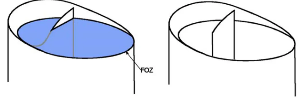
Fig. 3: When some points of a removed contour (FOZ lower than the hierachical image in blue) are higher than the hierarchical image (left), they must be suppressed otherwise they will be used for building the next hierarchical image which is likely to be erroneous (right).
You may also notice that a step of the implementation consists in removing broken contours in the mask function. These broken contours appear after the comparison as some points of these contours may be higher than h'i+1 although their lowest altitude is lower than the hierarchical image (Fig. 3). Thus, these contours are not completely removed. However, they must be suppressed otherwise the next hierarchical image would be erroneous. The fastest way to remove these contours is through a watershed transform of the mask function m. This is faster than a clipping procedure and, moreover, it is not depending of the complexity of the broken structures. Although it seems that this step is necessary only when working on valued watershed functions, in fact, it is not true. This procedure must be applied also on mosaic-gradient image. Indeed, if the points of the initial contours have the same height, it is not the case when we deal with higher levels of hierarchy since a single region may be surrounded by contours at different altitudes.
The last level of hierarchy of the CAR image in the standard segmentation is presented at Fig. 4 for three different values of the gain λ: 1.5, 2.0 and 3.0. The number of remaining contours increases as λ increases. This is obvious as, whatever the value of the gain, the number of hierarchy levels remains the same (4 in this example). Therefore the unique minimum in the last hierarchical image has always the same value. As the standard segmentation is nothing but a threshold of the previous remaining contours at an altitude proportional to 1/λ of the value of this minimum, this explains the result.
Fig.4: Results of the standard algorithm applied to the valued watershed of the gradient of image CAR (left) for different values of the gain λ (from left to right, 1.5, 2.0, 3.0).
Fig. 5: Using different values of the gain λ in P algorithm (from left to right: 1.5, 2.0 and 3.0).
In the same way, Fig. 5 illustrates some P algorithm results obtained with different values of λ (1.5, 2.0 and 3.0). Contrary to the standard segmentation, there is not necessarily an increasing of the remaining contours when λ increases. This is due to the fact that, contrary to the standard algorithm, new minima may appear in the successive hierarchical images. For the same reason, the number of hierarchical levels may vary as λ varies.
1.0 1.5 2.0 3.0
1
Level 4 Level 4 Level 4 Level 4
Level 6 Level 6 Level 6 Level 6
Level 7 Level 7 Level 7
Level 9 Level 9 2 3 4 5
3.3. A further extension
Introducing the gain λ allows to bridge the gap between the standard segmentation and the enhanced waterfalls transform. Another extension (which was also suggested in (1], page 44) brings the missing link between the standard and P algorithms. Indeed, the only difference between standard and P algorithms lies on the fact that, in standard algorithm, only contours belonging to the previous hierarchy are taken into account whereas, in P algorithm, all the contours (that is contours belonging to the first level of hierarchy - the initial watershed) are considered. When computing the (i+1)th level of hierarchy in standard algorithm, contours of Si are used, while contours of S0 are considered in P algorithm. So, it is possible to define a hierarchical segmentation where contours belonging to an intermediary level of hierarchy would be taken into account. This is achieved by introducing an offset k between the current level of hierarchy and the level which is used to select the contours to be compared to the current hierarchical image.
Implementing this extension consists in using simply Sj = Si-k instead of Si or S0 in the computation of the mask imageM '=M∩Sj. When k = 0, the standard segmentation is performed. When k = +∞ (sufficiently high in practice - 255 for a greyscale 8-bit image), P algorithm is realised.
Note that if (i - k) is negative, Sj (which does not exist) is replaced by S0. It is equivalent to define Sj as:
Sj=Smax(i− k ,0)
Note also that, when k > 0, some contours may oscillate in the successive hierarchies. However, due to the way the successive hierarchies are stored and coded (see below), this oscillation is most of the time masked and consequently has no effect on the hierarchies.
Fig. 6 shows the results (last levels of hierarchy) of this extended segmentation procedure applied to image TOOLS for different values of the gain λ and the offset k. When no image is given, this simply means that no change occurred since the previous segmentation obtained with a lower offset. Although it is difficult to bring into general from a single example, it seems nevertheless that the best results are obtained when the offset is maximum and for values of the gain around 2, which tends to validate the heuristic choice of these parameters made in [1].
4. Mamba implementations and performance
All the segmentation procedures described above have been implemented with the Mamba Image library. This open source library (X11 license), written in C and Python, is entirely devoted to mathematical morphology. It is freely available (version 1.0) with its documentation [2] at http://www.mamba-image.org. These new operators are not implemented in the current version (they will be in the next one). Therefore, the Python source code of these operators is given in annex, together with some add-ons which are needful to use them with the current version of Mamba.
The purpose of this implementation is twofold. Firstly, it answers some requests made to the author for an efficient and simple implementation of P algorithm. Unfortunately, until now, the available implementations of waterfalls and P algorithms use non open mathematical morphology software libraries. This implementation fills a gap. Secondly, it provides a strong basis for further experimentations with these tools, especially for tests on public image databases.
4.1. Description of the operators
Here is a brief description of the operators available in this Mamba implementation (see the annex for details).
- hierarchy generates the hierarchical image from the initial image (imIn) which can be a valued watershed or a mosaic-gradient or even a simple gradient. Image imMask (which is binary) contains the watershed lines of the initial image. The hierarchical image is put in imOut. The algorithm used to build the hierarchical image has been described in [3] and [1, page 20]. This operator is used by the other segmentation processes.
- hierarchicalLevel computes the next level of hierarchy from the current one, imIn (which is a valued watershed or a mosaic-gradient). From imIn, its hierarchical image is built, then the watershed transform is computed. Finally, a correction is applied (its description is given in [1, page 25]) in order to be sure that the next hierarchy is embedded in the previous one. This operator is only used by the classical waterfalls generator. It is useless for the other segmentation processes as the above mentioned correction is no more necessary.
- waterfalls is the classical waterfalls algorithm. From the initial image imIn (valued watershed or mosaic-gradient), it iterates the hierarchicalLevel operator to obtain the successive hierarchies of the waterfalls transformation in imOut. Each point in imOut takes the index value of the hierarchy where it appears for the last time (index 0 denotes the first level of hierarchy).
- enhancedWaterfalls implements the enhanced waterfalls transform where type-1 contours are always reintroduced. This implementation is faster than the waterfalls algorithm as the correction used in the previous approach (in hierarchicalLevel) is no longer necessary. Contours which are partly below the hierarchical image at each step are totally removed by means of a watershed transformation which acts as a skeleton by influence zones (SKIZ).
- standardSegment performs the standard segmentation with a gain λ as parameter (it is equal to 2 by default). The operator starts by computing the image equal to (λ s0−1)∨s0, where s0 is the initial valued watershed image in imIn. At each step, this image is compared to the current hierarchical image and contours which are above this hierarchical image and which were still present in the previous segmentation level are kept. The others are removed by a watershed transform.
- segmentByP computes P algorithm with a gain λ (2 by default). This algorithm is very similar to the previous one. The only difference (but it is of outmost importance) comes from the fact that all the initial contours are considered, not only those still present in the previous step of hierarchy. This small difference induces dramatic changes in the result of the segmentation.
- generalSegment mixes and extends the standard and P algorithms by introducing the offset k which allows to choose the hierarchy level used in the comparison with the current hierarchical image. More precisely, the offset indicates how far in the past we go to select the contours which will be compared.
generalSegment could be the only implemented operator. Indeed, if the offset is equal to 1, this
operator is identical to standardSegment. If offset is equal to 255, it is identical to segmentByP. Note also that the smallest value for the offset is 1 and not 0 in the software implementation (offset is defined from the hierarchical level to be built and not from the last already built one).
- extendedSegment is the last implemented operator. It can be considered as experimental. Contrary to the others, the function used in the comparison (namely (λ s0−1)∨s0) is not computed at the beginning of the process. Instead, a function ψ (see above) must be determined and entered in the operator. It corresponds to the imTest image. This extended segmentation should allow to take into account variations of luminance in the background, to reduce the influence of textured regions or
other features which may deteriorate the quality of the final segmentation.
All these operators store the successive hierarchies in the imOut image and they also return the number of hierarchy levels. Each level of hierarchy can be obtained by simply thresholding the imOut image.
4.2. Performances
These operators are built directly on the images. Although Mamba is fast, this could lead to slow operations compared to the performances which could be obtained by using approaches based on graphs [4]. However, these operators widely use the watershed transform and the geodesic reconstruction which are implemented in Mamba by means of hierarchical queues [5, 6]. These transformations are fast, so the computation speed of the hierarchical segmentation operators is not so bad as it is shown in the table below. These values have been obtained on 256x256 grey scale images with a dual core Intel processor running at 2.66 GHz on Windows XP. The average computation time per hierarchy level is less than 30 ms (Fig. 7). A better value could be obtained by using a more powerful processor and with a Linux operating system (mainly because it is a 64-bit OS). Preliminary tests indicate that a speed increase of about 50% can be expected.
Image Number ofhierarchies Computationtime (ms)
ROAD 4 110 ROUTE 4 110 CAR 5 141 TOOLS 7 219 BIRDS 7 187 PLANE 8 235 EAGLE 12 344
Fig. 7: Computation time for the generation of the successive hierarchical levels in P algorithm. The average time for computing one level is about 29 ms with the configuration described above.
On the other side, it is difficult to be sure that an implementation with graphs would be more efficient because this implementation needs to generate the graph from the image at the beginning of the process and to do the reverse operation at the end. Anyway, at this time, this graph implementation does not exist for P algorithm yet.
5. Conclusion and next steps
We have shown, through the introduction of two parameters, that various hierarchical segmentation algorithms belong to the same class of operators. By simply varying these two operators (gain λ and offset k), it is possible to sweep continuously a whole range of transformations, from the enhanced waterfalls transform (λ = 1, k = 0) to P algorithm (λ = 2, k = +∞) to standard segmentation (λ = 2, k = 0).
We have also provided a Mamba-based implementation of this class of transformations which is fast enough to allow the exploration of its efficiency, its properties and its characteristics. The first tests which have been realised reinforce the interest for P algorithm and for its parametric version. The introduction of the offset, although it seems promising, validates, at first, the choice of an infinite offset for potentially providing the best results for the segmentations. However, this path, together with the use of a general comparison image (extended segmentation) need to be further explored. Introducing parameters arises the problem of the choice of their optimal values in particular for the gain λ. Here again, a gain equal to 2.0 produces very often good results. However, it would be interesting to verify this point and, moreover, to find ways to automatically determine its best value. To this regard, the next step will consist in using image databases to test these operators and to try to assess their robustness. Instead of using the Berkeley database as it was the case in [1], database which provides a two important semantic content so that it is difficult to compare segmentations provided by human beings and by a low level algorithm, we intend to use a simpler database, the Segmentation Evaluation Database (available at http://www.wisdom.weizmann.ac.il/~vision/ Seg_Evaluation_DB/index.html) which seems more appropriate to test the efficiency of these segmentation algorithms.
6. References
[1] BEUCHER Serge and MARCOTEGUI Beatriz. P algorithm, a dramatic enhancement of the waterfall transformation. CMM/Mines Paristech publication, 86 pages. September 2009. (available at http://cmm.ensmp.fr/~beucher/publi/P-Algorithm_SB_BM.pdf)
[2] BEUCHER Nicolas. MAMBA documentation.(mambaApi Reference Manual).Web documents (available at http://www.mamba-image.org), 2009-2011.
[3] BEUCHER Serge. Watershed, hierarchical segmentation and waterfall algorithm. Proc. Mathematical Morphology and its Applications to Image Processing, Fontainebleau, Sept. 1994, Jean Serra and Pierre Soille (Eds.), Kluwer Ac. Publ., Nld, 1994, pp. 69-76.
[4] MARCOTEGUI Beatriz, BEUCHER Serge. Fast implementation of waterfall based on graphs. In Mathematical Morphology: 40 Years on : Proceedings of the 7th ISMM, Paris, April 18-20, 2005: Dordrecht: Springer, C. Ronse, L. Najman, and E. Decencière (eds.)p. 177-186.
[5] MEYER Fernand. Procédé de traitement d'images par files d'attente hiérarchisées. French Patent n° 91/033841, Institut National de la Propriété Industrielle, 20 mars 1991 (original document and its english translation can be found in the esp@cenet database).
[6] BEUCHER Nicolas and BEUCHER Serge. Hierarchical Queues: general description and imple-mentation in MAMBA Image library. Web publication available at http://cmm.ensmp.fr/ ~beucher/publi/HQ_algo_desc.pdf, April 2011.
This document is copyrighted under the Creative Commons "Attribution Non-Commercial No
Derivatives" license. For terms of use, see http://creativecommons.org/about/licenses/.
7. Annex
This annex contains the source scripts of the various operators described above. These scripts are somewhat redundant as the general structure of each operator is very similar. However, we preferred to keep this redundacy in order to clearly show the modifications which allow to extend these different operators.
To run these scripts, you will need to install Mamba, version 1.0. This software library is available at http://www.mamba-image.org. Read carefully the documentation before installation (Mamba requires other Python libraries, in particular the Python Imaging Library).
Important! These scripts require that you add in existing Mamba modules some operators which do not exist yet in version 1.0. You need in particular the multiplication of an image by a real constant value. This operator is available below. Just copy the Python script and add it at the end of the miscellaneous.py module:
def mulRealConst(imIn, v, imOut, nearest=False): """
Multiplies image imIn by a real positive constant value v and puts the result in image imOut. inIn and imOut can be 8-bit or 32-bit images. If imOut is a greyscale image (8-bit), the result is saturated (results of the multiplication greater than 255 are limited to this value). The constant v is truncated so that only its two first decimal digits are taken into account.
If 'nearest' is true, the result is rounded to the nearest integer value. If not (default), the result is simply truncated.
""" if imIn.getDepth()==1 or imOut.getDepth()==1: mamba.raiseExceptionOnError(mambaCore.ERR_BAD_DEPTH) imWrk1 = mamba.imageMb(imIn, 32) imWrk2 = mamba.imageMb(imIn, 1) v1 = int(v * 100) if imIn.getDepth()==8: imWrk1.reset()
mamba.copyBytePlane(imIn, 0, imWrk1) else: mamba.copy(imIn, imWrk1) mamba.mulConst(imWrk1, v1, imWrk1) if nearest: mamba.addConst(imWrk1, 50, imWrk1) mamba.divConst(imWrk1, 100, imWrk1) if imOut.getDepth()==8:
mamba.threshold(imWrk1, imWrk2, 255, mamba.computeMaxRange(imWrk1)[1]) mamba.copyBytePlane(imWrk1, 0, imOut)
imWrk2.convert(8)
mamba.logic(imOut, imWrk2, imOut, "sup") else:
mamba.copy(imWrk1, imOut)
Note also that, if you want to apply these operators on mosaic-gradient images, you will have to patch this transformation in the module segment.py. Indeed, this operator is faulty in Mamba, version 1.0. To apply the patch, simply copy the script below and replace the corresponding function in segment.py.
def mosaicGradient(imIn, imOut, grid=mamba.DEFAULT_GRID): """
Builds the mosaic-gradient image of 'imIn' and puts the result in 'imOut'. The mosaic-gradient image is built by computing the differences of two mosaic images generated from 'imIn', the first one having its watershed lines valued by the suprema of the adjacent catchment basins values, the second one been valued by the infima.
""" imWrk1 = mamba.imageMb(imIn) imWrk2 = mamba.imageMb(imIn) imWrk3 = mamba.imageMb(imIn) imWrk4 = mamba.imageMb(imIn) imWrk5 = mamba.imageMb(imIn) imWrk6 = mamba.imageMb(imIn, 1) mosaic(imIn, imWrk2, imWrk3, grid=grid) mamba.sub(imWrk2, imWrk3, imWrk1)
mamba.logic(imWrk2, imWrk3, imWrk2, "sup") mamba.negate(imWrk2, imWrk2)
mamba.threshold(imWrk3, imWrk6, 1, 255) mC.multiplePoints(imWrk6, imWrk6, grid=grid) mamba.convertByMask(imWrk6, imWrk3, 0, 255)
se = mC.structuringElement(mamba.getDirections(grid), grid) mC.dilate(imWrk1, imWrk4, se=se)
mC.dilate(imWrk2, imWrk5, se=se)
while mamba.computeVolume(imWrk3) != 0: mC.dilate(imWrk1, imWrk1, 2, se=se) mC.dilate(imWrk2, imWrk2, 2, se=se)
mamba.logic(imWrk1, imWrk3, imWrk1, "inf") mamba.logic(imWrk2, imWrk3, imWrk2, "inf") mamba.logic(imWrk1, imWrk4, imWrk4, "sup") mamba.logic(imWrk2, imWrk5, imWrk5, "sup") mC.erode(imWrk3, imWrk3, 2, se=se)
mamba.negate(imWrk5, imWrk5) mamba.sub(imWrk4, imWrk5, imOut)
Here is below the main script. Just copy it entirely and store it in a file named hierarchies.py. Then, you simply need to run this script to have all the hierarchical operators available in the Mamba Image library.
"""
This module provides a set of functions to perform hierarchical segmentations operations using mamba. it works with imageMb instance as defined in mamba. This module contains the waterfalls algorithm and various hierarchical
operators (enhanced waterfalls, standard hierarchy and P algorithm). """
# Contributor: Serge BEUCHER, Nicolas BEUCHER
import mamba
import mambaComposed as mC
def hierarchy(imIn, imMask, imOut, grid=mamba.DEFAULT_GRID): """
Construction of a hierarchical image from image 'imIn' and with 'imMask'. The binary image 'imMask' controls the dual reconstruction (propagation) of 'imIn'.
This operator is mainly used to build hierarchical images from valued watershed images.
The hierarchical image is put in 'imOut'. """ imWrk = mamba.imageMb(imIn) if mamba.checkEmptiness(imIn): mamba.copy(imIn, imOut) else: mamba.convertByMask(imMask, imWrk, 255, 0) mamba.logic(imIn, imWrk, imWrk, "sup") mamba.hierarDualBuild(imIn, imWrk) mamba.copy(imWrk, imOut)
def hierarchicalLevel(imIn, imOut, grid=mamba.DEFAULT_GRID): """
Computes the next hierarchical level of image 'imIn' in the waterfalls transformation and puts the result in 'imOut'.
This operation makes sure that the next hierarchical level is embedded in the previous one.
'imIn' must be a valued watershed image. """ imWrk0 = mamba.imageMb(imIn) imWrk1 = mamba.imageMb(imIn, 1) imWrk2 = mamba.imageMb(imIn, 1) imWrk3 = mamba.imageMb(imIn, 1) imWrk4 = mamba.imageMb(imIn, 32) mamba.threshold(imIn,imWrk1, 0, 0) mamba.negate(imWrk1, imWrk2)
hierarchy(imIn, imWrk2, imWrk0, grid=grid) mC.minima(imWrk0, imWrk2, grid=grid) mamba.label(imWrk2, imWrk4, grid=grid)
mamba.watershedSegment(imWrk0, imWrk4, grid=grid) mamba.copyBytePlane(imWrk4, 3, imWrk0)
mamba.threshold(imWrk0, imWrk2, 0, 0) mamba.diff(imWrk1, imWrk2, imWrk3) mC.build(imWrk1, imWrk3)
se = mC.structuringElement(mamba.getDirections(grid), grid) mC.dilate(imWrk3, imWrk1, 1, se)
mamba.diff(imWrk2, imWrk1, imWrk1)
mamba.logic(imWrk1, imWrk3, imWrk1, "sup") mamba.convertByMask(imWrk1, imWrk0, 255, 0) mamba.logic(imIn, imWrk0, imOut, "inf")
def waterfalls(imIn, imOut, grid=mamba.DEFAULT_GRID): """
Classical waterfall algorithm. All the hierarchical levels of greyscale image 'imIn' (which must be a valued watershed) are computed. 'imOut' contains all these hierarchies which are embedded, so that hierarchy i is simply obtained by a threshold in range [i+1, 255]. This transformation returns the number of hierarchical levels. """ imWrk1 = mamba.imageMb(imIn) imWrk2 = mamba.imageMb(imIn) imWrk3 = mamba.imageMb(imIn, 1) mamba.copy(imIn, imWrk1) imOut.reset() nbLevels = 0 mamba.threshold(imWrk1, imWrk3, 1, 255) while mamba.computeVolume(imWrk3) != 0: mamba.add(imOut, imWrk3, imOut)
hierarchicalLevel(imWrk1, imWrk2, grid=grid) mamba.threshold(imWrk2, imWrk3, 1, 255) mamba.copy(imWrk2, imWrk1)
nbLevels += 1 return nbLevels
def enhancedWaterfalls(imIn, imOut, grid=mamba.DEFAULT_GRID): """
Enhanced waterfall algorithm. Compared to the classical waterfalls
algorithm, this one adds the contours of the watershed transform which are above the hierarchical image associated to the next level of hierarchy. This waterfalls transform also ends to an empty set. All the hierarchical levels of image 'imIn' (which is a valued watershed) are computed. 'imOut' contains all these hierarchies which are embedded, so that hierarchy i is simply obtained by a threshold [i+1, 255] of image 'imOut'.
'imIn' and 'imOut' must be greyscale images. 'imIn' and 'imOu't must be different.
This transformation returns the number of hierarchical levels. """
imWrk2 = mamba.imageMb(imIn) imWrk3 = mamba.imageMb(imIn) imWrk4 = mamba.imageMb(imIn, 1) imWrk5 = mamba.imageMb(imIn, 32) mamba.copy(imIn, imWrk1) imOut.reset() nbLevels = 0 mamba.threshold(imWrk1, imWrk4, 1, 255) flag = not(mamba.checkEmptiness(imWrk4)) while flag:
mamba.add(imOut, imWrk4, imOut)
hierarchy(imWrk1, imWrk4, imWrk2, grid=grid) mC.valuedWatershed(imWrk2, imWrk3, grid=grid) mamba.threshold(imWrk3, imWrk4, 1, 255) flag = not(mamba.checkEmptiness(imWrk4)) hierarchy(imWrk3, imWrk4, imWrk2, grid=grid)
mamba.generateSupMask(imWrk2, imWrk1, imWrk4, strict=True) mamba.convertByMask(imWrk4, imWrk3, 255, 0)
mamba.logic(imWrk1, imWrk3, imWrk3, "inf") mamba.label(imWrk4, imWrk5, grid=grid)
mamba.watershedSegment(imWrk3, imWrk5, grid=grid) mamba.copyBytePlane(imWrk5, 3, imWrk1)
mamba.logic(imWrk1, imWrk3, imWrk1, "inf") mamba.threshold(imWrk1, imWrk4, 1, 255) nbLevels += 1
return nbLevels
def standardSegment(imIn, imOut, gain=2.0, grid=mamba.DEFAULT_GRID): """
General standard segmentation. This algorithm keeps the contours of the watershed transform which are above or equal to the hierarchical image associated to the next level of hierarchy when the altitude of the contour is multiplied by a 'gain' factor (default is 2.0). This transform also ends by idempotence. All the hierarchical levels of image 'imIn'(which is a
valued watershed) are computed. 'imOut' contains all these hierarchies which are embedded, so that hierarchy i is simply obtained by a threshold [i+1, 255] of image 'imOut'.
'imIn' and 'imOut' must be greyscale images. 'imIn' and 'imOut' must be different.
This transformation returns the number of hierarchical levels. """ imWrk0 = mamba.imageMb(imIn) imWrk1 = mamba.imageMb(imIn) imWrk2 = mamba.imageMb(imIn) imWrk3 = mamba.imageMb(imIn) imWrk4 = mamba.imageMb(imIn, 1) imWrk5 = mamba.imageMb(imIn, 1) imWrk6 = mamba.imageMb(imIn, 32) mamba.copy(imIn, imWrk1)
mC.mulRealConst(imIn, gain, imWrk6) mC.floorSubConst(imWrk6, 1, imWrk6)
mamba.threshold(imWrk6, imWrk4, 255, mamba.computeMaxRange(imWrk6)[1]) mamba.copyBytePlane(imWrk6, 0, imWrk0)
mamba.convert(imWrk4, imWrk2)
mamba.logic(imWrk0, imWrk2, imWrk0, "sup") mamba.logic(imWrk0, imWrk1, imWrk0, "sup") imOut.reset()
nbLevels = 0
mamba.threshold(imWrk1, imWrk4, 1, 255) flag = not(mamba.checkEmptiness(imWrk4)) while flag:
hierarchy(imWrk1, imWrk4, imWrk2, grid=grid) mamba.add(imOut, imWrk4, imOut)
mC.valuedWatershed(imWrk2, imWrk3, grid=grid) mamba.threshold(imWrk3, imWrk5, 1, 255) flag = not(mamba.checkEmptiness(imWrk5)) hierarchy(imWrk3, imWrk5, imWrk2, grid=grid)
mamba.generateSupMask(imWrk0, imWrk2, imWrk5, strict=False) mamba.logic(imWrk4, imWrk5, imWrk4, "inf")
mamba.convertByMask(imWrk4, imWrk3, 0, 255) mamba.logic(imWrk1, imWrk3, imWrk3, "inf") mamba.negate(imWrk4, imWrk4)
mamba.label(imWrk4, imWrk6, grid=grid)
mamba.watershedSegment(imWrk3, imWrk6, grid=grid) mamba.copyBytePlane(imWrk6, 3, imWrk3)
mamba.logic(imWrk1, imWrk2, imWrk1, "sup") mamba.logic(imWrk1, imWrk3, imWrk1, "inf") mamba.threshold(imWrk1, imWrk4, 1, 255) nbLevels += 1
return nbLevels
def segmentByP(imIn, imOut, gain=2.0, grid=mamba.DEFAULT_GRID): """
General segmentation by P algorithm. This algorithm keeps or reintroduces the contours of the initial watershed transform which are above or equal to the hierarchical image associated to the next level of hierarchy when the altitude of the contour is multiplied by a 'gain' factor (default is 2.0). This transform also ends by idempotence. All the hierarchical levels of image 'imIn' (which is a valued watershed) are computed. 'imOut' contains all these hierarchies which are embedded, so that hierarchy i is simply obtained by a threshold [i+1, 255] of image imOut.
'imIn' and 'imOut' must be greyscale images. 'imIn' and 'imOut' must be different.
This transformation returns the number of hierarchical levels. """ imWrk0 = mamba.imageMb(imIn) imWrk1 = mamba.imageMb(imIn) imWrk2 = mamba.imageMb(imIn) imWrk3 = mamba.imageMb(imIn) imWrk4 = mamba.imageMb(imIn, 1) imWrk5 = mamba.imageMb(imIn, 32) mamba.copy(imIn, imWrk1)
mC.mulRealConst(imIn, gain, imWrk5) mC.floorSubConst(imWrk5, 1, imWrk5)
mamba.threshold(imWrk5, imWrk4, 255, mamba.computeMaxRange(imWrk5)[1]) mamba.copyBytePlane(imWrk5, 0, imWrk0)
mamba.convert(imWrk4, imWrk2)
mamba.logic(imWrk0, imWrk2, imWrk0, "sup") mamba.logic(imWrk0, imWrk1, imWrk0, "sup") imOut.reset()
nbLevels = 0
mamba.threshold(imWrk1, imWrk4, 1, 255) flag = not(mamba.checkEmptiness(imWrk4)) while flag:
hierarchy(imWrk1, imWrk4, imWrk2, grid=grid) mamba.add(imOut, imWrk4, imOut)
mC.valuedWatershed(imWrk2, imWrk3, grid=grid) mamba.threshold(imWrk3, imWrk4, 1, 255) flag = not(mamba.checkEmptiness(imWrk4)) hierarchy(imWrk3, imWrk4, imWrk2, grid=grid)
mamba.generateSupMask(imWrk0, imWrk2, imWrk4, strict=False) mamba.convertByMask(imWrk4, imWrk3, 0, 255)
mamba.logic(imWrk1, imWrk3, imWrk3, "inf") mamba.negate(imWrk4, imWrk4)
mamba.label(imWrk4, imWrk5, grid=grid)
mamba.watershedSegment(imWrk3, imWrk5, grid=grid) mamba.copyBytePlane(imWrk5, 3, imWrk3)
mamba.logic(imWrk1, imWrk2, imWrk1, "sup") mamba.logic(imWrk1, imWrk3, imWrk1, "inf") mamba.threshold(imWrk1, imWrk4, 1, 255) nbLevels += 1
return nbLevels
def generalSegment(imIn, imOut, gain=2.0, offset=1, grid=mamba.DEFAULT_GRID): """
General segmentation algorithm. This algorithm is controlled by two parameters: the 'gain' (identical to the gain used in standard and P segmentation) and a new one, the 'offset'. The 'offset' indicates which level of hierarchy is compared to the current hierarchical image. The 'offset' is relative to the current hierarchical level. If 'offset' is equal to 1, this operator corresponds to the standard segmentation, if 'offset' is equal to 255 (this value stands for the infinity), the operator is equivalent to P algorithm.
Image 'imOut' contains all these hierarchies which are embedded. 'imIn' and 'imOut' must be greyscale images. 'imIn' and 'imOut' must be different.
This transformation returns the number of hierarchical levels. """ imWrk0 = mamba.imageMb(imIn) imWrk1 = mamba.imageMb(imIn) imWrk2 = mamba.imageMb(imIn) imWrk3 = mamba.imageMb(imIn) imWrk4 = mamba.imageMb(imIn, 1) imWrk5 = mamba.imageMb(imIn, 1) imWrk6 = mamba.imageMb(imIn, 32) mamba.copy(imIn, imWrk1)
mC.mulRealConst(imIn, gain, imWrk6) mC.floorSubConst(imWrk6, 1, imWrk6)
mamba.copyBytePlane(imWrk6, 0, imWrk0) mamba.convert(imWrk4, imWrk2)
mamba.logic(imWrk0, imWrk2, imWrk0, "sup") mamba.logic(imWrk0, imWrk1, imWrk0, "sup") imOut.reset() nbLevels = 0 mamba.threshold(imWrk1, imWrk4, 1, 255) flag = not(mamba.checkEmptiness(imWrk4)) while flag: nbLevels += 1
hierarchy(imWrk1, imWrk4, imWrk2, grid=grid) mamba.add(imOut, imWrk4, imOut)
v = max(nbLevels - offset, 0) + 1
mamba.threshold(imOut, imWrk4, v, 255)
mC.valuedWatershed(imWrk2, imWrk3, grid=grid) mamba.threshold(imWrk3, imWrk5, 1, 255) flag = not(mamba.checkEmptiness(imWrk5)) hierarchy(imWrk3, imWrk5, imWrk2, grid=grid)
mamba.generateSupMask(imWrk0, imWrk2, imWrk5, strict=False) mamba.logic(imWrk4, imWrk5, imWrk4, "inf")
mamba.convertByMask(imWrk4, imWrk3, 0, 255) mamba.logic(imWrk1, imWrk3, imWrk3, "inf") mamba.negate(imWrk4, imWrk4)
mamba.label(imWrk4, imWrk6, grid=grid)
mamba.watershedSegment(imWrk3, imWrk6, grid=grid) mamba.copyBytePlane(imWrk6, 3, imWrk3)
mamba.logic(imWrk1, imWrk2, imWrk1, "sup") mamba.logic(imWrk1, imWrk3, imWrk1, "inf") mamba.threshold(imWrk1, imWrk4, 1, 255) return nbLevels
def extendedSegment(imIn, imTest, imOut, offset=255, grid=mamba.DEFAULT_GRID): """
Extended (experimental) segmentation algorithm. This algorithm is controlled by image 'imTest'. The current hierarchical image is compared to image 'imTest'. This image must be a greyscale image. The 'offset' indicates which level of hierarchy is compared to the current hierarchical image.
The 'offset' is relative to the current hierarchical level (by default, 'offset' is equal to 255, so that the initial segmentation is used). Image 'imOut' contains all these hierarchies which are embedded. 'imIn', 'imTest' and 'imOut' must be greyscale images.
'imIn', 'imTest' and 'imOut' must be different.
This transformation returns the number of hierarchical levels. """ imWrk1 = mamba.imageMb(imIn) imWrk2 = mamba.imageMb(imIn) imWrk3 = mamba.imageMb(imIn) imWrk4 = mamba.imageMb(imIn, 1) imWrk5 = mamba.imageMb(imIn, 1) imWrk6 = mamba.imageMb(imIn, 32) mamba.copy(imIn, imWrk1) imOut.reset() nbLevels = 0
mamba.threshold(imWrk1, imWrk4, 1, 255) flag = not(mamba.checkEmptiness(imWrk4)) while flag:
nbLevels += 1
hierarchy(imWrk1, imWrk4, imWrk2, grid=grid) mamba.add(imOut, imWrk4, imOut)
v = max(nbLevels - offset, 0) + 1
mamba.threshold(imOut, imWrk4, v, 255)
mC.valuedWatershed(imWrk2, imWrk3, grid=grid) mamba.threshold(imWrk3, imWrk5, 1, 255) flag = not(mamba.checkEmptiness(imWrk5)) hierarchy(imWrk3, imWrk5, imWrk2, grid=grid)
mamba.generateSupMask(imTest, imWrk2, imWrk5, strict=False) mamba.logic(imWrk4, imWrk5, imWrk4, "inf")
mamba.convertByMask(imWrk4, imWrk3, 0, 255) mamba.logic(imWrk1, imWrk3, imWrk3, "inf") mamba.negate(imWrk4, imWrk4)
mamba.label(imWrk4, imWrk6, grid=grid)
mamba.watershedSegment(imWrk3, imWrk6, grid=grid) mamba.copyBytePlane(imWrk6, 3, imWrk3)
mamba.logic(imWrk1, imWrk2, imWrk1, "sup") mamba.logic(imWrk1, imWrk3, imWrk1, "inf") mamba.threshold(imWrk1, imWrk4, 1, 255) return nbLevels
This whole procedure will not be necessary with the next version (1.1) of Mamba which will contain these new operators.