HAL Id: hal-01309152
https://hal.archives-ouvertes.fr/hal-01309152
Submitted on 28 Apr 2016
HAL is a multi-disciplinary open access
archive for the deposit and dissemination of
sci-entific research documents, whether they are
pub-lished or not. The documents may come from
L’archive ouverte pluridisciplinaire HAL, est
destinée au dépôt et à la diffusion de documents
scientifiques de niveau recherche, publiés ou non,
émanant des établissements d’enseignement et de
Decomposing Cubic Graphs into Connected Subgraphs
of Size Three
Laurent Bulteau, Guillaume Fertin, Anthony Labarre, Romeo Rizzi, Irena
Rusu
To cite this version:
Laurent Bulteau, Guillaume Fertin, Anthony Labarre, Romeo Rizzi, Irena Rusu. Decomposing Cubic
Graphs into Connected Subgraphs of Size Three. The 22nd International Computing and
Combina-torics Conference (COCOON), Aug 2016, Ho Chi Minh City, Vietnam. �hal-01309152�
Decomposing Cubic Graphs into Connected
Subgraphs of Size Three
Laurent Bulteau1, Guillaume Fertin2, Anthony Labarre1, Romeo Rizzi3, and
Irena Rusu2
1 Universit´e Paris-Est, LIGM (UMR 8049), CNRS, ENPC, ESIEE Paris, UPEM, F-77454, Marne-la-Vall´ee, France
2 Laboratoire d’Informatique de Nantes-Atlantique, UMR CNRS 6241, Universit´e de Nantes, 2 rue de la Houssini`ere, 44322 Nantes Cedex 3, France
3 Department of Computer Science, University of Verona, Italy
Abstract. Let S = {K1,3, K3, P4} be the set of connected graphs of size 3. We study the problem of partitioning the edge set of a graph G into graphs taken from any non-empty S0⊆ S. The problem is known to be NP-complete for any possible choice of S0in general graphs. In this paper, we assume that the input graph is cubic, and study the computational complexity of the problem of partitioning its edge set for any choice of S0. We identify all polynomial and NP-complete problems in that setting, and give graph-theoretic characterisations of S0-decomposable cubic graphs in some cases.
1
Introduction
General context. Given a connected graph G and a set S of graphs, the S-decomposition problem asks whether G can be represented as an edge-disjoint union of subgraphs, each of which is isomorphic to a graph in S. The problem has a long history that can be traced back to Kirkman [7] and has been intensively studied ever since, both from pure mathematical and algorithmic point of views. One of the most notable results in the area is the proof by Dor and Tarsi [3] of the long-standing “Holyer conjecture” [6], which stated that the S-decomposition problem is NP-complete when S contains a single graph with at least three edges. Many variants of the S-decomposition problem have been studied while attempting to prove Holyer’s conjecture or to obtain polynomial-time algorithms in restricted cases [12], and applications arise in such diverse fields as traffic grooming [10] and graph drawing [5]. In particular, Dyer and Frieze [4] studied a variant where S is the set of connected graphs with k edges for some natural k, and proved the NP-completeness of the S-decomposition problem for any k ≥ 3, even under the assumption that the input graph is planar and bipartite (see Theorem 3.1 in [4]). They further claimed that the problem remains NP-complete under the additional constraint that all vertices of the input graph have degree either 2 or 3. Interestingly, if one looks at the special case where k = 3 and G is a bipartite cubic graph (i.e., each vertex has degree 3), then G can clearly be decomposed in polynomial time, using K1,3’s only, by selecting
either part of the bipartition and making each vertex in that set the center of a K1,3. This shows that focusing on the case k = 3 and on cubic graphs can lead
to tractable results — as opposed to general graphs, for which when k = 3, and for any non empty S0⊆ S, the S0
-decomposition problems all turn out to be NP-complete [4, 6].
In this paper, we study the S-decomposition problem on cubic graphs in the case k = 3 — i.e., S = {K1,3, K3, P4}. For any non-empty S0 ⊆ S, we settle
the computational complexity of the S0-decomposition problem by showing that the problem is NP-complete when S0 = {K1,3, P4} and S0 = S, while all
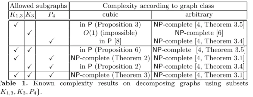
the other cases are in P. Table 1 summarises the state of knowledge regard-ing the complexity of decomposregard-ing cubic and arbitrary graphs usregard-ing connected subgraphs of size three, and puts our results into perspective.
Allowed subgraphs Complexity according to graph class K1,3 K3 P4 cubic arbitrary
X in P (Proposition 3) NP-complete [4, Theorem 3.5] X O(1) (impossible) NP-complete [6]
X in P [8] NP-complete [4, Theorem 3.4] X X in P (Proposition 6) NP-complete [4, Theorem 3.5] X X NP-complete (Theorem 2) NP-complete [4, Theorem 3.1] X X in P (Proposition 2) NP-complete [4, Theorem 3.4] X X X NP-complete (Theorem 3) NP-complete [4, Theorem 3.1] Table 1. Known complexity results on decomposing graphs using subsets of {K1,3, K3, P4}.
Terminology. We follow Brandst¨adt et al. [2] for notation and terminology. All graphs we consider are simple, connected and nontrivial (i.e. |V (G)| ≥ 2 and |E(G)| ≥ 1). Given a set S of graphs, a graph G admits an S-decomposition, or is S-decomposable, if E(G) can be partitioned into subgraphs, each of which is isomorphic to a graph in S. Throughout the paper, S denotes the set of connected graphs of size 3, i.e. S = {K3, K1,3, P4}. We study the following problem:
S0-decomposition
Input: a cubic graph G = (V, E), a non-empty set S0⊆ S. Question: does G admit a S0-decomposition?
We let G[U ] denote the subgraph of G induced by U ⊆ V (G). Given a graph G = (V, E), removing a subgraph H = (V0 ⊆ V, E0 ⊆ E) of G consists in
removing edges E0 from G as well as the possibly resulting isolated vertices. Finally, let G and G0 be two graphs. Then:
– subdividing an edge {u, v} ∈ E(G) consists in inserting a new vertex w into that edge, so that V (G) becomes V (G) ∪ {w} and E(G) is replaced with E(G) \ {u, v} ∪ {u, w} ∪ {w, v};
– attaching G0 to a vertex u ∈ V (G) means building a new graph H by iden-tifying u and some v ∈ V (G0);
– attaching G0 to an edge e ∈ E(G) consists in subdividing e using a new vertex w, then attaching G0 to w.
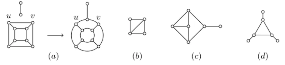
Figure 1 illustrates the process of attaching an edge to an edge of the cube graph, and shows other small graphs that we will occasionally use in this paper.
u v u v
(a) (b) (c) (d)
Fig. 1. (a) Attaching a new edge to {u, v}; (b) the diamond graph; (c) the co-fish graph; (d) the net graph.
2
Decompositions Without a K
1,3In this section, we study decompositions of cubic graphs that use only P4’s or
K3’s. Note that no cubic graph is {K3}-decomposable, since all its vertices have
odd degree. According to Bouchet and Fouquet [1], Kotzig [8] proved that a cubic graph admits a {P4}-decomposition iff it has a perfect matching. However, the
proof of the forward direction as presented in [1] is incomplete, as it requires the use of Proposition 1.(b) below, which is missing from their paper. Therefore, we provide the following proposition for completeness, together with another result which will also be useful for the case where S0= {K3, P4}.
Proposition 1. Let G be a cubic graph that admits a {K3, P4}-decomposition
D. Then, in D, (a) no K3 is used, and (b) no three P4’s are incident to the
same vertex.
Proof. Partition V (G) into three sets V1, V2 and V3, where V1 (resp. V2, V3) is
the set of vertices that are incident to exactly one P4 (resp. two, three P4’s) in
D. Note that V1is exactly the set of vertices involved in K3’s in D. Let ni= |Vi|,
1 ≤ i ≤ 3. Our goal is to show that n1= n3= 0, i.e. V1= V3= ∅. For this, note
that (1) each vertex in V3is the extremity of three different P4’s, (2) each vertex
in V2 is simultaneously the extremity of one P4 and an inner vertex of another
P4, while (3) each vertex in V1is the extremity of one P4. Since each P4 has two
extremities and two inner vertices, if p is the number of P4’s in D, we have:
• p = 3n3+n2+n1
2 (by (1), (2) and (3) above, counting extremities);
• p = n2
2 (by (2) above, counting inner vertices).
Putting together the above two equalities yields n1 = n3= 0, which completes
Since K3’s cannot be used in cubic graphs for {K3, P4}-decompositions by
Proposition 1 above, we directly obtain the following result, which implies that {K3, P4}-decomposition is in P.
Proposition 2. A cubic graph admits a {K3, P4}-decomposition iff it has a
perfect matching.
3
Decompositions Without a P
4In this section, we study decompositions of cubic graphs that use only K1,3’s or
K3’s.
Proposition 3. A cubic graph G admits a {K1,3}-decomposition iff it is
bipar-tite.
Proof. For the reverse direction, select either set of the bipartition, and make each vertex in that set the center of a K1,3. For the forward direction, let D be
a {K1,3}-decomposition of G, and let C and L be the sets of vertices containing,
respectively, all the centers and all the leaves of K1,3’s in D. We show that this
is a bipartition of V (G). First, C ∪ L = V since D covers all edges and therefore all vertices. Second, C ∩ L = ∅ since a vertex in C ∩ L would have degree at least 4. Finally, each edge in D connects the center of a K1,3 and a leaf of another
K1,3 in D, which belong respectively to C and L. Therefore, G is bipartite. ut
We now prove that {K1,3, K3}-decompositions can be computed in
poly-nomial time. Recall that a graph is H-free if it does not contain an induced subgraph isomorphic to a given graph H. Since bipartite graphs admit a {K1,3
}-decomposition (by Proposition 3), we can restrict our attention to non-bipartite graphs that contain K3’s (indeed, if they were K3-free, then only K1,3’s would be
allowed and Proposition 3 would imply that they admit no decomposition). Our strategy consists in iteratively removing subgraphs from G and adding them to an initially empty {K1,3, K3}-decomposition until G is empty, in which case we
have an actual decomposition, or no further removal operations are possible, in which case no decomposition exists. Our analysis relies on the following notion: a K3induced by vertices {u, v, w} in a graph G is isolated if V (G) contains no
vertex x such that {u, v, x}, {u, x, w} or {x, v, w} induces a K3.
Lemma 1. If a cubic graph G admits a {K1,3, K3}-decomposition D, then every
isolated K3 in G belongs to D.
Proof (contradiction). If an isolated K3 were not part of the decomposition,
then exactly one vertex of that K3 would be the center of a K1,3, leaving the
remaining edge uncovered and uncoverable. ut C6 is a minimal example of a cubic non-bipartite graph with K3’s that
ad-mits no {K1,3, K3}-decomposition: both K3’s in that graph must belong to the
Observation 1. Let G be a connected cubic graph. Then no sequence of at least one edge or vertex removal from G yields a cubic graph.
Proof (contradiction). If after applying at least one removal from G we obtain a cubic graph G0, then the graph that precedes G0 in this removal sequence must have had a vertex of degree at least four, since G is connected. ut Proposition 4. For any non-bipartite cubic graph G whose K3’s are all
iso-lated, one can decide in polynomial time whether G is {K1,3, K3}-decomposable.
Proof. We build a {K1,3, K3}-decomposition by iteratively removing K1,3’s and
K3’s from G, which we add as we go to an initially empty set D. By Lemma 1,
all isolated K3’s must belong to D, so we start by adding them all to D and
removing them from G; therefore, G admits a {K1,3, K3}-decomposition iff the
resulting subcubic graph G0 admits a {K1,3}-decomposition. Observe that G0
contains vertices of degree 1 and 2; we note that:
1. each vertex of degree 1 must be the leaf of some K1,3 in D;
2. each vertex of degree 2 must be the meeting point of two K1,3’s in D.
The only ambiguity arises for vertices of degree 3, which may either be the center of a K1,3 in D or the meeting point of three K1,3’s in D; however, there will
always exist at least one other vertex of degree 1 or 2 until the graph is empty (by Observation 1.). Therefore, we can safely remove K1,3’s from our graph and
add them to D by following the above rules in the stated order; if we succeed in deleting the whole graph in this way, then D is a {K1,3, K3}-decomposition of
G, otherwise no such decomposition exists. ut We conclude with the case where the graph may contain non-isolated K3’s.
Proposition 5. If a cubic graph G contains a diamond, then one can decide in polynomial time whether G is {K1,3, K3}-decomposable.
Proof. The only cubic graph on 4 vertices is K4, which is diamond-free and
{K1,3, K3}-decomposable, so we assume |V (G)| ≥ 6. Let D be a diamond in
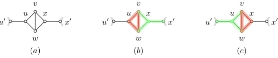
G induced by vertices {u, v, w, x} and such that {u, x} 6∈ E(G), as shown in Figure 2(a). D is connected to two other vertices u0 and x0 of G, which are respectively adjacent to u and x, and there are only two ways to use the edges of D in a {K1,3, K3}-decomposition, as shown in Figure 2(b) and (c). If u0= x0,
regardless of the decomposition we choose for D, u0and its neighbourhood induce a P3 in the graph obtained from G by removing the parts added to D. But
then that P3 cannot be covered, so no {K1,3, K3}-decomposition exists for G.
Therefore, we assume that u06= x0.
As Figure 2(b) and (c) show, either {u, v, w} or {v, w, x} must form a K3in
D, thereby forcing either {v, w, x, x0} or {u0, u, v, w} to form a K
1,3in D. In both
cases, removing the K3 and the K1,3 yields a graph G0 which contains vertices
of degree 1, 2 or 3. As in the proof of Proposition 4, Observation 1 allows us to make the following helpful observations:
1. every leaf in G0 must be the leaf of some K1,3 in D;
2. every vertex y of degree two in G0 must either belong to a K3 or be a leaf
of two distinct K1,3’s in D, which can be decided as follows:
(a) if y belongs to a K3 in G0, then it must also belong to a K3 in D;
otherwise, it would be the leaf of a K1,3 and the graph obtained by
removing that K1,3 would contain a P3, which we cannot cover;
(b) otherwise, y must be a leaf of two K1,3’s in D.
We therefore iteratively remove subgraphs from our graph and add them to D according to the above rules, which we follow in the stated order; if we succeed in deleting the whole graph in this way using either decomposition in Figure 2(b) or (c) as a starting point, then D is a {K1,3, K3}-decomposition of G, otherwise
no such decomposition exists. ut
v u w x u0 x0 v u w x u0 x0 v u w x u0 x0 (a) (b) (c)
Fig. 2. (a) A diamond in a cubic graph, and (b), (c) the only two ways to decompose it in a {K1,3, K3}-decomposition.
All the arguments developed in this section lead to the following result. Proposition 6. The {K1,3, K3}-decomposition problem on cubic graphs is
in P.
4
Decompositions That Use Both K
1,3’s and P
4’s
In this section, we show that problems {K1,3, P4}-decomposition and {K1,3,
K3, P4}-decomposition are NP-complete. Our hardness proof relies on two
intermediate problems that we define below and is structured as follows: cubic planar monotone 1-in-3 satisfiability
≤Pdegree-2,3 {K1,3, K3, P4}-decomposition with marked edges (Theorem 1 page 10)
≤P{K1,3, K3, P4}-decomposition with marked edges (Lemma 4 page 9)
≤P{K1,3, P4}-decomposition (Lemma 3 page 7)
We start by introducing the following intermediate problem: {K1,3, K3, P4}-decomposition with marked edges
Input: a cubic graph G = (V, E) and a subset M ⊆ E of edges.
Question: does G admit a {K1,3, K3, P4}-decomposition D such that no
edge in M is the middle edge of a P4 in D and such that every
The drawings that illustrate our proofs in this section show marked edges as dotted edges. The proof of Lemma 3 uses the following result.
Lemma 2. Let e be a bridge in a cubic graph G which admits a {K1,3, K3, P4
}-decomposition D. Then e must be the middle edge of a P4 in D.
Proof (contradiction). First note that e cannot belong to a K3 in D. Now
sup-pose e is part of a K1,3 in D. The situation is as shown below (without loss of
generality):
e
bank A bank B
If we remove from G the K1,3in D that contains e, then summing the terms of
the degree sequence of G[V (B)] yields 2 + 3(|V (B)| − 1) = 2|E(B)|, which means that 2|E(B)| ≡ 2 (mod 3), so |E(B)| 6≡ 0 (mod 3) and therefore B admits no decomposition into components of size three. The very same argument shows that if e belongs to a P4 in D, then it must be its middle edge, which completes
the proof. ut
Lemma 3. Let (G, M ) be an instance of {K1,3, K3, P4}-decomposition with
marked edges, and G0 be the graph obtained by attaching a co-fish to every edge in M . Then G can be decomposed iff G0admits a {K1,3, P4}-decomposition.
Proof. We prove each direction separately.
⇒: we show how to transform a decomposition D of (G, M ) into a decomposition D0 of G0. The subgraphs in D that have no edge in M are not modified. For the other subgraphs, we distinguish between four cases:
(a) if an edge of M belongs to a K1,3 in D, then attaching a co-fish does not
prevent us from adapting the decomposition of G in G0:
(b) if an edge of M belongs to a P4in D, then it is an extremity of that P4
and attaching a co-fish does not prevent us from adapting that part of the decomposition:
(d) if a K3in D has two edges in M , we can adapt the partition as follows:
⇐: we now show how to transform any {K1,3, P4}-decomposition D0of G0into a
decomposition of (G, M ). Again, the only parts of D0that will need adapting are those connected to the co-fishes that we inserted when transforming G into G0. Since the leaf u of the co-fish we inserted has a neighbour x such that {u, x} is a bridge in G0, {u, x} is the middle edge of a P
4 in D0 (Lemma 2)
and we may therefore assume without loss of generality that our starting point in G0 is as follows: u x v w G0: v w G :
with {v, w} 6∈ E(G0) since G is simple; therefore {u, w} cannot belong to a K3 in G0, and we have two cases to consider:
(a) if {u, w} belongs to a K1,3 in D0, that K1,3 can be mapped onto a K1,3
in D by replacing {u, w} with {v, w};
(b) otherwise, {u, w} is an extremal edge of a P4in D0; since {u, w} 6∈ E(G),
either that edge will remain in a P4 when removing the co-fish and
replacing {u, w} with {v, w}, or it will end up in a K3with either one or
two marked edges. Either way, the part can be added as such to D. ut We now show that we can restrict our attention to the following variant of {K1,3, K3, P4}-decomposition with marked edges. We say a graph is
degree-2,3 if its vertices have degree only 2 or 3.
degree-2,3 {K1,3, K3, P4}-decomposition with marked edges
Input: a degree-2,3 graph G = (V, E) and a subset M ⊆ E of edges. Question: does G admit a {K1,3, K3, P4}-decomposition D such that no
edge in M is the middle edge of a P4 in D and such that every
K3in D has either one or two edges in M ?
The following observation will help.
Observation 2. Let G be a degree-2,3 graph with |V2| degree-2 vertices. If G is
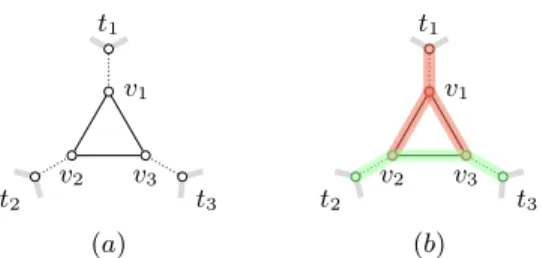
t1 t2 t3 v1 v2 v3 t1 t2 t3 v1 v2 v3 (a) (b)
Fig. 3. Adding a net (a) to a graph with degree-2 vertices t1, t2, t3(dotted edges belong to M0), and (b) its only possible decomposition (up to symmetry).
Proof. If G = (V, E) admits a {K1,3, K3, P4}-decomposition, then |E| ≡ 0
(mod 3). Let V2and V3 be the subsets of vertices of degree 2 and 3 in G. Then
2|V2| + 3|V3| = 2|E|, so 2|V2| ≡ 0 (mod 3). ut
We prove that allowing degree-2 vertices does not make the problem substantially more difficult, by adding the following gadgets until all vertices have degree 3. Let (G, M ) be an instance of degree-2,3 {K1,3, K3, P4}-decomposition with
marked edges, where G has at least three degree-2 vertices t1, t2, t3; by adding
a net over {t1, t2, t3}, we mean attaching a net by its leaves to v1, v2and v3and
adding the edges incident to the net’s leaves to M (see Figure 3(a)).
Proposition 7. Let (G, M ) be an instance of degree-2,3 {K1,3, K3, P4
}-de-composition with marked edges, where G has at least three degree-2 vertices t1, t2, t3, and let (G0, M0) be the instance obtained by adding a net to (G, M ).
Then (G0, M0) has three degree-2 vertices less than (G, M ), and (G, M ) can be
decomposed iff (G0, M0) can be decomposed.
Proof. By construction, G0 has fewer degree-2 vertices, since t1, t2, t3 now have
degree 3 instead of 2, other vertices of G are unchanged, and new vertices {v1, v2, v3} have degree 3. We now prove the equivalence.
⇒: given a decomposition D for (G, M ), we only need to add the K1,3 induced
by {v1, t1, v2, v3} and the P4 induced by {t2, v2, v3, t3} to cover the edges
of the added net in order to obtain a decomposition D0 for (G0, M0) (see Figure 3(b)).
⇐: we show that the only valid decompositions must include the choice we made in the proof of the forward direction. Indeed, the marked edges cannot be middle edges in a P4, and the K3induced by v1, v2and v3cannot appear as a
K3in a decomposition. Moreover, no marked edge can be the extremity of a
P4with two edges lying in the K3, since this would force another marked edge
to be the middle edge of a P4. Therefore the only possible decomposition of
the net is the one defined above (up to symmetry), and we can safely remove the P4 and the K1,3 from D0while preserving the rest of the decomposition.
u t Lemma 4. degree-2,3 {K1,3, K3, P4}-decomposition with marked edges
Proof. Given an instance (G, M ) of degree-2,3 {K1,3, K3, P4
}-decomposi-tion with marked edges, create an instance (G0, M0) by successively adding a net to any triple of degree-2 vertices, until no such triple remains. By Propo-sition 7, (G, M ) is decomposable iff (G0, M0) is decomposable. Moreover, either G0 is cubic (hence (G0, M0) is an instance of {K1,3, K3, P4}-decomposition
with marked edges), or G is trivially a no-instance by Observation 2. ut Finally, we show that degree-2,3 {K1,3, K3, P4}-decomposition with
marked edges is NP-complete. Our reduction relies on the cubic planar monotone 1-in-3 satisfiability problem [9]:
cubic planar monotone 1-in-3 satisfiability
Input: a Boolean formula φ = C1∧ C2∧ · · · ∧ Cn without negations over
a set Σ = {x1, x2, . . . , xm}, with exactly three distinct variables
per clause and where each literal appears in exactly three clauses; moreover, the graph with clauses and variables as vertices and edges joining clauses and the variables they contain is planar. Question: does there exist an assignment of truth values f : Σ → {true,
false} such that exactly one literal is true in every clause of φ? Theorem 1. degree-2,3 {K1,3, K3, P4}-decomposition with marked
ed-ges is NP-complete.
Proof. We first show how to transform an instance φ = C1 ∧ C2 ∧ · · · ∧ Cn
of cubic planar monotone 1-in-3 satisfiability into an instance (G, M ) of degree-2,3 {K1,3, K3, P4}-decomposition with marked edges. The
transformation proceeds by:
1. mapping each variable xionto a K1,3 denoted by K(xi) and whose edges all
belong to M ;
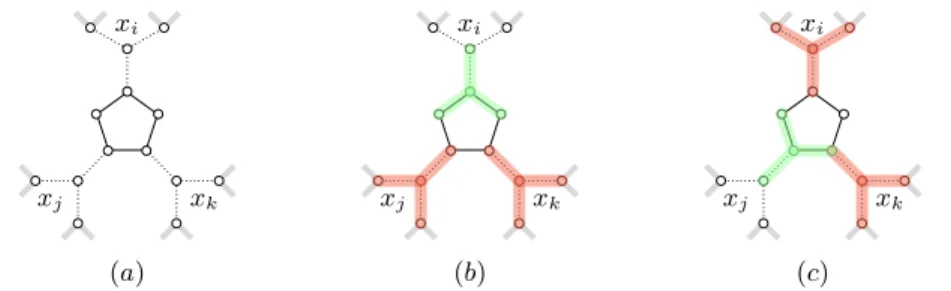
2. mapping each clause C = {xi, xj, xk} onto a cycle with five vertices in such
a way that K(xi), K(xj) and K(xk) each have a leaf that coincides with a
vertex of the cycle and exactly two such leaves are adjacent in the cycle. Figure 4 illustrates the construction, which yields a degree-2,3 graph. We now show that φ is satisfiable iff (G, M ) admits a decomposition.
⇒: we apply the following rules for transforming a satisfying assignment for φ into a decomposition D for (G, M ):
– if variable xi is set to false, then the corresponding K(xi) is added as
such to D;
– otherwise, the three edges of K(xi) will be the meeting points of three
different K1,3’s in the decomposition, one of which will have two edges
in the current clause gadget.
Two cases can be distinguished based on whether or not a leaf of K(xi) is
adjacent to a leaf of K(xj) or K(xk), but in both cases the rest of the clause
gadget yields a P4that we add as such to the decomposition (see Figure 4(b)
⇐: we now show how to convert a decomposition D for (G, M ) into a satisfying truth assignment for φ. First, we observe that D must satisfy the following crucial structural property:
For each clause C = (xi∨ xj∨ xk), exactly two subgraphs out of
K(xi), K(xj) and K(xk) appear as K1,3’s in D.
Indeed, G is K3-free by construction, and:
(a) if all of them appear as K1,3’s in D, then the remaining five edges of the
clause gadget cannot be decomposed;
(b) if only K(xi) appear as a K1,3 in D, then xj— without loss of generality
— must be a leaf either of a K1,3 in D with a center in the clause gadget
or of a P4in D with two edges in the clause gadget (the P4cannot connect
xj and xk, otherwise the rest of the gadget cannot be decomposed); in
both cases, the remaining three edges of the clause gadget must form a P4, thereby causing K(xk) to appear as a K1,3 in D, a contradiction (a
similar argument allows us to handle K(xj) and K(xk));
(c) finally, if none of them appear as K1,3’s in D, then xi must be the leaf
either of a K1,3 in D with a center in the clause gadget, or of a P4
with two edges in the clause gadget; in both cases, the remaining three edges of the clause gadget must form a P4 in D, which in turn makes it
impossible to decompose the rest of the graph.
Therefore, D yields a satisfying assignment for φ in the following simple way: if K(xi) appears as a K1,3in D, set it to false, otherwise set it to true. ut
Theorem 2. {K1,3, P4}-decomposition is NP-complete.
Proof. Immediate from Lemmas 3 and 4 and Theorem 1. ut
xi xj xk xi xj xk xi xj xk (a) (b) (c)
Fig. 4. (a) Connecting clause and variable gadgets in the proof of Theorem 1; dotted edges belong to M . (b), (c) Converting truth assignments into decompositions in the proof of Theorem 1; the only variable set to true is mapped onto a K1,3 in the decomposition; (b) shows the case where the only variable set to true — namely, xi — is such that K(xi) has no leaf adjacent to a leaf of K(xj) nor K(xk); (c) shows the other case, where xjis set to true and K(xi) and K(xk) have leaves made adjacent by the clause gadget.
A like-minded reduction1allows us to prove the hardness of {K
1,3, K3, P4
}-decomposition.
Theorem 3. {K1,3, K3, P4}-decomposition is NP-complete, even on K3-free
graphs.
5
Conclusions and Future Work
We provided in this paper a complete complexity landscape of {K1,3, K3, P4
}-decomposition for cubic graphs. A natural generalisation, already studied by other authors, is to study decompositions of k-regular graphs into connected components with k edges for k > 3. We would like to determine whether our positive results generalise in any way in that setting. It would also be interesting to identify tractable classes of graphs in the cases where those decomposition problems are hard, and to refine our characterisation of hard instances; for in-stance, does there exist a planarity-preserving reduction for Theorem 3? Finally, we note that some applications relax the size constraint by allowing the use of graphs with at most k edges in the decomposition [10]; we would like to know how that impacts the complexity of the problems we study in this paper.
References
[1] A. Bouchet and J.-L. Fouquet, Trois types de d´ecompositions d’un graphe en chaˆınes, in Combinatorial Mathematics: Proceedings of the In-ternational Colloquium on Graph Theory and Combinatorics, C. Berge, D. Bresson, P. Camion, J. F. Maurras, and F. Sterboul, eds., vol. 75 of North-Holland Mathematics Studies, North-Holland, 1983, pp. 131–141. [2] A. Brandst¨adt, V. B. Le, and J. P. Spinrad, Graph classes: a survey,
SIAM Monographs on Discrete Mathematics and Applications, Society for Industrial Mathematics, 1987.
[3] D. Dor and M. Tarsi, Graph decomposition is NP-complete: A complete proof of Holyer’s conjecture, SIAM J. Comput., 26 (1997), pp. 1166–1187. [4] M. E. Dyer and A. M. Frieze, On the complexity of partitioning graphs
into connected subgraphs, Discrete Appl. Math., 10 (1985), pp. 139–153. [5] ´E. Fusy, Transversal structures on triangulations: A combinatorial study
and straight-line drawings, Discrete Math., 309 (2009), pp. 1870–1894. [6] I. Holyer, The NP-completeness of some edge-partition problems, SIAM
J. Comput., 10 (1981), pp. 713–717.
[7] T. P. Kirkman, On a problem in combinatorics, Cambridge Dublin Math-ematical Journal, 2 (1847), pp. 191–204.
[8] A. Kotzig, Z teorie koneˇcn´ych pravideln´ych grafov tretieho a ˇstvrt´eho stupˇna, ˇCasopis pro pˇestov´an´ı matematiky, (1957), pp. 76–92.
[9] C. Moore and J. M. Robson, Hard tiling problems with simple tiles, Discrete Comput. Geom., 26 (2001), pp. 573–590.
1
[10] X. Mu˜noz, Z. Li, and I. Sau, Edge-partitioning regular graphs for ring traffic grooming with a priori placement of the ADMs, SIAM J. Discrete Math., 25 (2011), pp. 1490–1505.
[11] T. J. Schaefer, The complexity of satisfiability problems, in Proc. 10th STOC, San Diego, California, USA, May 1978, ACM, pp. 216–226. [12] R. Yuster, Combinatorial and computational aspects of graph packing and
A
Appendix: Omitted Proofs
Our hardness proof uses ideas similar to those used for {K1,3, P4
}-decomposi-tion, and is based on a slightly different intermediate problem. The structure is as follows:
monotone not-all-equal 3-satisfiability
≤P K3-free {K1,3, P4}-decomposition with marked edges (Theorem 4 page 14)
≤P {K1,3, K3, P4}-decomposition (Lemma 5 page 14)
We use the following intermediate problem.
K3-free {K1,3, P4}-decomposition with marked edges
Input: a cubic, K3-free graph G = (V, E) and a subset M ⊆ E of edges.
Question: does G admit a {K1,3, P4}-decomposition D such that no edge
in M is the middle edge of a P4 in D?
Lemma 5. Let (G, M ) be an instance of K3-free {K1,3, P4}-decomposition
with marked edges, and G0 be the graph obtained by attaching a co-fish to every edge in M . Then G can be decomposed iff G0 admits a {K1,3, K3, P4
}-de-composition.
Proof. The proof of the forward direction is exactly the same as that of the forward direction of Lemma 3. For the reverse direction, let D0 be a {K1,3,
K3, P4}-decomposition of G0. The only K3’s in G0 are those that belong to the
co-fishes we inserted, so we only need to show that removing those co-fishes does not prevent us from adapting the decomposition of G0 in order to obtain a {K1,3, P4}-decomposition D of G. The proof is similar to that of the reverse
direction of Lemma 3, with the following modification: since G is K3-free, we
have NG(u) ∩ NG(w) = ∅, so if {u, w} is the extremal edge of a P4 in D0, then
it will map onto {v, w} in G, where it will become the extremal edge of a P4in
D (as opposed to, possibly, a K3in the proof of Lemma 3). ut
We give a reduction from the following NP-complete variant of sat [11]: monotone not-all-equal 3-satisfiability
Input: a Boolean formula φ = C1∧ C2∧ · · · ∧ Cn without negations over
a set Σ = {x1, x2, . . . , xm}, with exactly three distinct variables
per clause.
Question: does there exist an assignment of truth values f : Σ → {true, false} such that exactly one or two literals are true in every clause of φ?
Theorem 4. K3-free {K1,3, P4}-decomposition with marked edges is
Proof. Given an instance φ of monotone not-all-equal 3-satisfiability, we build an instance (G, M ) of K3-free {K1,3, P4}-decomposition with
marked edges as follows:
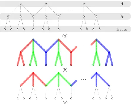
1. For each variable xi with k occurrences (we can assume k ≥ 2), we create a
tree T (xi) with 3k leaves, called a variable tree, whose edges are all marked
(see Figure 5(a)). Edges incident to a leaf are called border edges, the others are called internal edges.
2. For each clause xi∨ xj∨ xk, we create a P7 (v1, v2, . . . , v7), called a clause
path, with marked edges {v2, v3} and {v5, v6}, to which we join three border
edges of each variable tree as follows (see Figure 6):
• one leaf of T (x1) is joined to v1, another to v3, and another to v7;
• one leaf of T (x2) is joined to v1, another to v5, and another to v7;
• one leaf of T (x2) is joined to v2, another to v4, and another to v6.
Note that the resulting graph is indeed cubic: each inner vertex of a variable tree has degree 3, and each leaf is also part of a clause path. Furthermore, the inner vertices of a clause path are adjacent to two other vertices in the path and one other vertex in a variable tree, and each endpoint of a clause path is adjacent to another vertex in the path and two vertices in different variable trees.
We further observe that G is K3-free. First, any cycle included only in variable
trees has length at least 4 (since it must be included in at least 2 such tree, and in each tree the path between any pair of leaves has length at least 2). Therefore, a K3 would have to use 1 or 2 edges in a clause path. If it uses only one edge
{vi, vi+1}, then both vi and vi+1 must be joined to leaves of the same variable
tree, which is impossible since each clause consists of three different variables. If two edges are used, then the last edge of the K3 would be joining two leaves in
some variable tree, which is also impossible. Therefore, G is K3-free.
We now prove that φ is satisfiable iff (G, M ) admits a decomposition. ⇒: From a satisfying truth assignment, we create a {K1,3, P4}-decomposition
of (G, M ) as described in Figures 5(b − c) and 6(b − e). Specifically, for each variable xiwith k occurrences, if xi= true, then we cover all edges of T (xi)
with 2k − 1 K1,3’s (Figure 5(b)). If xi = false, then we cover all internal
edges of T (xi) with k − 1 K1,3’s(Figure 5(c)).
Now for any clause xi∨ xj∨ xk, at least 1 and at most 2 variables among
{xi, xj, xk} are set to false. For these two variables and the corresponding
variable trees, the border edges are still uncovered (for variables assigned true, border edges are covered with the rest of the variable tree). Each tree has 3 border edges coming to the clause path, so there are either 9 or 12 edges to cover (6 in the clause path and 3 or 6 in border variable trees). As shown in Figures 5(b − e), there always exist a decomposition of these edges into K1,3’s and P4’s (with the constraint that no marked edge is the middle
of a P4).
Overall, all edges in all variable trees and clause paths are covered by a K1,3
A B leaves . . . (a) . . . (b) . . . (c)
Fig. 5. (a) A variable tree T (xi) for a variable xiwith k occurrences: all its edges are marked, and it has 3k leaves. Internal vertices are partitioned into two sets A and B. (b) A decomposition of T (xi), corresponding to xi= true. (c) A decomposition of the internal edges of T (xi), corresponding to xi= false.
⇐: We first consider any variable tree, and show that the decompositions used for true and false assignments above are in fact the only two possible decompositions of the internal edges of this tree. Indeed, consider internal vertices and their partition into A and B (see Figure 5(a)): because of marked edges, all edges between any two internal vertices must be part of a K1,3,
linking a leaf to a center. Since internal vertices form a path, they must alternate along this path between leaves and centers of K1,3’s, so either all
vertices of B are centers, or all vertices of A are centers. Each case yields only one possible decomposition of adjacent edges, as described respectively in Figures 5(b) and 5(c). Naturally, we assign true to any variable whose tree is decomposed as in the first case, and false to other variables. We further make the following observation for the false case: consider any leaf x of the tree, and its parent y. Due to marked edges, x can only be the center of a K1,3, or a middle node of a P4, of which y is an endpoint.
We now consider a clause xi∨xj∨xk, and show that its variables can neither
be all set to true nor all set to false. Aiming at a contradiction, assume first that all variables are set to true. Then all border edges of their trees are already covered, and the K1,3’s and P4’s covering the clause path may
only use the 6 edges of the path. The only possibility to decompose the path in such a way is to use two P4’s, however, such P4’s would have marked
v1 v2 v3 v4 v5 v6 v7 T (xi) T (xj) T (xk) (a) v1 v2 v3 v4 v5 v6 v7 T (xi) T (xj) T (xk) T (xi) T (xj) T (xk) v1 v2 v3 v4 v5 v6 v7 T (xi) T (xj) T (xk) T (xi) T (xj) T (xk)
(b) xi= true, xj= true, xk= false (c) xi= true, xj= false, xk= true
v1 v2 v3 v4 v5 v6 v7 T (xi) T (xj) T (xk) T (xi) T (xj) T (xk) v1 v2 v3 v4 v5 v6 v7 T (xi) T (xj) T (xk) T (xi) T (xj) T (xk)
(d) xi= false, xj= true, xk= false (e) xi= false, xj= false, xk= true Fig. 6. (a) A clause path and its connections to the variable trees. (b − e) For each truth assignment of xi, xj, xk (up to symmetry), a decomposition of the path edges
edges as middle edges, which is forbidden. We now assume that all variables of a clause are set to false, i.e. it remains to cover the clause path and all border edges of the variable trees. Thanks to the observation made on leaves of the tree in the false case, vertices v1and v2are either centers of K1,3’s,
or middle nodes in P4’s. They cannot both be centers of K1,3’s, and due to
marked edges, they must both be middle nodes of the same P4. However,
as noted above, the parents of v1 in both trees T (xi) and T (xj) should be
endpoints of this P4, which is impossible.
Finally, each variable has been assigned a truth value, and for each clause there must be at least one true and one false variable: therefore, we have a satisfying assignment for our instance of monotone not-all-equal 3-satisfiability.
u t